Identifying soil compressibility from pressuremeter test

HAL Id: hal-01008284

https://hal.archives-ouvertes.fr/hal-01008284

Submitted on 29 Apr 2018

HAL is a multi-disciplinary open access

archive for the deposit and dissemination of sci-entific research documents, whether they are pub-lished or not. The documents may come from teaching and research institutions in France or abroad, or from public or private research centers.

L’archive ouverte pluridisciplinaire HAL, est destinée au dépôt et à la diffusion de documents scientifiques de niveau recherche, publiés ou non, émanant des établissements d’enseignement et de recherche français ou étrangers, des laboratoires publics ou privés.

Identifying soil compressibility from pressuremeter test

Damien Rangeard, Christophe Dano, Philippe Marchina

To cite this version:

Damien Rangeard, Christophe Dano, Philippe Marchina. Identifying soil compressibility from pres-suremeter test. International Symposium on Numerical Models in Geomechanics (NUMOG IX), 2004, Ottawa, Canada. �hal-01008284�

1 INTRODUCTION

Since soils are usually remoulded by sampling, the mechanical properties determined in the laboratory are questionable. Therefore, soil characterization by inverse analysis of in situ tests has become an attractive method to identify soil parameters in geotechnical engineering. However, a parameter of a constitutive model can be reliably identified by inverse analysis only if this parameter has a significant effect on the stress – strain or load – displacement curve deduced from the experience. For instance, the value of the Poisson’s ratio has a negligible effect on the pressuremeter curve (relation between the pressure and the displacement at the cavity wall) because of the almost purely deviatoric stress path.

Likewise, assuming the Modified Cam-Clay model, the quantity β = λ - κ where λ and κ are respectively the slope of the virgin consolidation and of the swelling line in the (e- ln p’) diagram, has no effect on the pressuremeter curve in clayed soils (β > 0.2), both in drained and undrained conditions (Rangeard et al. 2003). The matter of this paper is to discuss about the effect of β when β is lower than 0.2 (such a value is typical of sandy soils) and to investigate the possibility to simultaneously identify several constitutive parameters.

2 PRESSUREMETER TEST MODELISATION

2.1 Geometry and boundary conditions

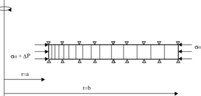
Numerical simulations of pressuremeter tests are performed using the finite elements code Cesar-LCPC. Axisymetric geometry and plane strain conditions, following the recommendations by Houlsby & Carter (1993) when the height to diameter ratio of the pressuremeter probe is greater than 6, are assumed (Fig. 1).

As previously indicated by Bahar (1992), the condition of infinite medium is obtained for a ratio of the outer diameter (2b) to the inner diameter (2a) equal to 50, whereas a value of 30 is enough for clay materials (Zentar et al. 1998).

σr0 + ∆P

σr0

r=a

r=b

Figure 1. FEM model.

2.2 Constitutive model and initial state of soil

The Modified Cam-Clay model (Roscoe & Burland 1968) with an isotropic and linear elasticity is

Identifying soil compressibility from pressuremeter test

D. Rangeard

Laboratoire de Génie Civil et Génie Mécanique, Institut National des Sciences Appliquées, Rennes, France

C. Dano

Research Institute in Civil and Mechanic Engineering, Ecole Centrale Nantes – University of Nantes - CNRS, France

P. Marchina

Total Company, Pau, France

ABSTRACT: Inverse analysis of pressuremeter tests has been widely used to identify the parameters of low

permeability soils assuming the modified Cam-Clay model. In such a case, the simultaneous identification of two parameters (for instance, the consolidation pressure pc0 and the critical state parameter M) can be

achieved from a single pressuremeter curve obtained in fully drained conditions. Additional experimental information is therefore required to determine the others parameters of the constitutive model. This paper focuses especially on the determination of the plastic compressibility β (where β=λ−κ) of prime importance in many engineering problems. Based on sensitivity studies, a procedure to identify simultaneously the plastic compressibility and the parameters M and p’c0 is proposed.

assumed to represent the behavior of the soil. In subsequent numerical simulations, the soil is fully saturated and the permeability is isotropic.

A reference set of Modified Cam-Clay parameters and an initial state of stress is presented in Table 1. In Table 1, G is the shear modulus of the soil, M the slope of the critical state line in the (q – p’) plane, e the void ratio and p’c0 the preconsolidation pressure.

σ’r0, σ’v0 and u0 are respectively the initial radial

effective stress, the initial vertical effective stress and the initial pore pressure. u0 is set to 0, so that

computations directly provide the value of the pore pressure variation ∆u. The initial state of stress corresponds to an isotropic overconsolidation ratio value of 1 and a coefficient of earth pressure at rest K0 equal to 0.5.

Table 1. Modified Cam-Clay parameters.

__________________________________________________ G β M p’c0 σ’r0 σ’v0 u0 __________________________________________________ MPa kPa kPa kPa kPa __________________________________________________ 30.8 0.06 1.2 280 150 300 0 __________________________________________________

2.3 Drainage conditions

Due to the non homogeneous stress field generated around the cavity, a partial drainage can occur during the pressuremeter test. The partial drainage depends on the loading rate and/or the permeability of the soil. It also induces changes in the soil characteristics. The drainage condition is consequently of great importance in order to accurately interpret a pressuremeter test. Rangeard et al. (2002) showed that the drainage condition depends on a dimensionless coefficient Dk expressed

as : k a t Dk a0 ∂ ε ∂ = (1)

This coefficient depends on the radial permeability k, the initial radius of the cavity a (a = 50 mm) and the initial strain rate of the test ∂εa0/∂t.

Rangeard et al. (2002) have shown that four kinds of drainage conditions can be defined following the values of the radial permeability and the initial strain rate of the test. The fully drained conditions are obtained for high permeability and low strain rate: the value of Dk has to be lower than 10-2. The fully

undrained conditions are obtained for low permeability and high strain rate: the value of Dk has

to be greater than 102. The partially drained type A behavior is characterized by an effect of the drainage on both the total stresses and the pore pressure. The partially drained type B behavior is an “undrained” behavior regarding the total stresses whereas the pore pressure is not completely developed.

The previous observation also means that a constant value of the ratio k/(∆P/∆t), where P is the pressure at the cavity wall, leads to the same

pressuremeter curve. Therefore, the stress rate ∆P/∆t is subsequently kept constant (∆P/∆t = 20 kPa/min) and the different drainage conditions are simulated by changing the value of the soil permeability k. For a shear modulus G of 30.8 MPa (Tab. 1), the initial strain rate defined as:

G 2 t / P 0 a = ∆ ∆ ε• (2)

is equal to 5.4x10-6 s-1. The fully undrained conditions are then achieved for a value of the permeability k lower than 2.7x10-9 m/s whereas the fully drained conditions are obtained for a permeability greater than 3x10-5 m/s.

Computations are performed assuming the following values of k: k = 10-10 m/s for the fully undrained conditions and k = 10-1 m/s for the fully drained conditions.

2.4 Compressibility effect

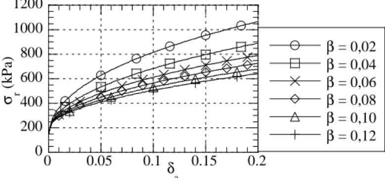
Figure 2 represents the effect of the plastic compressibility β on the pressuremeter curve when β is between 0.02 and 0.12 (corresponding Cc values

are 0.05 and 0.25). The values of the other parameters are reported in Table 1. In Figure 2, δa is

the ratio of the displacement of the cavity wall to the initial radius a of the cavity and σr = σr0 + ∆P is the

radial stress at the cavity wall.

As previously indicated, β has no effect on the pressuremeter curve for values greater than 0.2. This is no longer the case when the value of β is typical of sandy formation in fully drained conditions, namely for values between 0.02 and 0.12 (Fig. 2). β has therefore to be considered as a key factor for the inverse procedure. 0 200 400 600 800 1000 1200 0 0.05 0.1 0.15 0.2 β = 0,02 β = 0,04 β = 0,06 β = 0,08 β = 0,10 β = 0,12 σ r ( k P a) δ_a

Figure 2. β effect on the pressuremeter curve in fully drained conditions.

3 PARAMETERS IDENTIFICATION 3.1 Inverse analysis procedure

The classical resolution of a mechanical problem consists of calculating the response “R” of a mechanical system “S” subjected to actions “C”. The system «S» includes the constitutive model “M” and

its parameters “P”. Such a problem, known as a direct problem, can be mathematically expressed by:

( )

R= (3)

where F represents functional calculus connecting “R” (to be determined) to S (known).

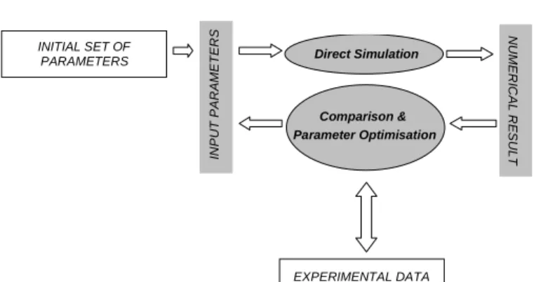
When an in situ test is performed, the parameters “P” of the chosen constitutive model “M” are unknown. However, the experimental response “R*” provides complementary information in order to rebuild the unknown soil characteristics by inverse analysis (Fig. 3). More precisely, the set of parameters “P” of the constitutive model “M” can be determined by iterative computations which gradually minimize the difference between the experimental data and the computational outcomes (Fig. 4). Formally, the difference between the observation data and the model prediction is formulated as:

∫

where the notation represents a norm in the space variable, t1-t0 is the time of observation, and R*

(t)-R(S,t) is the difference between experimental and numerical data.

In practice, the observable quantities (displacements, forces, …) were collected at discrete moments. Therefore, Equation 4 can be transformed as a discrete sum where Mn is the number of

measurements and (D) is a weighting matrix (Eq. 5).

[

]

∑

Figure 3. Definition of the inverse problem.

EXPERIMENTAL DATA INITIAL SET OF

PARAMETERS Direct Simulation

Comparison & Parameter Optimisation N U ME R IC A L R E S U L T IN P U T P A R A ME T E R S

Figure 4. Identification process.

The matrix D allows to transform the observable variables into dimensionless ones by dividing each of them by the square of the inverse of the error estimation, within the measure of each variable (Pilvin and Cailletaud, 1994).

Two codes, the finite elements code Cesar-LCPC and the optimization code SiDoLo, are coupled through an interface program called InCeSi as indicated in Figure 4 (Zentar et al. 2001). The inverse analysis procedure is the following:

1 Start the FEM code to simulate the test with a given set of constitutive parameters.

2 Read and process the simulation results to the optimization tool.

3 Start the optimization tool in order to optimize the set of parameters.

4 Update the data file for the FEM code.

However, this deterministic inverse procedure can be reliably performed only if the parameters significantly affect the numerical response. From parametric studies, Zentar et al. (2001) and Rangeard et al. (2003) showed that the calculated pressuremeter curve was greatly affected by the variation of the shear modulus G, the preconsolidation pressure p’c0, the critical state

parameter M as well as the plastic compressibility λ (and then β when β < 0.2 in fully drained conditions) as previously mentioned.

In the following sections, the ability of the identification procedure to determine the values of these four parameters is investigated. A pseudo-experimental response is numerically created using the reference values of the parameters (Tab. 1). A perturbation introduced on the selected parameters generates a new set of input data, which is used as initial data set for the inversion process (Tab. 1).It is then checked whether the optimized set of parameters converges towards the reference set of parameters.

Such validation computations were carried out by Rangeard et al. (2003). They showed that the proposed procedure is able to simultaneously determine M, p’c0 and G if both the pressuremeter

curve σr(δa) and the pore water pressure curve u(δa)

are known.

The identification of the compressibility parameter β from conventional pressuremeter tests, without pore water pressure measurement, is now investigated.

3.2 Identification of one parameter

All the parameters except β are set to their reference value. Two different initial values of β (0.02 and 0.12) are introduced in the simulation of a pressuremeter test in drained conditions. As shown in Table 2, the reference value (β = 0.06) is correctly identified after few iterations. Similar conclusions are obtained for M, p’c0 and G.

Table 2. Identification of β from a pressuremeter curve in drained conditions.

_________________________________________________ Ref. Initial values Final values ___________ ___________ cal. 1 cal. 2 cal. 1 cal. 2 _________________________________________________

β 0.06 0.02 0.12 0.06 0.06 _________________________________________________

3.3 Simultaneous identification of two parameters

Using the same method, Zentar et al. (2001) showed that the parameters pairs (G, M) and (G, p’c0)

characterizing a natural soft clay can be simultaneously identified from one pressuremeter test result obtained in undrained conditions. Zentar et al. (2001) added that the simultaneous identification of M and p’c0 is not possible from one

pressuremeter test in undrained conditions. This incompatibility can be removed if the value of the pore water pressure at a given point in the soil near the probe is known at any time (Rangeard et al. 2003).

3.3.1 Identification of (M,p’c0) in drained

conditions

In fully drained conditions, the pressuremeter curve is directly the material response in effective stresses. In such a case, the couple (M, p’c0) can be

determined from one pressuremeter test (Tab. 3).

Table 3. Identification of (M,p’c0) from a pressuremeter curve in drained conditions.

_________________________________________________ Ref. Initial values Final values ___________ ___________ cal. 1 cal. 2 cal. 1 cal. 2 _________________________________________________ M 1.20 0.65 1.55 1.20 1.20 p’c0 (kPa) 280 600 1800 280 280 _________________________________________________

3.3.2 Identification of (

β

β

The simultaneous identification of β and M or β and p’c0 from one pressuremeter curve obtained in fully

drained conditions does not pose any particular problem as shown in Table 4 for (β, M) and in Table 5 for (β, p’c0). The reference values were accurately

identified after a satisfactory number of iterations (about 50).

Table 4. Identification of (β, M) from one pressuremeter curve in drained conditions.

_________________________________________________ Ref. Initial values Final values ___________ ___________ cal. 1 cal. 2 cal. 1 cal. 2 _________________________________________________

β 0.06 0.02 0.12 0.06 0.06 M 1.20 0.60 1.60 1.20 1.20 _________________________________________________

Table 5. Identification of (β,p’c0) from one pressuremeter curve in drained conditions.

_________________________________________________ Ref. Initial values Final values ___________ ___________ cal. 1 cal. 2 cal. 1 cal. 2 _________________________________________________

β 0.06 0.02 0.12 0.06 0.06 p’c0 (kPa) 280 600 1600 280 280 _________________________________________________

3.4 Simultaneous identification of

β

pressuremeter test carried out in drained conditions leads to erroneous estimates, even if the numerical predictions perfectly fit the pseudo-experimental data (Fig. 5).

Table 6. Simultaneous identification of β,M, and p’c0 from one pressuremeter curve in drained conditions.

________________________________________________ Ref. Initial values Final values ___________ __________ cal. 1 cal. 2 ________________________________________________ β 0.06 0.03 0,035 M 1.20 1.00 0.92 p’c0 (kPa) 280 400 335 ________________________________________________ 100 200 300 400 500 600 700 800 0 0.02 0.04 0.06 0.08 0.1 réf. sim. σ r ( k P a ) δ_a

Figure 5. Comparison of experimental and simulated pressuremeter curves.

Additional experimental information is therefore required to improve the optimization process. Many solutions are examined. Two pressuremeter tests carried out in different drainage conditions are involved in the optimization process. The first pressuremeter curve is obtained in fully drained conditions whereas the second one is obtained in fully undrained conditions.

The results of two optimization calculations with different initial set of parameters (β, M, p’c0) are

presented in Table 7. These results show that the method is suitable to match up again the optimized parameters with the reference ones.

Table 7. Simultaneous identification of β, M and p’c0 from two pressuremeter curves (drained and undrained conditions). _________________________________________________

Ref. Initial values Final values ___________ ___________ cal. 1 cal. 2 cal. 1 cal. 2 _________________________________________________ β 0.06 0.03 0.12 0,06 0.061 M 1.20 0.95 1.40 1.20 1.19 p’c0 (kPa) 280 600 1500 279.9 280 _________________________________________________ 4 APPLICATION

The knowledge of the plastic compressibility is of great importance in petroleum engineering to assess the magnitude of the compaction drive mechanism in oil sand reservoirs (Marchina et al. 2004).

Therefore, some computations were runned assuming realistic in situ conditions: a normally consolidated shallow weakly-to-non cemented sand reservoir at a depth of 600 m was considered (Tab. 8).

As previously indicated, the pore pressure generation is governed by the soil permeability and the initial strain rate of the test. Considering the initial stress state and soil characteristics presented in Table 8, the undrained conditions are achieved for an initial strain rate greater than 2.10-4 s-1 and the fully drained conditions for an initial strain rate of 2.10-8 s-1 (corresponding respectively to values of Dk

greater than 100 and lower than 10-2). These strain rates correspond respectively to stress rates of about 30000 kPa/min and 3 kPa/min. These values were validated by computational results on the effect of the stress rate v = ∆P/∆t on the effective stress σ’r

and the pore pressure u at the cavity wall (Fig. 6). Stress rates greater than 0.1 MPa/min induces a complete development of the pore pressure. On the contrary, stress rates lower than 100 kPa/min involves the complete development of the radial effective stresses and a limited pore pressure generation.

Obviously, the fully undrained conditions are not realizable in practice. Consequently, the three parameters β, M and p’c0 are determined from two

pressuremeter curves obtained in fully drained conditions for the first one, partially undrained conditions for the second one. In this case, the optimized parameters also match the reference parameters.

Table 8. Modified Cam-Clay parameters for petroleum application.

__________________________________________________ G β M p’c0 k p’0 q’0 u0 __________________________________________________ MPa kPa m.s-1 kPa kPa kPa __________________________________________________ 1130 0.06 1.16 5332 10-7 3730 2800 6000 __________________________________________________ 0 5000 1 104 1.5 104 2 104 2.5 104 0 0.1 0.2 0.3 0.4 0.5 σ ' r ( k P a ) δ_a β = 0.06 k = 10-7 m/s v = 100 kPa / min v = 1000 kPa / min v = 100000 kPa / min v > 1x107 kPa / min v < 0,01 kPa / min 4000 6000 8000 1 104 1.2 104 1.4 104 1.6 104 0 0.1 0.2 0.3 0.4 0.5 u (k P a ) δ_a v = 100 kPa / min β = 0.06 k = 10-7 m/s v = 103 kPa / min v = 105 kPa / min v > 107 kPa / min v < 10-1 kPa / min

Figure 6. Effect of v = ∆P/∆t on the effective stress and the pore pressure at the cavity wall.

Previous calculations are based on a well-defined value of the permeability, namely k = 10-7 m.s-1. Like the stress rate v (Fig. 6), the permeability has a strong effect on the evolution of the total stresses, the effective stresses and the pore pressure. Since the value of the permeability is initially assumed (k is not optimized), a wrong estimate of the permeability can therefore significantly change the results of the optimization process.

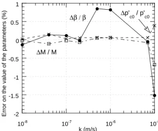
As previously done, two reference pressuremeter curves are calculated, the first one in fully drained conditions and the other in partially undrained conditions for k = 5x10-7 m.s-1 and the parameters values indicated in Table 8. Then, the value of the permeability is changed and the optimization procedure restarted. The values of β, M and p’c0 thus

optimized are of course different from the reference values. The discrepancy is reported in Figure 7 in the case of an equal weight given to the two pressuremeter curves. The error greatly increases when the permeability is underestimated or overestimated by a factor 10. The plastic compressibility β is the most dependent parameter to the value of the permeability.

To circumvent these shortcomings, two solutions are envisaged. The first idea is to enrich the experimental data with a third pressuremeter test carried out in different drainage conditions than the two first tests. No improvement in the parameter estimates is observed. The second idea is to numerically and arbitrarily provide a more important weight to the test carried out in fully drained conditions. As shown in Figure 8, this second option reveals a clear improvement of the optimization results since the error is lower than 2 % whereas the permeability is changed by a factor 100.

5 CONCLUSIONS

The theoretical issue of identification of the plastic compressibility parameter β = λ - κ is addressed in the framework of the Cam-Clay formulation. In that exercise, numerical simulations show that :

1 The value of any parameter, provided that it clearly influences the pressure versus displacement curve at the pressuremeter cavity wall, can be determined by inverse analysis of a unique pressuremeter test, whatever the drainage conditions may be.

2 The values of two parameters, among the plastic compressibility β, the critical state line slope M and the preconsolidation pressure p’c0 can be

simultaneously identified from a unique pressuremeter test carried out in drained conditions. The fourth key factor, the shear modulus G, can be calculated from the slope of an unloading – reloading loop performed during the test.

3 Assuming the value of the soil permeability k, the simultaneous identification of β, M and p’c0 can

be achieved from inverse analysis of two pressuremeter tests carried out in distinct drainage conditions.

4 Because of uncertainty about the value of the permeability k, it is recommended to numerically give a more important weight to the test in drained conditions than to the test in fully or partially undrained conditions. In such a case, the error on the permeability estimate has a slight effect on the optimized parameters.

The feasibility of the inversion scheme is proved. However, it must be confronted to real experimental data and their corollary : spatial variability of mechanical and hydraulic properties, experimental uncertainty, anisotropic fabric of the soil… Strong assumptions are also considered. In particular, no viscous effect and no over-consolidation are taken into account in this paper. Nevertheless ongoing developments show that the effect of the plastic compressibility decreases while the over-consolidation ratio increases. This could be a limitation to the application of the inverse analysis.

6 REFERENCES

Bahar, R. 1992. Analyse numérique de l’essai pressiométrique: application à l’identification de paramètres de comportement des sols. Ph.D. Thesis, Ecole Centrale Lyon

(in french).

Cambou. B. & Bahar R. 1993. Use of pressuremeter tests to define the intrinsic parameters of soil behavior. Rev. Franc.

Géotech. 63: 39-50.

Fukagawa, R., Fahey, M. & Ohta, H. 1990. Effect of partial drainage on pressuremeter test in clay. Soils and

Foundations 30(4): 134-146.

Houlsby, G.T. & Carter, J.P. 1993. The effect of pressuremeter geometry on the results of tests in clay. Géotechnique 43(4): 567-576.

Marchina, P., Brousse, A., Fontaine, J., Dano, C. & Alonso, C. 2004. In situ measurement of rock compressibility in a heavy oil reservoir. SPE International Thermal Operations

and Heavy Oil Symposium, Itohos 2004, Bakersfiled,

California, paper n°86940.

Pilvin, P. & Cailletaud, G. 1994. Identification and inverse problems related to material behavior. In Inverse Problems

in Engineering Mechanics, Balkema, Rotterdam, 79-86.

Rangeard, D., Zentar, R., Hicher, P.Y. & Moulin, G. 2002. Permeability effect on pressuremter test results. Eight Int.

Symp. Num. Mod. Geomech. (NUMOG VIII), Rome:

619-625.

Rangeard, D., Hicher, P.Y. & Zentar, R. 2003. Determining soil permeability from pressuremeter tests, Int. J. Numer.

Anal. Meth. Geomech. 27: 1-24.

Roscoe, K.H. & Burland, J.B. 1968. On the generalized stress-strain behaviour of “wet” clay. Engineering Plasticity, Cambridge University Press, 535-609.

Zentar, R. , Moulin, G. & Hicher, P.Y. 1998. Numerical analysis of pressuremeter test in soil. In proceedings of 4th

European Conference on Numerical Methods in Geomechanics (NUMGE), Udine: 593-600.

Zentar, R., Hicher, P-Y. & Moulin, G. 2001. Identification of soil parameters by inverse analysis. Computers and

Geotechnics, 28(2): 129-144. -20 0 20 40 60 80 10-8 10-7 10-6 10-5 E rr o r o n t h e v a lu e o f th e p a ra m e te r (% ) k (m/s) ∆β / β ∆p' c0 / p'c0 ∆M / M

Figure 7. Effect of an erroneous estimate on k (equal weights given to the curves in drained and partially undrained conditions). -2 -1.5 -1 -0.5 0 0.5 1 10-8 10-7 10-6 10-5 E rr o r o n t h e v a lu e o f th e p a ra m e te rs ( % ) k (m/s) ∆β / β ∆p'c0 / p'c0 ∆M / M

Figure 8. Effect of an erroneous estimate on k (different weights given to the curves in drained and partially undrained conditions).