Endogenizing leadership in the tax competition race

HAL Id: halshs-00492105

https://halshs.archives-ouvertes.fr/halshs-00492105

Submitted on 15 Jun 2010

HAL is a multi-disciplinary open access archive for the deposit and dissemination of sci-entific research documents, whether they are pub-lished or not. The documents may come from teaching and research institutions in France or abroad, or from public or private research centers.

L’archive ouverte pluridisciplinaire HAL, est destinée au dépôt et à la diffusion de documents scientifiques de niveau recherche, publiés ou non, émanant des établissements d’enseignement et de recherche français ou étrangers, des laboratoires publics ou privés.

Endogenizing leadership in the tax competition race

Hubert Kempf, Grégoire Rota-Graziosi

To cite this version:

Hubert Kempf, Grégoire Rota-Graziosi. Endogenizing leadership in the tax competition race. 2010. �halshs-00492105�

Documents de Travail du

Centre d’Economie de la Sorbonne

Endogenizing leadership in the tax competition race

Hubert KEMPF, Grégroire ROTA-GRAZIOSI 2010.39

Endogenizing leadership in the tax competition race.

1

Hubert Kempf and Grégoire Rota Graziosi

:

Mail address: Centre d’Economie de la Sorbonne, Université Paris-1 Panthéon-Sorbonne, 65 boulevard de l’Hôpital, 75013 Paris, France.

Email: hubert.kempf@univ-paris1.fr ‡: CERDI-CNRS, Université d’Auvergne,

Mail address: CERDI-AUREDI,

65 boulevard François Mitterrand, 63000 Clermont-Ferrand, France Email: gregoire.rota_graziosi@u-clermont1.fr

May 25, 2010

1_{Grégoire Rota-Graziosi thanks the research program "Gouvernance internationale,}

univer-salisme et relativisme des règles et institutions" (Université d’Auvergne) for providing financial support for this research. We are very grateful to participants to seminars at University of Clermont-Ferrand (CERDI ), University Paris 10 (EconomiX) and to meetings of the Interna-tional Atlantic Economic Association (Montreal), Public Choice Society (Las Vegas), and Public Economic Theory (Galway).

Résumé

Dans cet article, nous étendons l’approche traditionnelle de la concurrence fiscale horizontale en endogénéisant le moment des décisions faites par les pays en concurrence. Nous montrons que les équilibres parfaits en sous-jeux correspondent aux deux équilibres de Stackelberg, ce qui engendre un problème de coordination. Pour résoudre ce problème, nous considérons une spécification quadratique de la fonction de production, et nous recourrons à deux critères de sélection d’un équilibre : la risque-dominance et la Pareto-dominance. A l’équilibre ainsi sélectionné, la moins productive (la plus petite) juridiction mène et renonce à l’avantage de second-joueur. Nous obtenons ainsi deux autres résultats : (i) la pression à la baisse est moindre qu’on ne le pense généralement ; (ii) la règle selon laquelle le grand pays fixe un taux plus élevé ne tient pas toujours.

JEL Codes: H30, H87, C72.

Abstract

In this paper we extend the standard approach of horizontal tax competition by endoge-nizing the timing of decisions made by the competing jurisdictions. Following the literature on the endogenous timing in duopoly games, we consider a pre-play stage, where jurisdictions commit themselves to move early or late, i.e. to fix their tax rate at a first or second stage. We highlight that at least one jurisdiction experiments a second-mover advantage. We show that the Subgame Perfect Equilibria (SPEs) correspond to the two Stackelberg situations yielding to a coordination problem. In order to solve this issue, we consider a quadratic specification of the production function, and we use two criteria of selection: Pareto-dominance and risk-dominance. We emphasize that at the safer equilibrium the less productive or smaller jurisdiction leads and hence loses the second-mover advantage. If asymmetry among jurisdictions is sufficient, Pareto-dominance reinforces risk-Pareto-dominance in selecting the same SPE. Three results may be deduced from our analysis: (i) the downward pressure on tax rates is less severe than predicted; (ii) the smaller jurisdiction leads; (iii) the ‘big-country-higher-tax-rate’ rule does not always hold. JEL Codes: H30, H87, C72.

Key-words: Endogenous timing; tax competition; first/second-mover advantage; strategic com-plements; Stackelberg; Risk dominance.

1

Introduction

Tax competition is often seen as characterized by a downward pressure on tax rates, leading to under-provision of public goods (dubbed “race to the bottom”). This result has been obtained using models that formalize tax competition through a Nash equilibrium with simultaneous moves (see Zodrow and Mieszkowski (1986), Wilson (1986) or Wildasin (1988)).1

In this paper, we challenge this result by endogenizing the timing of decisions by fiscal authorities. The assumption of simultaneous moves of countries when deciding their tax policy, is largely accepted. But, as remarked by Schelling (1960), the viability of the equilibrium with simultaneous moves is dubious as soon as countries’ commitment is considered. An obvious way to commit is to decide before the others. Very few articles in the literature on international tax competition consider the case where tax decisions are sequential:2 _{Gordon (1992), Wang (1999) and to a smaller extent Baldwin and Krugman}

(2004). The first author considers double-taxation conventions between countries. He establishes that capital income taxation can be sustained if the dominant capital exporter country acts as a Stackelberg leader by choosing its tax policy first. Following Kanbur and Keen (1993) who focus on commodity taxation, Wang (1999) assumes that the larger country behaves as a Stackelberg leader. Baldwin and Krugman (2004) highlight the role of economies of agglomeration to explain why tax rates remain higher in the core country than in the periphery, by assuming that the core country moves first. In the empirical literature on tax competition too, few papers deviate from the simultaneous tax competition assumption (see Altshuler and Goodspeed (2002) or Redoano (2007)).

The preceding theoretical works which consider a Stackelberg configuration assume an exogenous timing, each jurisdiction or country having its predetermined role as leader or

1_{This approach has been extended in many directions by taking into account the difference among}

countries in their size or their initial endowments, by studying several tax instruments, by considering Leviathan governments, and so on. See for instance the surveys of Wilson (1999) or Wilson and Wildasin (2004) among the most recents.

2_{Several recent papers on fiscal federalism consider a Stackelberg game where the central}

govern-ment leads. However, the induced vertical tax competition is not encompassed in the definition of tax competition by Wilson and Wildasin (2004). Moreover, the sequence of moves is assumed to be given.

follower.3 _{Given this background, the aim of this paper is twofold: firstly, going beyond the}

study of the Stackelberg equilibrium, we analyze the endogenous timing of tax setting and its consequences on the final equilibrium, which becomes a Subgame Perfect Equilibrium (SPE); secondly, since there are several SPEs, we solve the coordination issue that appears by using the notions of Pareto and risk dominance. This allows us to identify the leader respectively at the efficient equilibrium and at the safest one.

Our analysis is grounded on the standard approach to horizontal tax competition proposed by Wildasin (1988), as formalized by Laussel and Le Breton (1998). This model presents the advantage of focusing exclusively on strategic interactions. Moreover, Laussel and Le Breton (1998) rigorously establish the condition of existence and uniqueness of a Nash equilibrium in the canonical tax competition game.4 Following the literature on endogenous timing in duopoly games initiated by d’Aspremont and Gerard-Varet (1980) and Gal-Or (1985), we consider the two-period action commitment game proposed by Hamilton and Slutsky (1990): each country has to move in one of two periods; if one player chooses to move early, i.e. to fix its tax rate at the first period, while the other moves late, the latter behaves as a Stackelberg follower, the former as a leader; otherwise, choices of tax rates are simultaneous, and countries play the standard tax competition game. This kind of game, which has been called “leadership game” or “commitment game” has been mainly developped in Industrial Organization.5 _{Our approach is close to}

van Damme and Hurkens (2004) and Amir and Stepanova (2006), who develop models

3_{For instance, Wang (1999) writes (p. 974):}

"It is natural and conceivable that, in a real-world situation of tax-setting, the large region moves first and the small region moves second."

4_{The issue of equilibrium existence, a fortiori uniqueness, is seldom tackled in the tax competition}

literature. Bucovetsky (1991), Wildasin (1991) or Wilson (1991) specify their respective model so as to have simple (generally linear) best reply curves. More recently, except Laussel and Le Breton (1998), we can mention the works of Bayindir-Upmann and Ziad (2005), Rothstein (2007) or Petchey and Shapiro (2009): Bayindir-Upmann and Ziad (2005) use the concept of a second order locally consistent equilibrium, which is less general than the Nash equilibrium; Rothstein (2007) considers ad valorem taxes instead of unit taxes; Petchey and Shapiro (2009) develop a dual approach, where countries minimize their policies’ costs.

5_{This framework is also used in the international trade literature (Syropoulos (1994),}

Raimondos-Møller and Woodland (2000)) and in public economics (?, where we propose a taxonomy of international interactions depending on the sign of the spillovers and the nature of interactions).

of endogenous moves in Bertrand duopoly game where firms’ strategies, i.e. prices, are complements.

We consider three “basic games” depending on the sequence of moves: one static and two Stackelberg games. In these games inspired from Wildasin (1988) and Laussel and Le Breton (1998), tax rates are strategic complements.6 _{This property has been}

widely documented in empirical works on countries’ reaction functions (see Devereux, Lockwood, and Redoano (2008) for instance). Morever, besides its realism, this property involves the supermodularity of the standard tax competition game, which insures the existence of equilibria. We rank the equilibrium tax rates obtained for the three basic games, and show that the standard tax competition equilibrium (simultaneous moves) leads to the lowest rates. We highlight a second-mover advantage for at least one of the two countries, which is consistent with the strategic complementarity of the tax rates. We turn into the timing game proposed by Hamilton and Slutsky (1990). The Subgame Perfect Equilibria (SPEs) correspond to the two Stackelberg situations. These equilibrium tax rates are unambiguously superior to these determined in the simultaneous Nash game. The downward pressure on tax rates is less strong than predicted in the standard tax competition analysis.

Since we obtain two SPEs, a new issue appears which concerns the coordination among equilibria: which country chooses to move first? To answer, we determine the conditions under which Pareto (or payoff) dominance of one SPE is garanteed. However, this criterion fails to apply for all possible situations. It requires sufficient asymmetry among countries. Beyond the Pareto criterion, we consider the notion of risk-dominance as defined by Harsanyi and Selten (1988) to establish which equilibrium is the more secure.7 _{Both the}

Pareto- and risk-dominance criteria support the view that the smaller (less productive) country leads the tax competition, thus losing the “second-mover advantage”. In other words, leading the competition does not translate into a “small country” advantage (see

6_{Bulow, Geanakoplos, and Klemperer (1985) coined the terms “strategic substitutes” and “strategic}

complements” to define the cases of downward- and upward-sloping reaction functions, respectively.

7_{We consider quadratic production functions usually used in the literature, because the use of the}

Wellisch (2000)). Indeed, we establish that the “big-country-higher-tax-rate” rule does not always hold, that is the smaller country may fix an higher tax rate. Our findings are direct implications of the existing strategic complementarity in the tax competition race. The rest of the paper is organized as follows: section 2 presents the basic framework and the three simple games depending on the simultaneity or sequentiality of country’s moves; in section 3, we determine the SPEs by ranking the tax rates in the different games, highlighting a second-mover advantage in the extended game, and solving this; in section 4, we consider the coordination issue among the two possible SPEs, and we use the Pareto-dominance and risk-dominance criteria to go beyond this issue; section 5 concludes.

2

Basic Framework

We consider a two-country economy where capital is mobile and the two fiscal authorities set capital taxes. The model is similar to the one proposed by Laussel and Le Breton (1998) as these authors provide a rigorous analysis of the existence and the uniqueness of a Nash equilibrium in a tax competition game inspired from Wildasin (1988). Our main results (Propositions 1 and 2) are based on the strategic complementarity of tax strategies, or in other terms on the supermodularity of the tax competition game.

2.1

The model

The two jurisdictions, or countries, are denoted by A and B. A single homogeneous private good is produced locally. This good can either be consumed or used as an input into the provision of the local public good. The production function used in Country i, denoted by eFi(Ki, Li), where Ki is the amount of mobile production factor (capital) and

Li the amount of fixed production factor (labor or land), is supposed to be homogenous of

degree 1. Assuming an equal endowment in the fixed factor for each country normalized to 1: LA= LB = 1, the production function of private goods in Country i can be rewritten

on the function Fi(Ki):

Fi0(Ki) > 0 > Fi00(Ki) ,

Fi00(0) > −∞,

F_i000(.) _{≥ 0.} (1)

These assumptions ensure the existence of a Nash equilibrium.

In contrast to Laussel and Le Breton (1998) who restrict themselves to the symmetric case, we introduce some asymmetry among countries by considering different production functions (FA(.)6= FB(.)). Several other formalizations of asymmetry are available in the

literature: Bucovetsky (1991) assumes that countries differ by their size; Peralta and van Ypersele (2005) consider different individual capital endowments. However, the choice of the nature of asymmetry would not affect our results, which are based on the property of strategic complementarity of tax rates. In section 4, we establish a parallel between the less productive country and the smaller country on the ground of the arguments of capital elasticity or ex ante lowly endowed country.

Each country finances its public expenditure by means of a per unit tax on capital at rate ti and a per unit tax on labor or land (a fixed production factor) at rate τi.

The availability of a non-distorting tax (τi) on an immobile factor which is supplied

inelastically, allows countries to optimally provide the public good (gi). We do not consider

the underprovision issue of the public good in order to focus exclusively on the nature of competition and its impact on tax rates. The representative wage earner in Country i may be described by the following utility function: Ui(xi, gi) = xi + gi, where xi denotes

his consumption of private goods and corresponds to his net income.8 _{As Laussel and}

Le Breton (1998) we assume that this net income derives from the fixed factor only. Thus, we have: xi = wi − τi, where wi denotes the earned wage, equal to the marginal

productivity of labor. The government budget is balanced: gi = τi+ tiKi. We define the

8_{Given the linearity and separability properties of the utility function, the public good plays no role}

welfare function of Country i as the sum Wi of the fixed factor income and the capital

tax income:9

Wi(ti, tj) = Fi(Ki)− KiFi0(Ki) + tiKi. (2)

The capital is perfectly mobile between the jurisdictions and we assume an initial level of total capital equal to K. The market clearing conditions involve:

⎧ ⎪ ⎨ ⎪ ⎩ F0 A(KA)− tA= FB0 (KB)− tB KA+ KB = K (3)

In order to turn down the “pathological” case, where there is a continuum of Nash equi-libria satisfying F0

i (Ki)− ti = 0, we assume that Fi(.)and K are such that the following

inequality holds:10

∀i = A, B, ∀Ki ∈

£

0, K¤, F_i0(Ki)− ti > 0. (4)

This second condition means that the net capital return is strictly positive. Combined with condition (1), it guarantees the uniqueness of the studied Nash equilibrium.

From (3), it is immediate to get that: ∂Ki ∂ti = 1 F00 A(KA) + FB00(KB) = ∂Kj ∂tj =₋∂Ki ∂tj < 0. (5)

The stock of capital in Country i is decreasing in its tax rate (ti) and increasing in the

9_{This assumption which is also advanced by Hindriks, Peralta, and Weber (2008) is restrictive, since}

it means that the capital owners are absent in the objective function of the government. However, Laussel and Le Breton (1998) provide two possible interpretations of a such restriction, which are consistent with Wildasin (1988): it can be justified as a partial equilibrium, or it corresponds to a political economy view, focusing on the median voter. This second view is supposed to reflect the high concentration of countries’ capital distribution.

10_{We thus restrict the equilibrium to be an interior solution. The case of capital net return equal to}

tax rate of the other country (t_j6=i).11 _{Notice that tax externalities are always positive as:} ∂Wi(ti, tj) ∂tj =−KiFi00(Ki) ∂Ki ∂tj + ti ∂Ki ∂tj > 0. (6)

Further, we can prove the following

Lemma 1 Under assumption (1), tax rates are strategic complements.

Proof. See Appendix A.1.

The explanation is simple: when government j increases its rate, it alleviates the competitive pressure on governement i as this decision reduces the incentive of capital to migrate from i to j. Therefore the marginal utility derived from an increase of the tax rate set by governement i is increasing since it generates more revenues and finances more additional public good. In other words, the second-order cross-derivatives of Wi(ti, tj)

are positive when ti is set optimally.

The strategic complementarity property of tax setting functions is crucial for our analy-sis. Several recent works focusing on the estimation of the fiscal reaction functions in an international or federal context support the view that fiscal interactions exist and high-light positive slope reaction functions among countries or jurisdictions (see for instance Revelli (2005), Devereux, Lockwood, and Redoano (2008)).

In the following subsections, we will study three different games, depending on the sequence of the countries’ tax-setting. We denote GN _{the game where both countries}

choose simultaneously their tax rate; GAthe game where Country A leads and Country B follows; and GB the game where Country B leads.

2.2

Simultaneous game

¡

G

¢

At the simultaneous non-cooperative equilibrium each country chooses its own tax rate without taking into account the externalities on the other country. We denote by¡tN

A, tNB

¢ the Nash equilibrium of this game. This pair must satisfy the following set of definitions:

11_{Since F}00

⎧ ⎪ ⎪ ⎨ ⎪ ⎪ ⎩ tN A ≡ arg max tA∈[0,1] WA(tA, tB) , tB given tN B ≡ arg max tB∈[0,1] WB(tA, tB) , tA given.

Let us define the function Φi(ti, tj)by:

Φi(ti, tj) = ti+ KiFj00(Kj) , j 6= i. (7)

As shown in Appendix A.1, the first-order conditions (FOCs) obtain: ⎧ ⎪ ⎨ ⎪ ⎩ ΦA ¡ tN_A, tN_B¢∂KA ∂tA = 0 ΦB ¡ tNB, tNA ¢∂KB ∂tB = 0 or equivalently, since ∂KA ∂tA 6= 0 from (5), 12 ⎧ ⎪ ⎨ ⎪ ⎩ ΦA ¡ tNA, tNB ¢ = 0 ΦB ¡ tN B, tNA ¢ = 0. (8)

Under assumption (1), Laussel and Le Breton (1998) establish the existence of the Nash equilibrium. Condition (4) involves the uniqueness of this equilibrium by ruling out the “pathological” case. In Appendix A.1, we show that dtj

dti < 1, which means here that

the best-reply correspondences are contractions. This is another way to guarantee the existence and the uniqueness of a Nash equilibrium (see Vives (1999), p. 47).

2.3

Stackelberg games

G

and

G

There are two Stackelberg games depending on the identity of the leader. In the game Gi_,

we assume that Country i “leads”, that is fixes first its tax rate, and Country j chooses

12_{The second-order conditions (SOCs) are satisfied at} ¡_tN A, tNB ¢ : ∂2_W i(ti, tj) ∂t2 i =∂Φi(ti, tj) ∂ti ∂Ki ∂ti + Φi(ti, tj) ∂2_K i ∂t2 i < 0, since ∂Φi(ti,tj) ∂ti > 0 and Φi ¡ tN_i , tN_j ¢= 0.

its own level tj.

Applying backward induction, we first consider the maximization program of Country j when it acts as the follower. It is given by:

tF_j (ti)≡ arg max

tj∈[0,1]

Wj(tj, ti)

The FOC of the follower obtains

Φj

¡

tF_j (ti) , ti

¢

= 0 (9)

We turn into Country i’s maximization program, when it acts as the leader. It is given by: tLi ≡ arg max ti∈[0,1] Wi ¡ ti, tFj (ti) ¢ The corresponding FOC obtains

Φi ¡ tL_i, tF_j ¡tL_i ¢¢+¡KiFi00(Ki)− tLi ¢ dtF j dti = 0. (10)

From the strategic complementarity of tax rates, we deduce that the second term of equation (10) is negative. The first term is positive. This property will allow us to rank the equilibrium tax rates in the next subsection.

2.4

Comparison of the equilibrium tax rates

We show that these equilibria generate different solutions and the tax rates obtained in a game with leadership are higher than the rates obtained in the Nash game, when the two authorities play simultaneously. This comes from the fact that tax rates are strategic complements: an increase in the rate fixed by the other government leads a government to increase its own rate.

tax rates.13

Lemma 2 For non identical countries, Nash tax rates are always lower than the tax rates obtained in a sequential game. Moreover, there are three possible rankings of the levels of tax rates: ⎧ ⎪ ⎨ ⎪ ⎩ tN A < tFA< tLA tN B < tFB < tLB , ⎧ ⎪ ⎨ ⎪ ⎩ tN A < tLA < tFA tN B < tFB < tLB or ⎧ ⎪ ⎨ ⎪ ⎩ tN A < tFA< tLA tN B < tLB < tFB.

In the case of identical countries, the following ranking obtains:

tN < tF < tL.

Proof. See Appendix A.2.

Consistent with the strategic complementarity property and the existence of positive externalities, tax rates in any Stackelberg equilibrium are higher than the rates obtained at the Nash equilibrium. When the leader, say A, increases its tax rate relative to the Nash equilibrium value, it induces the follower, B, to increase its own tax rate because of the strategic complementarity property. In turn, this increases the leader’s payoff be-cause of the positive externality induced by tax decision, and captured by the sign of ∂Wi(ti, tj) /∂tj(> 0). Hence we get tLA> tNA and tFB > tNB.In other words, the presence of

a leader in the tax competition race mitigates the “downward pressure” feature obtained in the Nash equilibrium.14

If the two countries are identical (same production function), the ranking implies that that the leader taxes more than the follower, as it is more able to resist the downward pressure on tax rates. If the two countries are sufficiently similar (close productivity schedules), they adopt similar behaviors if leading. By a continuity argument, the same ranking applies and we get tN

A < tFA < tLA and tNB < tFB < tLB.

13_{For the rest of the paper, we will use the following notation: t}F i ≡ tFi

¡ tL_j¢.

However if the two countries are sufficient dissimilar in terms of production perfor-mances, it may happen for instance that tF

A > tLA and tFB < tLB. For a sufficient degree of

asymmetry in the production functions, the interaction effects are much stronger from B to A, than from A to B. Then tLA is very close to tNA and tLB is very far from tNB as well as

tF

A from tNA. Therefore we get the two other possible rankings.

This explains the obtained possible rankings. Remark then that no combination of production functions can lead to the case where we have both tF

A > tLA and tFB > tLB.

3

Identifying the leader in the tax competition race.

These results imply that the existence and identity of a leader matter a lot in the tax competition race. Hence we would like to know the identity of the leader if it exists: is it Country A or B? To answer this question, we turn to the endogenization of moves, using a timing game. In the first stage of the timing game, the two players, here the two authorities of the jurisdictions, decide on their preferred role. They may decide they want to play “Early” or “Late”. Depending on the outcome of this stage, one of the three games described above is selected and processed. Following Hamilton and Slutsky (1990) and Amir and Stepanova (2006) we study the Subgame Perfect Equilibria of this timing game. First, we highlight the presence of a second-mover advantage. This allows us to deduce the Subgame Perfect Equilibria.

3.1

Second-mover advantage

We define the notions of “first-” and “second-mover advantage” as follows:

Definition 1 Country i has a first (second)-mover advantage if its equilibrium payoff in the Stackelberg Game in which it leads (follows) is higher than in the Stackelberg Game in which it follows (leads).

Proposition 1 At least one country has a second-mover advantage in the tax competition race.

Proof. See Appendix A.3.

When tN

i < tFi < tLi for both countries, there is a second-mover advantage for both

countries as both prefer to follow. Consider Country i, acting a follower. By decreasing its tax rate ¡tFi < tLi

¢

, when Country j sets tLj, it attracts more capital. Moreover, since

tFj < tLj, it benefits as a follower (rather than a leader) from the higher tax rate set by

Country j acting as a leader, which reorients capital towards the follower. In case of identical countries, both countries have a second-mover advantage.15 _{When t}N

i < tLi < tFi

and tN

j < tFj < tLj, only Country i prefers to follow, as the previous reasoning applies only

to this country.

3.2

A Timing Game

In order to address the existence and identity of a leader, we shall endogenize the sequence of moves by resorting to a timing game, following the seminal study of Hamilton and Slutsky (1990).

This game, which we denote by eG, is defined as follows. At the first or “preplay” stage, players simultaneously and non-cooperatively decide whether to move “early” or “late”. The players’ commitment to this choice is perfect. The timing choice of each player is announced at the end of the first stage. The second stage corresponds to the relevant tax competition game studied in the previous section, which is deduced from the timing decision at the first stage: the game ¡GN¢ _{if both players choose to move early or late;}

the Stackelberg game ¡GA¢ if Country A chooses to move early (strategy Early) while Country B chooses to move late (strategy Late); the Stackelberg game¡GB¢if Country B chooses to move early (strategy Early) while Country A chooses to move late (strategy

15_{When the two countries are identical, that is when F}

i(K) = Fj(K) , it is immediate to derive from

Late).16 _{The game eG may be reduced to a single-stage game, which has the following} normal form: Country B Early Late Country A Early WN A, WBN WAL, WBF Late WF A, WBL WAN, WBN where WiN ≡ Wi ¡ tNi , tNj ¢ , WiL≡ Wi ¡ tLi , tFj ¡ tLi ¢¢ and WiF ≡ Wi ¡ tFi ¡ tLj ¢ , tLj ¢ .

From the preceding normal form of the game eG, we obtain the following Proposition:

Proposition 2 (i) The Subgame Perfect Equilibria (SPEs) of the timing game are the Stackelberg Equilibria.

(ii) Moving sequentially instead of simultaneously is Pareto-improving for both countries. Proof. See Appendix A.4.

Since tax rates are strategic complements, there are two possible Stackelberg equilibria corresponding to the timing game eG. This comes from the fact that in any case, both the first- and second-movers are better off than under a Nash equilibrium: tax externalities are always positive and at the SPEs, the tax rates are in both countries superior to those established at the simultaneous Nash equilibrium, i.e. in the standard tax competition game (Lemma 2).17

We highlight that the SPEs are Pareto-superior to the simultaneous Nash Equilibrium (W_iF,L > WN

i ). The “downward pressure” is weaker than predicted in the standard

tax competition model since tax rates are always higher in the sequential games: both

16_{An other option exists in the literature on endogenous timing when both players choose to lead.}

Indeed, Dowrick (1986) and more recently van Damme and Hurkens (1999) consider a Stackelberg warfare, where both countries would choose their strategy as leader. In contrast, Hamilton and Slutsky (1990) or Amir and Stepanova (2006) apprehend this situation as the static Nash game. Hamilton and Slutsky (1990) emphasize that Stackelberg warfare can occur only through error, since the underlying strategy of one player is not consistent with the other player’s strategy.

17_{Notice that the equilibria studied in the literature on tax competition is not commitment robust.}

Extending the approach of Rosenthal (1991), van Damme and Hurkens (1996) establish that a Nash Equilibrium is commitment robust if and only if no player has a first-mover incentive, that is no player prefers to lead than to play the simultaneous game. In Appendix A.2, we highlight that both countries always have a first-mover incentive.

countries have a common interest in avoiding the Nash tax rates, and they can do so by resorting to non-synchronous moves, that is by accepting that one of them leads the tax competition race.

4

A coordination issue

A new issue appears due to the multiplicity of SPEs of eG: how to select one of the two possible solutions? There is a coordination issue. To solve this issue, we can resort to two criteria in order to rank the SPEs: the Pareto-dominance and the risk-dominance criteria. By so doing, we follow the deductive selection principle, that is we assume that players hold beliefs consistent with the selection criterion.18 _{Harsanyi and Selten (1988)}

define the risk-dominance criterion as follows:

Definition 2 An equilibrium risk-dominates another equilibrium when the former is less risky than the latter, that is the risk-dominant equilibrium is the one for which the product of the deviation losses is the largest.

In our framework, equilibrium (Early, Late) (Country A leads, Country B follows) risk-dominates equilibrium (Late, Early) if the former is associated with the larger prod-uct of deviation losses, denoted by Π. More formally, the equilibrium (Early, Late) risk-dominates (Late, Early) if and only if

Π _≡¡W_AL_{− WA}N¢ ¡W_BF _{− WB}N¢₋¡W_AF _{− WA}N¢ ¡W_BL_{− WB}N¢> 0. (11)

An intuition for the use of this criterion is as follows. Suppose for simplicity that WF

A − WAN = WBF − WBN. Then the threat of reverting to the Nash equilibrium when

Country A acts as a leader is bigger than the similar threat for Country B: WAL− WAN =

WBL− WBN. In other words, Country A has more to lose in case of inconsistent choices.

18_{No attempt is made to explain how decision makers acquire these beliefs. This approach contrasts}

with the inductive selection principle, which uses learning and evolutionary dynamics to predict the selection of an equilibrium.

This makes it more vulnerable to pressures from Country B than the converse. Knowing this, Country B chooses “Late” anticipating that Country A will not choose “Late” and which would lead to Nash and the higher loss ¡WAL− WAN

¢ .

As stressed by Amir and Stepanova (2006), a resolution for risk-dominance does not appear possible without using a precise specification of the problem.19 _{To apply this}

criterion to the tax competition problem, we consider a quadratic production function, already used in the relevant literature:20

Fi(K) = (a− biK) K. (12)

Ex ante (before the tax competition game starts), both countries are endowed with the same amount of capital (K/2). When bA > bB, firms in Country A are less productive

than in Country B. For a given pair of parameters (bA, bB), the tax rates and the capital

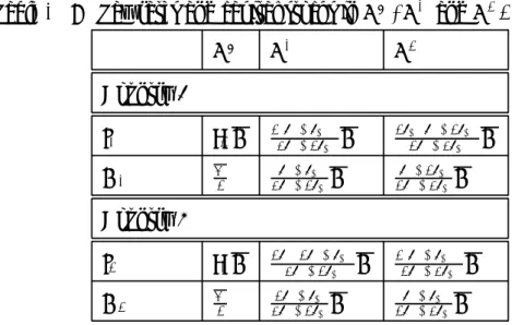
stocks at the equilibria of the three studied games are presented in the following table:

Table 1 : Tax rates and capital stocks in GN, GA and GB.

GN _GA _GB Country A tA bBK 2(bA+bB) 2 3bA+2bB K 2bB(bA+2bB) 2bA+3bB K KA K_{2 3b}bA_A+b_+2bB_BK _2bbA_A+2b_+3bB_BK Country B tB bAK 2bA(2bA+bB) 3bA+2bB K 2(bA+bB)2 2bA+3bB K KB K_{2 3b}2bA+bB A+2bBK bA+bB 2bA+3bBK

From the preceeding table, we can make several observations. First, if each region has the same capital endowment before tax competition occurs, we observe that no country exports capital at the simultaneous Nash equilibrium, while the leading country is always

19_{Analysing the competition among firms, these authors use a linear demand function as van Damme}

and Hurkens (1999).

20_{See for instance, Bucovetsky (1991), Grazzini and van Ypersele (2003), Peralta and van Ypersele}

a capital exporter. Second, at the simultaneous Nash equilibrium, the less productive country has the lower tax rate: bA> bB ⇔ tNA < tNB. This point results from the difference

in the capital elasticities (in absolute values): ¯ ¯ ¯εKN A/tNA ¯ ¯ ¯ = bB bA+bB < ¯ ¯ ¯εKN B/tNB ¯ ¯ ¯ = bA bA+bB. Since

Country A, being less productive, has a higher elasticity on capital in absolute value, it is more sensitive to capital mobility and thus is led to tax less. Here we echo the analysis of Bucovetsky (1991) and Wilson (1991) who establish that small jurisdictions21 _{tend to set}

lower tax rates than large ones. On the basis of capital elasticity, we can draw a parallel between size and productivity, when we consider that the smaller country corresponds to the less productive one, which we also call the ex ante lowly endowed country.

Given the definition (11) of risk-dominance, we obtain the following Proposition: Proposition 3 (i) The SPE, where the less productive country leads, risk-dominates the other equilibrium.

(ii) If the asymmetry between countries is sufficient, the safer SPE becomes Pareto-dominant.

Proof. See Appendix A.5.

This proposition implies that Country A is always selected as the leader, according to the risk-dominance criterion as long as bA > bB.22 Let us define γ as the degree of

asymmetry among the two countries: γ = bB/bA(γ < 1 means that Country A is the less

productive). When the difference in productivity is sufficiently pronounced (γ < γ_{1 ' 0.25} or γ > γ_{2 ' 4, see Appendix A.5.3), one country has a first-mover advantage, while the} other still has a second-mover advantage. The risk-dominant equilibrium becomes

Pareto-21_{Small jurisdictions or countries may be considered as ex ante lowly endowed, since their size in}

population explains directly their initial stock of capital under the assumption that each inhabitant has the same individual endowment in capital.

22_{This result is a straight criticism of the assumption made by Wang (1999) or Baldwin and Krugman}

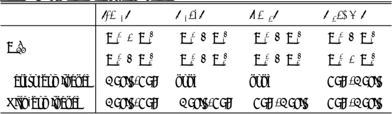
dominant. The following table summarizes the results of the preceeding Proposition:23

Table 2: Risk and Pareto dominance

γ [0, γ₁[ [γ₁, 1[ [1, γ₂[ [γ₂, +_∞[ Wk i,j WAF < WAL WBF > WBL WAF > WAL WBF > WBL WAF > WAL WBF > WBL WAF > WAL WBF < WBL

Pareto-dominance (Early, Late) none none (Late, Early) Risk-dominance (Early, Late) (Early, Late) (Late, Early) (Late, Early)

At the safer SPE, the less productive country has to move early (A for γ < γ₁, B for γ > γ₂) since it has more to lose in playing the simultaneous game than the other country. For instance, if γ < γ1, Country A increases its own tax rate compared to the Nash level,

which will trigger a larger increase in Country B tax rate because of the complementarity effect; on the other hand, if B is a leader (Early), given that A as a follower (Late) will not tend to act much, the gain of B as a leader with respect to the Nash solution, is not that large.

When the asymmetry is sufficient (γ < γ₁ or γ > γ₂), the SPE where the less pro-ductive country leads, becomes Pareto-superior to the other SPE. Indeed, for low values of bB with respect to bA (γ < γ1), the less productive country (namely A) experiments

a first-mover advantage, while the other has a second-mover advantage. By leading and fixing a higher tax rate ¡tLA > tFA

¢

, Country A encourages Country B to increase its tax rate since we have tF

B > tLB.24 Thus, Pareto-dominance reinforces risk-dominance when

countries’ asymmetry is sufficient.

Finally, our analysis invites to reconsider the “big-country-higher-tax-rate” rule, which was emphasized first by Bucovetsky (1991).25 _{Indeed, while at the simultaneous Nash}

equilibrium, the more productive, or equivalently, the larger country always sets a higher

23_{See the Appendix A.5 for a justification of the necessary condition: b < 3/4 and the definition of}

γ_k. A graphical illustration of these results is provided in the Appendix (Graph 4).

24_{From Table 1, we have t}F

B> tLB for γ <eγ, where eγ is solution of 1 − 4γ2− 2γ3= 0, eγ ≈ 0.451606. 25_{In an asymmetric model of international trade Raimondos-Møller and Woodland (2000) also establish}

the existence of situations in which the small country leads, fixing its tariff rate first and yielding to improve the welfare of both countries.

tax rate due to its relatively low elasticity of capital to the tax rate, it may set the lower tax rate at the safer SPE. More formally, for 1 > γ > √5−1₂ , we obtain tL

A> tFB.26 The less

productive (equivalently, the smaller) country may tax at a higher rate than the other country. In other terms, the ex ante advantage (in productivity or in size) enjoyed by one country allows it to reap the second-mover advantage.

5

Conclusion

Our analysis revisits tax competition by relaxing one implicit assumption generally made in the relevant literature: the simultaneity of decisions on tax rates. Inspired by several works in Industrial Organization, we developed a model where the timing of move, i.e. the tax-setting, is endogenous. Our main results hold for any form of the government’s objective function as long as tax rates are strategic complements. We established that: the tax rates are higher when countries move sequentially than when they move simulta-neously; at least one country experiments a second mover-advantage; moving sequentially is Pareto- improving; the SPEs correspond to the two Stackelberg situations yielding to a coordination issue. By specifying quadratic production functions, we solve it by applying the notions of Pareto and risk dominance. At the safer SPE, the ex ante well endowed country follows, reinforcing its ex ante advantage through the second-mover advantage. When countries’ asymmetry is sufficient, Pareto-dominance confirms risk-dominance in selecting the same SPE.

In addition to the empirical studies which would explicitly consider the dynamics of tax-setting decisions,27 further research could be considered. An immediate development

26_{Moreover, the elasticity of capital is lower in the follower country:}

¯ ¯ ¯εKF B/tFB ¯ ¯ ¯ = _b bA A+ bB <¯¯_¯εKL A/tLA ¯ ¯ ¯ = 1.

27_{Very few empirical studies have considered the order of tax-setting: Altshuler and Goodspeed (2002)}

established that European countries follow the United States when they set their tax rate; focusing on European countries only, Redoano (2007) show that large countries behave as leader. We established an inverse sequence of tax decisions at the safer equilibrium. This contradiction invites to further empirical and theoretical developments.

is to introduce the capital owners in the welfare function. New conditions for existence and uniqueness of the Nash equilibrium would be needed so as to ensure that tax rates be strategic complements and the analysis developped above applied.28 An other development would be to to consider the issue of underprovision of public goods when the timing of moves is endogenized.

References

Altshuler, R., and T. J. Goodspeed (2002): “Follow the leader? Evidence on European and U.S. tax competition,” Departmental Working Papers 200226, Rutgers University, Department of Economics.

Amir, R., and A. Stepanova (2006): “Second-mover advantage and price leadership in Bertrand duopoly,” Games and Economic Behavior, 55(1), 1—20.

Baldwin, R. E., and P. Krugman (2004): “Agglomeration, integration and tax har-monisation,” European Economic Review, 48(1), 1—23.

Bayindir-Upmann, T., and A. Ziad (2005): “Existence of equilibria in a basic tax-competition model,” Regional Science and Urban Economics, 35(1), 1—22.

Bucovetsky, S. (1991): “Asymmetric tax competition,” Journal of Urban Economics, 30(2), 167—181.

Bulow, J. I., J. D. Geanakoplos, and P. D. Klemperer (1985): “Multimarket oligopoly: strategic substitutes and complements,” Journal of Political Economy, 93(3), 488—511.

d’Aspremont, C., and L.-A. Gerard-Varet (1980): “Stackelberg-solvable games and pre-play communication,” Journal of Economic Theory, 23(2), 201—217.

Devereux, M., B. Lockwood, and M. Redoano (2008): “Do countries compete over corporate tax rates?,” Journal of Public Economics, 93(5-6), 1210—1235.

Dowrick, S. (1986): “Von Stackelberg and Cournot duopoly: choosing roles,” Rand Journal of Economics, 17(2), 251—260.

Gal-Or, E. (1985): “First mover and second mover advantages,” International Economic Review, 26(3), 649—653.

Gordon, R. H. (1992): “Can capital income taxes survive in open economies?,” Journal of Finance, 47(3), 1159—80.

Grazzini, L., and T. van Ypersele (2003): “Fiscal coordination and political com-petition,” Journal of Public Economic Theory, 5(2), 305—325.

Hamilton, J. H., and S. M. Slutsky (1990): “Endogenous timing in duopoly games: Stackelberg or Cournot equilibria,” Games and Economic Behavior, 2(1), 29—46. Harsanyi, J. C., and R. Selten (1988): A general theory of equilibrium selection in

games. MIT Press, Cambridge, MA.

Hindriks, J., S. Peralta,andS. Weber (2008): “Competing in taxes and investment under fiscal equalization,” Journal of Public Economics, 92(12), 2392—2402.

Kanbur, R., and M. Keen (1993): “Jeux sans frontieres: tax competition and tax coordination when countries differ in size,” American Economic Review, 83(4), 877—92. Laussel, D., and M. Le Breton (1998): “Existence of Nash equilibria in fiscal

com-petition models,” Regional Science and Urban Economics, 28(3), 283—296.

Peralta, S., and T. van Ypersele (2005): “Factor endowments and welfare levels in an asymmetric tax competition game,” Journal of Urban Economics, 57(2), 258—274. Petchey, J. D., and P. Shapiro (2009): “Equilibrium in fiscal competition games

from the point of view of the dual,” Regional Science and Urban Economics, 39(1), 97—108.

Raimondos-Møller, P., and A. D. Woodland (2000): “Tariff strategies and small open economies,” Canadian Journal of Economics, 33(1), 25—40.

Redoano, M. (2007): “Fiscal interactions among European countries. Does the EU matter?,” CESifo Working Paper Series CESifo Working Paper No., CESifo GmbH. Revelli, F. (2005): “On spatial public finance empirics,” International Tax and Public

Finance, 12(4), 475—492.

Rosenthal, R. W. (1991): “A note on robustness of equilibria with respect to commit-ment opportunities,” Games and Economic Behavior, 3(2), 237—243.

Rothstein, P. (2007): “Discontinuous payoffs, shared resources, and games of fiscal competition: existence of pure strategy Nash equilibrium,” Journal of Public Economic Theory, 9(2), 335—368.

Schelling, T. (1960): The strategy of conflict. Harvard University Press, Cambridge, MA.

Syropoulos, C. (1994): “Endogenous timing in games of commercial policy,” Canadian Journal of Economics, 27(4), 847—64.

van Damme, E., and S. Hurkens (1996): “Commitment robust equilibria and endoge-nous timing,” Games and Economic Behavior, 15(2), 290—311.

(1999): “Endogenous Stackelberg leadership,” Games and Economic Behavior, 28(1), 105—129.

(2004): “Endogenous price leadership,” Games and Economic Behavior, 47(2), 404—420.

Vives, X. (1999): Olipoly pricing. Old ideas and new tools. The MIT Press, Cambridge, Massachusetts.

Wang, Y.-Q. (1999): “Commodity taxes under fiscal competition: Stackelberg equilib-rium and optimality,” American Economic Review, 89(4), 974—981.

Wellisch, D. (2000): The theory of public finance in a federal state. Cambridge Univer-sity Press, New York.

Wildasin, D. E. (1988): “Nash equilibria in models of fiscal competition,” Journal of Public Economics, 35(2), 229—240.

(1991): “Some rudimetary ’duopolity’ theory,” Regional Science and Urban Eco-nomics, 21(3), 393—421.

Wilson, J. D. (1986): “A theory of interregional tax competition,” Journal of Urban Economics, 19(3), 296—315.

(1991): “Tax competition with interregional differences in factor endowments,” Regional Science and Urban Economics, 21(3), 423—451.

(1999): “Theories of tax competition,” National Tax Journal, 52(2), 269—304. Wilson, J. D., and D. E. Wildasin (2004): “Capital tax competition: bane or boon,”

Journal of Public Economics, 88(6), 1065—1091.

Zodrow, G. R.,and P. Mieszkowski (1986): “Pigou, Tiebout, property taxation, and the underprovision of local public goods,” Journal of Urban Economics, 19(3), 356—370.

A

Appendix

A.1

Proof of Lemma 1: strategic complementarity of the tax

rates

The derivation of Wi(ti, tj) with respect to ti yields:

∂Wi(ti, tj) ∂ti = −Ki F_i00(Ki) ∂Ki ∂ti + Ki+ ti ∂Ki ∂ti Using (5), we get ∂Wi(ti, tj) ∂ti = ti− KiFi00(Ki) + Ki(FA00(KA) + FB00(KB)) F00 A(KA) + FB00(KB) = £ti+ KiFj00(Kj) ¤ ∂Ki ∂ti = Φi(ti, tj) ∂Ki ∂ti , where the function Φi(ti, tj) is defined by:

Φi(ti, tj) = ti+ KiFj00(Kj) , j 6= i. We have ∂Φi(ti, tj) ∂ti = 1 +£F_j00(Kj) − KiFj000(Kj)¤ ∂Ki ∂ti , and ∂Φi(ti, tj) ∂tj =£_−Fj00(Kj) + KiFj000(Kj)¤ ∂Kj ∂tj . Under assumption (1), we deduce

∂Φi(ti, tj)

∂ti

> 0 and ∂Φi(ti, tj) ∂tj

< 0. Applying the Envelop theorem to (8) or equivalently to (9), we obtain29

dtj dti = − ∂Φj(tj,ti) ∂ti ∂Φj(tj,ti) ∂tj > 0 and dtj dti < 1. ¤

A.2

Proof of Lemma 2: ranking of the equilibrium tax rates

From the definition of the Stackelberg equilibrium, we always have: Wi¡tLi, tFj ¡ tL_i¢¢_{≡ max} ti Wi¡ti, tFj (ti)¢ > Wi¡tNi , tFj ¡ tN_i ¢¢= Wi¡tNi , tNj ¢ , (13) since tF j ¡ tN i ¢ = tN

j by definition of the follower’s maximisation program. Inequality (13) involves that

each country has a first-mover incentive.

We now show that it cannot be the case that tN j > tFj

¡ tL

i

¢

. If it were true, since ∂Wi(ti,tj)

∂tj =

29_{Note that} ∂Ki

∂ti =

∂Kj

−∂Ki

∂tjKiF

00

i (Ki) + ti∂K∂tji > 0, then the definition of the Nash equilibrium yields

Wi¡tNi , tNj ¢ ≡ max_t i Wi¡ti, tNj ¢ > Wi ¡ tL_i, tN_j ¢ > Wi ¡ tL_i, tF_j¢, which contradicts (13). Thus we always have:

tF_i > tN_i , i = A, B. (14) Since ∂Ki

∂ti < 0 and

dti

dtj > 0, we derive from the FOCs of the three different games (G

N,A,B_{) (8), (9)} and (10) that Φi ¡ tL_i, tF_j¢> Φi ¡ tN_i , tN_j ¢= Φi ¡ tF_i , tL_j¢= 0. (15) Since ∂Φi(ti,tj) ∂tj < 0 < ∂Φi(ti,tj)

∂ti , the inequalities (14) and (15) involve that we always have

tL_i > tN_i , i = A, B. (16) Moreover, inequality (15) involves

tL_i < tF_{i ⇒ t}F_j < tL_j tF_j > tL_{j ⇒ t}L_i > tF_i .

Hence, we have three possible rankings for the tax rates: ∀ (i, j) ∈ {A, B}2and i 6= j, ½ tN i < tFi < tLi tN j < tFj < tLj or ½ tN i < tFi < tLi tN j < tLj < tFj

For identical countries, we have: tL

A= tLB = tL, tFA ¡ tL B ¢ = tF B ¡ tL A ¢ = tF _{and t}N A = tNB = tN. We obtain

one possible ranking only:

tN< tF < tL. ¤

A.3

Proof of Proposition 1: second-mover advantage

• When ∀i = A, B, tN i < tFi < tLi, we have Wi¡tFi, tLj¢ > Wi¡tLi, tLj ¢ > Wi¡tLi, tFj ¢ ,

where the first inequality results from the definition of the Stackelberg equilibrium when Country i follows, and the second from the facts that tF

j < tLj and

∂Wi(ti,tj)

∂tj > 0. Each country has a

second-mover advantage. • When tN i < tLi < tFi and tNj < tFj < tLj, we have Wi¡tFi, tLj ¢ > Wi¡tLi, tLj ¢ > Wi¡tLi, tFj ¢ , by similar reasoning. Country i has a second-mover advantage.¤

A.4

Proof of Proposition 2: Subgame Perfect Equilibria

(i) For each country i, we always have by definition W_iL> W_iN. Moreover, we know that

W_iF = Wi¡tFi ¡ tL_j¢, tL_j¢ > Wi¡tNi , tLj ¢ > Wi¡tNi , tNj ¢ = W_iN.

where the first inequality results from the definition of the Stackelberg equilibrium when Country i follows, and the second from the facts that tL_i > tN_i and ∂Wi(ti, tj) /∂tj > 0. Thus, there are two SPEs which

correspond to the two Stackelberg situations. (ii) Immediate given the above inequalities.¤

A.5

Proof of Proposition 3: Risk and Pareto-dominance with a

quadratic production function

A.5.1 Restrictions on the parameters’ values (a, bA, bB andK)

The assumption of a not negative net return of capital given in (4) and the nature of tax rates, which must belong to the interval [0, 1] induce some restrictions on the parameters’ values (respectively a, bA,

bB and K). Without loss of generality, we normalize the total capital endowment to unity ¡K = 1¢.

Moreover, we assume that a = 1, bA= b and bB= γbA, with γ > 0. We obtain the following restrictions,

which induce a relationship between b and γ:30 ½ 0 < b <_4+6γ+2γ3+2γ 2 0 < γ6 1 (17) or _½ 0 < b <_3+6γ+3γ3+2γ 2 γ > 1. (18)

We may reduce these preceding restrictions to a sufficient condition on b, that is:

b < 3/4. (19)

A.5.2 Risk-dominance The deviations product is then:

Π (b, γ) = b2_{(1 + γ) (1 − γ) Q (γ) ,} where

Q (γ) = 14 + 78γ + 180γ

2_{+ 231γ}3_{+ 180γ}4_{+ 78γ5 + 14γ}6

2 (6 + 13γ + 6γ2₎3 .

Since Q (γ) > 0 for any γ respecting and , we deduce that: sign {Π (b, γ)} = sign {1 − γ}. We obtain: If γ < 1,

(A moves Late, B moves Early) Risk-dominates (A moves Early, B moves Late). If γ > 1,

(A moves Early, B moves Late) Risk-dominates (A moves Late, B moves Early).

A.5.3 Pareto-dominance

In order to establish the Pareto dominance, we compare the payoff functions at the different equilibria. We have: W_AF_{− WA}L = −1 + γ 2_{(1 + γ) (11 + 7γ)} (3 + 2γ) (2 + 3γ)2 b > 0 if and only if γ < γ1≈ 0.250419. W_BF_{− WB}L = 7 + 18γ + 11γ 2 − γ4 (3 + 2γ)2(2 + 3γ) b > 0 if and only if γ > γ2≈ 3.99331. If γ < γ₁,

(A moves Late, B moves Early) Pareto-dominates (A moves Early, B moves Late). If γ > γ₂,

(A moves Early, B moves Late) Pareto-dominates (A moves Late, B moves Early). ¤

B

Graphs

B.1

Graph 1: Reactions functions

The following graphs present the reaction functions in the case of quadratic production functions with a normalized worldwide capital (K = 1). These reaction functions are denoted tF

i (tj), since they are

established with the follower’s maximization program, but correspond also to the simultaneous Nash maximization program. (Early, Late) denotes the Stackelberg equilibrium where Country A leads and B follows. Nash HEarly,LateL HLate,EarlyL tF_AHt_BL t_BFHt_AL 0.06 0.08 0.10 0.12 tA 0.05 0.10 0.15 0.20 t_B t_AN_<t A F_Ht B L_L<t A L _{fl t} B N_<t B F_Ht A L_L<t B L Graph 1: K = 1, bA= 0, 3 and bB = 0, 45. Nash HEarly,LateL HLate,EarlyL tFAHtBL t_BFHt_AL 0.12 0.14 0.16 0.18 tA 0.05 0.10 0.15 tB tA N_< tA L_< tA F_H tB L_{L fl} tB N_< tB F_H tA L_L< tB L Graph 2: K = 1, bA= 0, 2 and bB = 0, 6.

Nash HEarly,LateL HLate,EarlyL tF_AHt_BL t_BFHt_AL 0.02 0.04 0.06 0.08 0.10 tA 0.1 0.2 0.3 0.4 0.5 t_B t_AN_<t A F_Ht B L_L<t A L _{fl t} B N_<t B L_<t B F_Ht A L_L Graph 3: K = 1, bA= 0, 6 and bB = 0, 2.

B.2

Graph 2: Pareto and Risk-dominance

The following graph illustrates Proposition 3.

g1 1

HEarly,LateL Pareto dominates

HEarly,LateLrisk-dominates

HLate, EarlyLrisk-dominates

bA

PH.L