HAL Id: hal-01093153
https://hal.inria.fr/hal-01093153
Submitted on 10 Dec 2014
HAL is a multi-disciplinary open access
archive for the deposit and dissemination of
sci-entific research documents, whether they are
pub-lished or not. The documents may come from
teaching and research institutions in France or
abroad, or from public or private research centers.
L’archive ouverte pluridisciplinaire HAL, est
destinée au dépôt et à la diffusion de documents
scientifiques de niveau recherche, publiés ou non,
émanant des établissements d’enseignement et de
recherche français ou étrangers, des laboratoires
publics ou privés.
High performances simulation of ultrasonic fields for
Non Destructive Testing
Jason Lambert, Lionel Lacassagne, Gilles Rougeron, Stéphane Le Berre,
Sylvain Chatillon
To cite this version:
Jason Lambert, Lionel Lacassagne, Gilles Rougeron, Stéphane Le Berre, Sylvain Chatillon. High
per-formances simulation of ultrasonic fields for Non Destructive Testing. Joint International Conference
on Supercomputing in Nuclear Applications + Monte Carlo, Société Française d’Energie Nucléaire,
Oct 2013, Paris, France. �10.1051/snamc/201404302�. �hal-01093153�
Joint International Conference on Supercomputing in Nuclear Applications and Monte Carlo 2013 (SNA + MC 2013)
La Cité des Sciences et de l’Industrie, Paris, France, October 27-31, 2013
High performances simulation of ultrasonic fields for Non Destructive Testing
Jason LAMBERT1*, Lionel LACASSAGNE2, Gilles ROUGERON1, Stéphane LE BERRE1, Sylvain CHATILLON1
1
CEA LIST, CEA Saclay Digiteo Labs, pc 120, 91191 Gif-sur-Yvette cédex, France
2
LRI (Laboratoire de Recherche en Informatique), UMR8623, Universite Paris-Sud 11, France
*
Corresponding Author, E-mail: [email protected] Abstract:
Ultrasonic imaging is a commonly used method to detect and identify defects in a mechanical part in nuclear applications. Nowadays massively parallel architectures enable the simulation of ultrasonic field emitted by a phased array transducer inspecting a part across a coupling medium. In this paper, regular field computation model will be discussed along its implementations on General Purpose Processors (GPP) and Graphic Processing Units (GPU).
KEYWORDS:non-destructive testing, ultrasonic simulation, general purpose processors, graphic processing units, massive parallelism
I. Introduction
Inspection simulation is used in a lot of non-destructive evaluation (NDE) application: from designing new inspection methods and probes to qualifying methods and demonstrating performances through virtual testing while developing methods. The CIVA software, developed by CEA-LIST and partners is a multi-technique platform (Ultrasonic Testing (UT), Computed Tomography and Radiographic Testing (CT-RT) Eddy-current Testing (ET), Guided Wave (GW)) used to both analyze acquisitions and to run simulations validated against international benchmark. In particular, the simulation of ultrasonic field radiated in specimen is widely used in order to design or evaluate probe potential efficiency for a given control. Thus, ultrasonic beam main characteristics such as focal spot or local direction can easily be determined. A common nuclear application is the inspection of steel pipes and nozzles, as illustrated in Figure 1. It shows the simulated ultrasonic fields in a weld between two pipes with a contact probe as opposed to a flexible phased array probe. In the second case the beam is radiated with better directionality and increased amplitude.
Figure 1 - Field simulation inside a weld with two different probes.
However, due to the potential complexity of the configurations, current semi-analytical models implemented in CIVA software, based on asymptotic developments, takes minutes to hours to run a simulation. Significant efforts are made to reduce computation times by working both on models and computational aspects. The works reported here ties in with this general approach.
Nowadays, new massively parallel architectures can empower computational software, at the expense of adapting algorithms to the specificities of those architectures to highlight and improve parallel computation steps. The exploitation of both multicore-GPP and GPU capabilities results in a new intensively parallel algorithm of simulation of UT beam. Those architectures have already been used to provide consistent speedup over wave propagation [1], or field modeling for a probe alone [2] but they have not been applied to UT field simulation yet.
The new model relies on analytical solution to the beam propagation. Its implementations on both architectures use high performances signal processing libraries (Intel MKL on GPP and NVidia cuFFT on GPU). The new model is, however, limited to canonical configurations due to the strict parallelism requirements and to the lack of genericity of analytical beam propagation.
II. Beam propagation modelization for regularity
The ultrasonic field computation relies on the pencil method, a generic approach for heterogeneous and anisotropic structures. By evaluating the ray path of the beam, from the transducer to the observation point, it is possible to evaluate the time of flight and the amplitude of the contribution of the beam using energy conservation principle on the tube. As seen in Figure 2, the beam may propagate through different materials and cross multiple interfaces: its contributions is determined by the propagation matrix obtained by
multiplying the elementary contributions of each section of the pencil with the initial contribution , as shown in equation 1 [3].
(1)
Figure 2 - Ray tube visualization
In general case, there is no simple solution to determine the ray path from the source point to the computation point. However, in isotropic and homogeneous structures, analytical methods can be used to determine ray path. In direct mode, for standard geometrical surfaces, it is possible to determine a polynomial modelizing the path following Snell-Descartes. The roots of this polynomial, whose degree vary from 4th for planar surfaces to 16th for torical surfaces, correspond to the possible solutions for the ray path. They are determined numerically, through Newton’s and Laguerre’s Method [4]. In the case of half-skip mode, ray path can only be determined analytically for planar surfaces and planar backwalls as illustrated in Figure 3, through two dimensional Newton’s method solving.
R1 c1 R2 c2 θ1 θ2 R1 c1 R2 c2 R3 c3 θ1 θ2 θ3 θ2fd
Figure 3 - Ray path determination in direct and half-skip mode
Those methods rely on a numerical resolution of analytical formulas which allow for a greater regularity benefiting to the requirements of massively parallel architectures. Moreover, as this model is dedicated only to a specific set of geometries, the propagation matrix can be fully determined preemptively thus avoiding costly matrix multiplication, for the computed modes. According to the simulated propagation mode (longitudinal or transversal), transmission and reflection Fresnel’s coefficients are computed with analytical, specialized, equations.
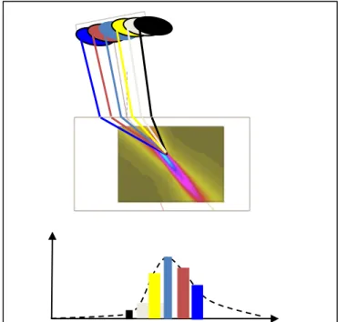
In each point field, once pencils are computed on the whole transducer, their elementary contributions are summed up to obtain the impulse response of the elastodynamic displacement, as presented in Figure 4.
Figure 4 - Formation of the impulse response at point M
The impulse response is then convoluted in the frequency domain with the reference signal to obtain the resulting signal of the modulus of displacement in each point. The results of the beam formation simulation are the image of maximum of amplitude of the modulus of displacement and the image of the corresponding time of flight. Algorithm 1 presents the generic algorithm required to compute the resulting image.
Algorithm 1 - Beam formation simulation for(P point in fieldzone) {
⃗⃗⃗⃗⃗⃗⃗⃗⃗⃗⃗⃗⃗⃗⃗⃗⃗⃗⃗⃗⃗⃗⃗⃗⃗⃗⃗⃗⃗⃗⃗⃗⃗⃗⃗⃗⃗⃗ ( ) ⃗ ( )
for(M field mode) {
for(S surface) {
for(E sensor element) {
path = analytical_path(P,E,M,S); tof = time_of_flight(path); delay = ; ⃗⃗⃗⃗⃗⃗⃗⃗⃗⃗⃗⃗⃗⃗⃗⃗⃗⃗⃗⃗⃗⃗⃗⃗⃗⃗⃗⃗⃗⃗⃗⃗⃗⃗⃗⃗⃗⃗⃗⃗⃗⃗⃗⃗⃗⃗⃗⃗⃗⃗⃗⃗⃗⃗⃗⃗⃗ = pencil_information(path); ⃗⃗⃗⃗⃗⃗⃗⃗⃗⃗⃗⃗⃗⃗⃗⃗⃗⃗⃗⃗⃗⃗⃗⃗⃗⃗⃗⃗⃗⃗⃗⃗⃗⃗⃗⃗⃗⃗ ( ) ⃗⃗⃗⃗⃗⃗⃗⃗⃗⃗⃗⃗⃗⃗⃗⃗⃗⃗⃗⃗⃗⃗⃗⃗⃗⃗⃗⃗⃗⃗⃗⃗⃗⃗⃗⃗⃗⃗⃗⃗⃗⃗⃗⃗⃗⃗⃗⃗⃗⃗⃗⃗⃗⃗⃗⃗⃗ ; } // element } // surface } // mode ⃗⃗⃗⃗⃗⃗⃗⃗⃗⃗⃗⃗⃗⃗⃗⃗⃗⃗⃗⃗⃗⃗⃗⃗⃗⃗⃗⃗⃗⃗ ( ) ⃗⃗⃗⃗⃗⃗⃗⃗⃗⃗⃗⃗⃗⃗⃗⃗⃗⃗⃗⃗⃗⃗⃗⃗⃗⃗⃗⃗⃗⃗⃗⃗⃗⃗⃗⃗⃗⃗ ( ) ( ) ; signal(t) = ‖ ⃗⃗⃗⃗⃗⃗⃗⃗⃗⃗⃗⃗⃗⃗⃗⃗⃗⃗⃗⃗⃗⃗⃗⃗⃗⃗⃗⃗⃗⃗ ( )‖ ; (Amax[P],Tmax[P]) = maximum_extraction(signal(t)); } Elementary surface Observation point Axial ray Source point Paraxial ray Solid angle
II. Implementations
In this section, choices of implementation, both on GPP and GPU architectures, will be discussed under the specificities of the hardware. It is noteworthy that the current implementations are restricted to a subset of configurations as this preliminary work is aimed at validating the model and at providing first benchmarking results. The scope of those implementations is planar surfaces and direct mode simulation.
1. GPP implementation
The GPP implementation is dedicated to take advantage of modern day GPP, composed of multiple general purpose core aimed at executing independent, heavyweight tasks. GPP disposes of two parallelism levels.
• A fine grained parallelism relying on specific SIMD instructions (Single Instruction Multiple Data) which execute the same operation on short vectors (128 to 512 bits). For example, with 128-bit vectors, a SIMD instruction can
perform simultaneously four additions on four
single-precision floating point numbers (32-bit).
• A coarse grained parallelism relying on multithreading to enable multiple logical tasks to reside simultaneously on the GPP. The OpenMP API is aimed at shared-memory parallelism: it creates a thread per GPP core, each with its own stack where local variables are located but they can also communicate through some shared variable. Its work distribution relies on a succession of sequential sections (with only one active thread) and parallel sections (with all threads active) assembled in a fork-join fashion.
In this implementation, computations are aggregated by coarse step, regrouped over the whole set of points, to even the computation load on the GPP between the cores and in order to maximize the reutilization of the data describing the simulation.
It is noteworthy that both displacement convolution and maximum extraction (relying on the determination of the maximum of the envelope of the displacement modulus) rely on Fast Fourier Transform (FFT). As this operation has been extensively studied and is not the main subject of this work, to benefit from heavily optimized FFT operation, this implementation will use the Intel® Math Kernel Library (MKL). This library offer highly vectorized FFT function to benefits from the SIMD capability of GPP cores.
However, to obtain the best performances, the size of the signal over which the FFT will be applied need to be known in advance: some coefficients can therefore be computed in advance, and then be reused several times over different signals. It is the same notion of plan as that used by cuFFT and other dedicated libraries and it is so-called descriptor in this implementation..
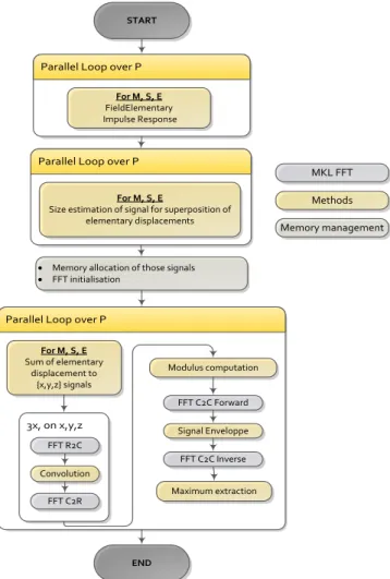
Figure 5 presents the algorithm of the GPP implementation, highlighting the chosen steps and the necessary call to the MKL with a specific step to predetermine the size of the resulting signals.
Parallel Loop over P Parallel Loop over P
Parallel Loop over P
START Modulus computation Maximum extraction MKL FFT Methods Memory management For M, S, E FieldElementary Impulse Response For M, S, E Sum of elementary displacement to {x,y,z} signals
· Memory allocation of those signals · FFT initialisation
For M, S, E
Size estimation of signal for superposition of elementary displacements END FFT C2C Forward Signal Enveloppe FFT C2C Inverse 3x, on x,y,z FFT R2C Convolution FFT C2R
Figure 5 - Algorithm of the GPP Implementation
2. GPU implementation
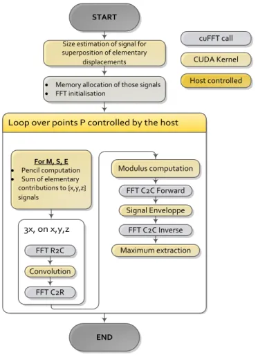
Due to the high need for computational regularity on GPU, the control flow of this implementation will aim at executing the same task over multiple data and proceed in steps, each corresponding to dedicated kernel. To benefit from highest GPU performances, kernels were developed to use single-precision floating point operations (IEEE-754). To perform signal processing operations, this implementation relies on the optimized cuFFT library which is optimized to perform efficiently on large batches of signals. This library establishes a ”plan”, consisting in the precomputed coefficients which are applied to the signals. It is most efficient when performed repeatedly on a batch of signals of the same dimensions (number of signals and signal length), to reuse a previously computed plan. The following Figure 6 illustrates the overall required computations steps detailed as follow.
The first step of the computation determines the temporal width of the resulting signal corresponding to the summation of the different elementary contributions obtained from the pencils. It combines two successive kernel calls:
• The first kernel is specialized toward direct mode; threads from a single group work collaboratively to computes the elementary displacements from pencils data before reducing temporal information. Those threads groups are spread
across the different points where field is to be computed. • The second kernel aims at reducing all those temporal information on the whole zone to obtain the global size. Due to the numerous points where signal should be determined and due to the required size of the signal, it is not possible to compute the whole UT field at once: work is divided on several slices to fit the available memory on a high end consumer grade GPU (1.5GB). The following steps will be repeated on each slice in a loop controlled by the host system.
Loop over points P controlled by the host
3x, on x,y,z
START
Size estimation of signal for superposition of elementary displacements For M, S, E · Pencil computation · Sum of elementary contributions to {x,y,z} signals Modulus computation FFT R2C Convolution FFT C2R Maximum extraction END
· Memory allocation of those signals
· FFT initialisation FFT C2C Forward Signal Enveloppe FFT C2C Inverse cuFFT call CUDA Kernel Host controlled
Figure 6 - Algorithm of the GPU implementation
The second steps begin with the summation of the elementary displacements to the corresponding signals for a given point P. The corresponding kernel is specialized by mode due to the differences in computations: longitudinal mode elementary responses result in real signals whereas transversal ones result in complex signals. This kernel organizes threads blocks in a similar fashion to the one evaluating the size of the resulting signals: all the threads from a block work together to compute the whole set of pencils in order to extract displacement data. Each thread then add its contribution to the corresponding displacement signals (one for each coordinate). However, as there is no way to predict the temporal span of each pencil and to avoid memory race, threads use atomic operation to contribute to the signal.
The loop then follows the algorithm of Figure 6 by mixing cuFFT calls and signal processing kernels. Those work individually on each signal with threads of a single block operating on a single signal. The maximum extraction is done by executing a reduction on each signal in shared memory before writing the maximum of displacement and its corresponding time of flight to the images residing in global memory.
Once the maxima are extracted, the host then proceeds with the loop over the next slice of field points.
III. Model validation
In this section a set of configurations, illustrating the simulation capabilities, will be described. The validation will first focus on the impact of the discretization of the probe for pencil construction. Then, once the discretization step is fixed, the validation will address simulation validity. The reference to compare simulations is CIVA 11.0 software. The validated implementations rely on single precision floating point (IEEE-754) for their computations.
1. Reference configurations description
A set of configurations will be studied, both for model validation and performances. Those consist of planar part made of homogeneous isotropic steel inspected with a linear phased array probe which varies in number of 1x10mm elements. The computation zone consists in 101x101 points, covering a 50x50mm area; it may be in the inspection plane or perpendicular to the beam. The delay law lead to the focusing of the beam in the center of the region. Table 1 summarizes the specificities of each configuration.
Table 1 – Reference configurations
Figure 7 – L0-32E (left) and L45-64EP (right)
Name # of elements Focusing Mode Zone orientation L0-32E 32 L0 L In inspec. plane L0-64E 64 L0 L In inspec. plane L0-64EP 64 L0 L Perpendicular L45-32E 32 L45 L+T In inspec. Plane L45-64E 64 L45 L+T In inspec. Plane L45-64EP 64 L45 L+T Perpendicular
2. Probe discretization
This section focuses on the L0-64E and L0-64P configurations, to evaluate the required width of element discretization.
a.
b.
c.
Figure 8 - Simulated region of the L0-64E configuration for different discretization
a. Image of maximum amplitude b. Graph of the horizontal maxima
c. Graph of the vertical maxima
Figure 8 presents the simulated results on this configuration for a variety of discretization steps, and compares them to the CIVA results, presented in red. Overall, the results for different steps are quite similar, residing between 0.6 and 0.3dB of the CIVA reference.
Figure 9 - Temporal signal of the point with the maximum of amplitude on simulation L0-64E
In Figure 9, the corresponding signal for the point with the maximum of amplitude of the simulated region is shown. It appears that there is no significant delta in time of flight simulation (< 0.01µs, the temporal sampling width). Red and blue dashes represent signals simulated for 1 and 2 samples per element (1x10mm and 1x5mm discretization of 1x10m element of the probe).
a.
b.
Figure 10 - Simulated region of the L0-64EP configuration for 40, 10 or 5 samples per element
a. Graph of the horizontal maxima
b. Temporal Signal corresponding to the point of maximum amplitude
Similarly, with more samples per elements, the Figure 10 indicates that reducing the discretization width do not reduce the gap between CIVA and this new model. Therefore, in the following paragraphs, 5 samples per elements of the sensor will be used, corresponding to a 1x2mm sampling.
3. Model validation
Once that sensor discretization is fixed, the results obtained with this new model can be characterized. On the different datasets, three parameters will be studied: the maximum of amplitude value and the width and height of the focal spot. Those will be compared between the model and CIVA 11.0 reference. The focal spot dimensions are obtained by measuring the distance between the maximum of amplitude and a decrease at -3dB.
Table 2 - Model to CIVA comparison
AMax gap
Focal spot height at -3dB
--- Rel. Err. to CIVA
Focal spot width at -3dB
--- Rel. Err. to CIVA
L0-32E 0,4 dB 38,5 mm 38,1 / 38,5 = 1,0% 3,8 mm 3,8 / 3,8 = 0,0% L0-64E 0,4 dB 15,8 mm 15,7 / 15,8 = 0,6% 2,3 mm 2,3 / 2,3 = 0,0% L0-64EP 0,4 dB 14,2 mm 14,5 / 14,2 = 2,0% 2,3 mm 2,3 / 2,3 = 0,0% L45-32E 0,2 dB 47,0 mm 46,3/47,0 = 1,5% 10,4 mm 10,6 / 10,4 = 1,9% L45-64E 0,4 dB 20,0 mm 20,0/20,0 = 0% 2,8 mm 2,8 / 2,8 = 0,0% L45-64EP 0,4 dB 12,3 mm 12,4/12,3 = 0,8% 3,3 mm 3,3 / 3,3 = 0,0%
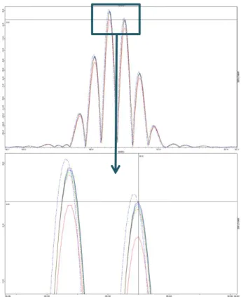
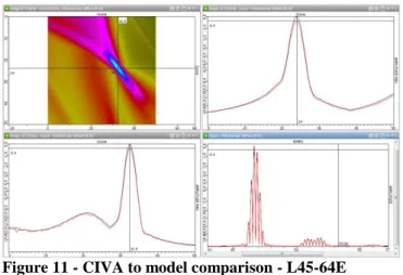
Figure 11 - CIVA to model comparison - L45-64E
In red, CIVA, in black the new model.
Upper left: Simulated image - Upper right: Graph of the vertical maxima Lower left: Graph of the horizontal maxima - Lower right: Maximum signal
Figure 12 - CIVA to model comparison - L45-64EP
In red, CIVA, in black the new model.
Upper left: Simulated image - Upper right: Graph of the vertical maxima Lower left: Graph of the horizontal maxima - Lower right: Maximum signal
Figure 11 and Figure 12 highlight the focal spot measurement on the simulated image. Table 2 presents the measurement results for all the studied configurations and the relative error compared to CIVA. First, it is noteworthy that this model slightly overestimates the amplitude obtained by CIVA 11.0; however, in all cases, the discrepancy is less than 0.4 dB (~5%) and remains below the requirements for passing benchmarks against experimental results. Moreover, the focal spot is of the same dimension with both tools, the relative observed error is inferior to 2%. Lastly, results indicate the absence of temporal shift between CIVA and this model (as observed on previous Figures). Thus, those results validate this new UT field computation model in terms of amplitude, beam shape and time of flight.
IV. Model benchmarking
The two implementations (GPU and GPP) have been benchmarked on high-end hardware to aim at a fair evaluation of performances.
1. GPP benchmarking
Two GPP configurations have been studied:
- GPP1 - 2x GPP Intel Xeon [email protected] + 24GB of RAM : which disposes of 2x6 hardware core (2x12 logical cores with HyperThreading);
- GPP2 2x GPP Intel Xeon [email protected] + 24GB of RAM : which disposes of 2x8 hardware core (2x16 logical cores with HyperThreading);
Over those two GPP configurations, several tools have been studied through two versions of the implementation: one using a legacy FFT implementation compiled with Microsoft Visual C++ 20101 versus one using the Intel® MKL built with the ICC compiler2.
In this paragraph, the study will focus successively, on the scaling capability of this implementation, then on the impact of the hyperthreading before focusing on the impact of the Intel tools.
Figure 13 – Scaling of the application
In those graphs, execution of a L0_64E configuration, with 200x200 field point are studied on GPP1 and GPP2 (16threads). The scaling is then computed by comparing the monothread execution time to the actual time with N threads. This scaling is then presented in the following graph, normalized by the number of threads (a theorical perfect scaling is 1). Compiler : MSVC.
1
MSVC Version 16.00.40219.01 with Visual Studio 2010 SP1
2
Intel(R) C++ Intel(R) 64 Compiler XE, Version 14.0.0.103 Build 20130728
Single precision floating point L0-32E L0-64E L0-64EP L45-32E L45-64E L45-64EP 1 thread MSVC + Legacy FFT 2610 ms x 1,00 5440 ms x 1,00 3512 ms x 1,00 5578 ms x 1,00 7471 ms x 1,00 7541 ms x 1,00 ICC + iMKL 1049 ms x 2,49 2160 ms x 2,52 1818 ms x 1,93 2255 ms x 2,47 3804 ms x 1,96 3913 ms x 1,93 2x6 threads MSVC + Legacy FFT 251 ms x 1,00 514 ms x 1,00 321 ms x 1,00 527 ms x 1,00 691 ms x 1,00 697 ms x 1,00 ICC + iMKL 111 ms x 2,26 216 ms x 2,38 174 ms x 1,84 228 ms x 2,31 360 ms x 1,92 366 ms x 1,90
Table 3 - GPP Results - speedup for ICC & MKL – hardware GPP1 - 2x Xeon 5590 6 cores without HT
The first benchmark aims at measuring the scaling of the application as illustrated in Figure 13. It is noteworthy that the attained speedup is decreasing as the number of threads increases; however the overall speedup is 87% of the maximum. This shows clearly that the elementary impulse response contributions benefits from a great speedup, with a sustained one over 95%. However, the scaling of the signal formation drop to 85% as the number of threads increases. Noteworthy information is that the scaling is independent of the hardware configuration. A similar study has been realized over hyper threading. For references, the sustained speedup with 24 threads on GPP1 was 11.95 with, 13.67 for elementary contribution computation and 11.35 for the signal computation whereas those speedups are, respectively, 10.77 (+1.18x); 11.48 (+2.19x) and 10.50 (+0.85x). Hyper threading thus offers a lower benefit to the signal summation than to the rest of the implementation. Figure 14 highlights this tendency, where it is observable that the speedup is quite similar for the different configurations.
Figure 14 - Scaling on GPP1 for each configuration
Another noteworthy result from Table 3 is that the usage of MKL and ICC provide a non-negligible speed up from 1.93 to 2.52 in monothread execution. However, this speed up is down from x1.84 to x2.38 once executed over 2x6 threads on the overall execution time: some computations, like the construction of the MKL FFT plan, do not benefit as much of parallel execution.
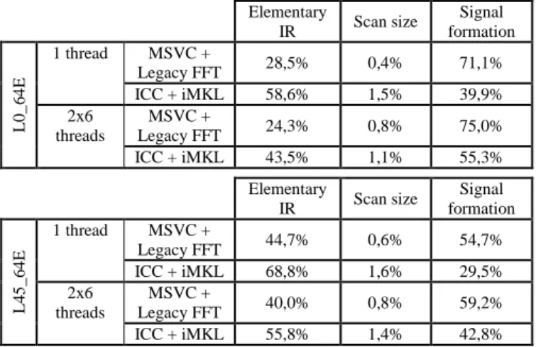
Table 4 presents the time repartition over executing GPP implementations on L0_64E and L45_64E. This confirms that the MKL execution benefit greatly to the impulse
response signal manipulations; however the other
computations (generating elementarily impulse response, and signal size determination) do not benefits as much from the MKL as their overall proportions increase.
Elementary IR Scan size Signal formation L0 _ 6 4 E 1 thread MSVC + Legacy FFT 28,5% 0,4% 71,1% ICC + iMKL 58,6% 1,5% 39,9% 2x6 threads MSVC + Legacy FFT 24,3% 0,8% 75,0% ICC + iMKL 43,5% 1,1% 55,3% Elementary IR Scan size Signal formation L4 5 _ 6 4 E 1 thread MSVC + Legacy FFT 44,7% 0,6% 54,7% ICC + iMKL 68,8% 1,6% 29,5% 2x6 threads MSVC + Legacy FFT 40,0% 0,8% 59,2% ICC + iMKL 55,8% 1,4% 42,8%
Table 4 - Execution time repartition on GPP1
2. GPU benchmarking
On the GPU side, four different GPU have been studied. Those GPU are of the same architecture, NVIDIA codename Fermi, which diverge only by their intrinsic characteristics (number of CUDA cores, core frequency, and memory bandwidth). The GPU are listed in Table 5 for reference. In this section will be discussed the predictability of performances over a whole range of GPU for a single configuration ; then a more in depth study will focus on the impact of atomic operations over the performances.
Chip # of SM # of cores Core frequency Memory bandwidth GTX 480 GF100 15 480 1215Mhz 177.4GB/s Tesla C2070 GF100 14 448 1150Mhz 144GB/s GTX 570 GF110 15 480 1464Mhz 152 GB/s GTX 580 GF110 16 512 1554Mhz 192.4 GB/s
Table 5 - GPUs studied
As the objective of this model is the UT field simulation resulting, the computed product is an image of such small size (100x100 float=40kb) that its transfer time is negligible before the computation time. Hence, in this section, the presented computation time do not take into account data transfer to and from the host.
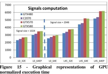
Figure 15 - Graphical representations of GPU normalized execution time
This graph presents signal computation time normalized relatively to the signal size
In Figure 15, those results are presented in graphs one for each step. It has to be noted that the normalized performances of the streaming multiprocessors of those GPUs are roughly the same for a given frequency and for a given memory bus. More precisely, this statement works best with GPU relying on the same chipset (GTX 580 and 570; GTX 480 and Tesla C2070). The redesign of the GF100 by NVidia into GF110 not only increased thermal efficiency but also benefited lightly to GPGPU performances. Moreover, this behavior is a first step toward performances prediction for a given field simulation of this algorithm on different GPU using those chipset (for those simulations), based on the measured performances for this partial set of GPUs.
Another key element to the performance is the required signal size. Experiments L0_64E and the L45 ones require a larger signal size than others to accommodate with the summation of elementary displacement over the signals (signals of size 2048 float elements versus 1024 for simpler configurations). This impacts performance at two levels: first, the size directly impacts the application of cuFFT on larger chunks of memory; secondly a wider temporal span of information means a higher collision rate when operating atomic addition to sum contributions over the signal.
To establish the impact of atomic memory operations over the simulation, Figure 16 presents the normalized execution time on a GTX 580 and a C2070 with and without them. It shows clearly that atomic addition can slow down performances, increasing execution time up to a factor 2, when memory collisions go bad. It is remarkable that performances become quasi linear to the signal size in their absence which reveals their preponderance over the rest of the computations.
Figure 16 – GPU normalized time with and without atomic operations (C2070 and GTX580 only)
This graph presents signal computation time normalized relatively to the signal size
4. Raw performances summary
In both previous sections, benchmarks have been dedicated over a single architecture. To summarize this study, Table 6 presents the best performances of this simulation over all the configurations for GPP and GPU with a temporal point of view. It appears that GPP performs better than GPU on the whole set of configurations. For modest sized problems, simulation is able to reach 10 images per second on GPP whereas GPU cap at 6.2 images per second (L0_32E).
L0_32E L0_64E L0_64EP L45_32E L45_64E L45_64EP CIVA 11.0 1,9E+04 ms 4,1E+04 ms 4,7E+04 ms 6,1E+04 ms 1,4E+05 ms 2,2E+05 ms GTX 580 161ms 350ms 216ms 437ms 610ms 719ms 6,2fps 2,9fps 4,6fps 2,3fps 1,6fps 1,4fps 2xXeon +HT 96ms 195ms 144ms 200ms 321ms 308ms 10,4fps 5,1fps 6,9fps 5,0fps 3,1fps 3,2fps
Table 6 - Performances summary (GPU and GPP)
GPU using GTX 580;
GPP using GPP1 - 2x GPP Intel Xeon 5590 with Intel ICC and MKL;
To conclude this benchmark, both implementations still require at least a speedup over an order of magnitude to reach full interactive performances. On GPP, one strategy may be to adopt a full SIMD implementation of compute-heavy sections. On GPU, work will focus on the summation of small contributions over temporal signals to reduce the influence of atomic operation.
V. Conclusion
This paper presented a new model for UT field computation, aimed at providing regularity toward massively parallel architectures. This model suffers from a lack of genericity. Indeed, the regular ray path computation requires analytical modeling of surfaces, this model is limited to canonical components, made of homogeneous and isotropic material and to direct and half-skip mode. This model has been validated, by comparison with the CIVA 11.0 software, against typical configurations and provides accurate field simulation. This new model has been implemented on both
0 1000 2000 3000 4000 5000 6000 7000
L0_32E L0_64EP L0_64E L45_32E L45_64E L45_64EP
Signals computation GTX480 C2070 GTX570 GTX580 Signal size = 1024 Signal size = 2048
GPP and GPU, and the preliminary conclusions come as follows.
On the GPP, the implementation performances scales with the number of threads, however, this scaling is hindered on the signal formation step. By using Intel MKL and the Intel compiler, it is possible to increase the overall performances of the application by a factor 2. However, as the MKL is used for speeding up signal processing, this speedup is not shared by the other parts of the computation.
Concerning GPUs, performances of a given computation are predictable on different GPU relying on the same chipset once this configuration is benchmarked on a single hardware. Benchmarks highlight the cost of atomic operations, which can be much slower than standard memory operations when there are a lot of collisions. Those operations amount to performances up to twice slower than standard memory operations.
Overall performances reach, for GPU, 6.2fps on modest sized configuration and can be as slow as 1.4fps on heavyweight one; whereas the GPP reaches a frame rate of 10.4fps and 3.1fps respectively. This performance is already good but still requires at least, an order of magnitude to attain interactive field simulation.
Finally, multiple improvements can be sought to speed up each parallel implementation. For example, the use of SIMD instruction on the GPP to benefit from its fine grained parallel abilities (especially on the non signal-processing steps i.e. pencil computations). Besides, by reducing the number of atomic operations in the GPU implementation, performances can improve drastically on signal summation. Work is also in progress to provide an extensive benchmark framework, aimed to provide an auto-tuning algorithm, adapting its parameters to the class of configuration and to the hardware architecture.
Those implementations are the first step toward a fast UT simulation integrated within the CIVA 12 software.
VI. References
1. M. Molero, and U. Iturraràn-Viveros, Accelerating numerical
modeling of wave propagation through 2-D anisotropic materials using OpenCL, 2013, vol. 53, pp. 815 – 822. 2. D. Romero-Laorden, O. Martínez-Graullera, C. J. Martín, M.
Pérez, and L. G. Ullate, Field modeling acceleration on
ultrasonic systems using graphic hardware, 2011, vol. 182, pp.
590–599.
3. N. Gengembre, Pencil method for ultrasonic beam
computation. In Proc. of the 5th World Congress on
Ultrasonics, pages 1533–1536 (2003).
4. J Lambert et al., Performance evaluation of total focusing method on GPP and GPU. In Proc. of the DASIP conference, pages 265-272 (2012)