HAL Id: hal-01319131
https://hal.inria.fr/hal-01319131
Submitted on 20 May 2016
HAL is a multi-disciplinary open access
archive for the deposit and dissemination of
sci-entific research documents, whether they are
pub-lished or not. The documents may come from
teaching and research institutions in France or
abroad, or from public or private research centers.
L’archive ouverte pluridisciplinaire HAL, est
destinée au dépôt et à la diffusion de documents
scientifiques de niveau recherche, publiés ou non,
émanant des établissements d’enseignement et de
recherche français ou étrangers, des laboratoires
publics ou privés.
Comparing functional connectivity based predictive
models across datasets
Kamalaker Dadi, Alexandre Abraham, Mehdi Rahim, Bertrand Thirion, Gaël
Varoquaux
To cite this version:
Kamalaker Dadi, Alexandre Abraham, Mehdi Rahim, Bertrand Thirion, Gaël Varoquaux.
Compar-ing functional connectivity based predictive models across datasets. PRNI 2016: 6th International
Workshop on Pattern Recognition in Neuroimaging, Jun 2016, Trento, Italy. �hal-01319131�
Comparing functional connectivity based predictive
models across datasets
Kamalaker DADI
∗†, Alexandre ABRAHAM
∗†, Mehdi RAHIM
∗†, Bertrand THIRION
∗†, Ga¨el VAROQUAUX
∗†∗Parietal Team, INRIA, Paris-Saclay University, France.
†CEA, DSV, I2BM, Neurospin Center, Paris-Saclay University, 91191, Gif-sur-Yvette, France.
Email: [email protected]
Abstract—Resting-state functional Magnetic Resonance Imag-ing (rs-fMRI) holds the promise of easy-to-acquire and wide-spectrum biomarkers. However, there are few predictive-modeling studies on resting state, and processing pipelines all vary. Here, we systematically study resting state functional-connectivity (FC)-based prediction across three different cohorts. Analysis pipelines consist of four steps: Delineation of brain regions of interest (ROIs), ROI-level rs-fMRI time series signal extraction, FC estimation and linear model classification analysis of FC features. For each step, we explore various methodological choices: ROI set selection, FC metrics, and linear classifiers to compare and evaluate the dominant strategies for the sake of prediction accuracy. We achieve good prediction results on the three different targets. With regard to pipeline selection, we obtain consistent results in two pipeline steps –FC metrics and linear classifiers– that are vital in the diagnosis of rs-fMRI based disease biomarkers. Regarding brain ROIs selection, we observe that the effects of different diseases are best characterized by different strategies: Schizophrenia discrimination is best performed in dataset-specific ROIs, which is not clearly the case for other pathologies. Overall, we outline some dominant strategies, in spite of the specificity of each brain disease in term of FC pattern disruption.
Index Terms—Functional connectivity, connectome, resting-state, predictive model
I. INTRODUCTION
Resting-state functional magnetic resonance imaging (rs-fMRI) is a non-invasive and easy-to-acquire modality. It pro-vides measurements of brain function that can characterize a wide range of phenotypic traits [1]. Indeed, it has been used to discriminate neurological diseases and psychiatric disorders [2], but also to predict different mental states [3] and has even been used as a unique fingerprint for each individual [4]. FC is also a potential biomarker for early diagnosis and disease progression. For this, analysis pipelines are used to estimate the connectome from rs-fMRI, and then to build a classification model that predicts the clinical group from the resulting FC estimates. Such a pipeline has been introduced in [5], where sparse FC network estimates are used to classify subjects with major depression disorder from healthy subjects. A fully-automated pipeline has been proposed recently to high-light autism biomarkers [6] from large and multi-site autism datasets. The setting of an effective analysis pipeline requires to tune many parameters, either in the feature extraction or in the classification, in order to have the best possible prediction. Setting pipeline parameters is not straightforward and typically results into huge variations across datasets. In addition, it is
not known to what extent an optimal pipeline setting for a given dataset can be reused for another dataset, and if there are some dominant strategies.
We study in this paper whether parameters can be reliably selected to answer diverse clinical questions based on FC measurements obtained from three different datasets. Our aim is to overcome the heterogeneity in the data, related to image quality or to the disease under study, by outlining consistent effects across large resting state FC datasets related to various psychiatric disorders. We compare the impact of each pipeline step on the prediction accuracy on these datasets that target different disease characterizations. This gives us a better understanding on what choices should be made to establish accurate diagnosis models of neuropsychiatric disorders.
II. METHODS: CONNECTIVITY ANALYSIS PIPELINE
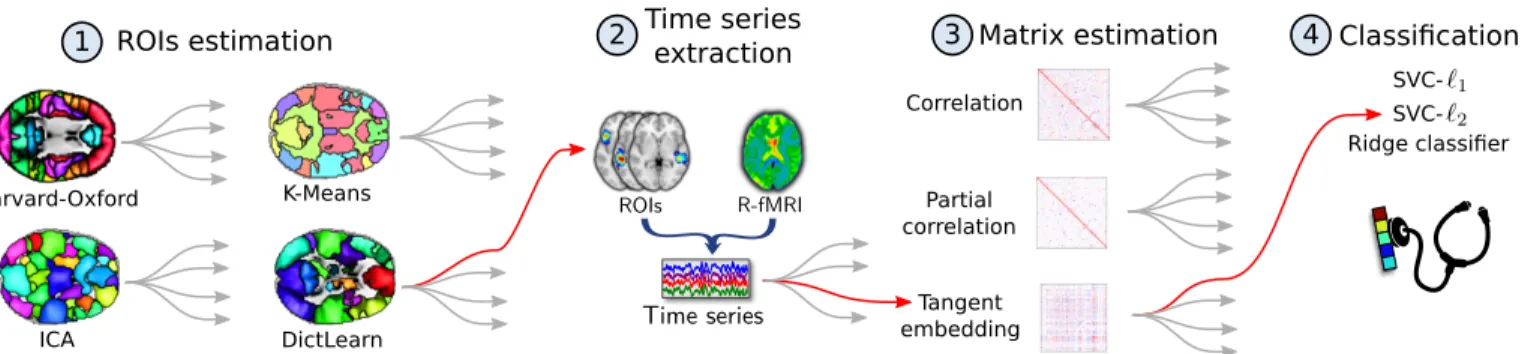
Fig.1 depicts our prediction pipeline. It consists of four steps: i) Definition of brain regions of interest (ROIs), ii) Extraction of the time series associated with these ROIs, iii) Estimation of FC metrics from these time series, iv) Connectivity-based classification of the phenotypic target. A. ROIs definition
The first step of the pipeline aims at reducing the dimension-ality of the problem by aggregating voxels into ROIs forming an atlas. We use two kinds of approaches: i) reference atlases previously defined on other structural or functional datasets, and ii) atlases directly learned from the data. The question underlying atlas selection is whether different brain disorders lead to a consistent choice, and whether genericity should be preferred to adaptive strategies. Because we want to study the connectivity between spatially contiguous ROIs and not between brain networks, we use a Random Walker approach to segment ROIs in the models composed of networks (i. e. all except AAL and Ward) as proposed in [7]. During this procedure, we remove spurious regions (size < 1900mm3).
An example of the atlases obtained through dictionary learning is presented in Fig.2.
Predefined atlases: We select two reference atlases learned on structural MRI and one learned on functional MRI. Automated Anatomical Labeling (AAL) [8] is an anatomical atlas of 116 regions obtained on a single subject. Harvard-Oxford (HO) [9] is a probabilistic cortical segmentation of 48 bi-hemispheric regions performed on 40 subjects. We extract
ROIs estimation
Harvard-Oxford
ICA DictLearn K-Means
Time series
extraction Matrix estimation
Correlation Partial correlation Tangent embedding Classification Ridge classifier SVC-R-fMRI ROIs Time series 4 1 2 3
Fig. 1: Resting state functional connectivity prediction pipeline. Step 1 defines brain ROIs using predefined reference atlases or data-driven methods. Step 2 extracts time series from each ROI. Step 3 estimates pairwise functional connectivity between ROIs, using correlation, partial correlation or tangent space embedding. In step 4, a classification model is built to predict groups with two linear classifiers, SVC (`1 or `2 penalization) and ridge regression (`2 penalization).
90 ROIs to study spatially contiguous regions. Bootstrap Analysis of Stable Clusters (BASC) [10] is a multi scale functional atlas estimated using K-Means clustering on rs-fMRI dataset that consists of 43 healthy individuals. We use the 64 network atlas, yielding 97 ROIs.
Regions extracted from the data: We use four data exploratory methods to segment ROIs from fMRI: i) two clustering approaches: K-Means and hierarchical agglomer-ative clustering using Ward’s algorithm [11], and ii) two data decomposition methods, namely multi-subject Indepen-dent Component Analysis (ICA) [12] and Online Dictionary Learning (DictLearn) [13].
Fig. 2: Functional ROIs obtained using Dictionary Learn-ing on ADNI (left), COBRE (middle), ACPI (right) datasets. After region extraction, the ADNI, COBRE and ACPI atlases comprise 115, 105 and 133 ROIs respectively Each region is shown with different color.
B. Time-series signals extraction
In this step, we extract a representative time-series for each ROI in each subject. For atlases composed of non-overlapping ROIs, we simply compute the average of the fMRI time series signals over all voxels within that specific region. For fuzzy overlapping ROIs, such as the components extracted by ICA and DictLearn, we use least squares regression method to compute signals over several overlapping ROIs. The signal of each region is then normalized, detrended and bandpass-filtered between 0.01 and 0.1 Hz.
C. Functional connectivity estimation
FC is defined as the covariance between signals from brain ROIs. Given that the time-series are too short to estimate the true covariance matrix, we use a regularized shrinkage estimation. We choose the Ledoit-Wolf estimator [14] because it is parameter free and an efficient implementation is available in the scikit-learn library [15]. With this covariance structure, we study three different connectivity measures: correlation, partial correlation (from the inverse covariance matrix) [16] and the tangent embedding parametrization of the covariance matrix [17].
D. Connectivity-based classification
In the final step of our pipeline, we predict a binary phenotypic status from FC. We extract the lower triangular part of the connectivity matrix as a set of features for the prediction task [3]. We consider the Linear Support Vector Classifier (SVC) with `1 and `2 regularization and the Ridge
Classifier with `2 penalization.
III. EXPERIMENTS ON MULTIPLE DATASETS
A. Datasets
We experiment our classification pipeline on three rs-fMRI datasets. Models built from connectivity features pre-dict various clinical outcomes (degenerative and neuro-psychiatric disorders, drug abuse impact). The first dataset is from the Center for Biomedical Research Excellence (CO-BRE) [18]. The pipeline predicts the schizophrenia diagnosis of the subjects. The second dataset is the Alzheimer’s Dis-ease Neuroimaging Initiative (ADNI) [19]. We discriminate Alzheimer’s Disease (AD) from Mild Cognitive Impairment (MCI) group. The third dataset is the Addiction Connectome Preprocessed Initiative (ACPI)1, where we discriminate
Mar-ijuana consumers versus control subjects.
All rs-fMRI acquisitions are preprocessed using standard steps that include motion correction, co-registration to T1-MRI, normalization to the MNI template, Gaussian spatial
smoothing (FWHM=5mm), and temporal detrending. All sub-jects were visually inspected and excluded from the analysis if they had severe scanner artifacts or head movements with amplitude larger than 2mm. The total number of subjects then selected from COBRE, ADNI, ACPI are 81, 137, 126 respectively (table I).
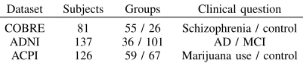
TABLE I: Description of the three datasets used.
Dataset Subjects Groups Clinical question COBRE 81 55 / 26 Schizophrenia / control
ADNI 137 36 / 101 AD / MCI ACPI 126 59 / 67 Marijuana use / control
B. Experiment design
Classification setting: Our approach is a binary classifica-tion to predict the phenotype status. We set a cross-validaclassifica-tion framework by randomly shuffling and splitting populations over 100 runs into 75% for training the classifier and testing on the remaining 25%. In each fold, we preserve the percentage of samples between groups. For each split, we measure the Area Under the Curve (AUC) from the Receiver Operating Characteristics (ROC) curve. The final prediction scores (more than 10k scores: 63 types of pipelines × 3 datasets × 100 splits) obtained across all datasets are used in a post-hoc statistical analysis to evaluate the importance of each step in our prediction model.
Post-hoc analysis setting: We use a full factorial Analysis of Variance (ANOVA), with three major factors of importance: the atlas (AAL, Harvard Oxford, BASC, K-Means, Ward, ICA, DictLearn), the connectivity estimator (correlation, partial cor-relation, tangent space), and the classifier (svc `1, svc `2,
ridge). For each factor, we compare the significance of each choice and its effect (positive or negative) on the classification performance.
Software used: We use SPM8 for preprocessing, Nilearn [20] for feature extraction, Scikit-learn [15] for classification, and Statsmodels [21] for post-hoc comparisons.
IV. RESULTS AND DISCUSSION
We study the impact of each pipeline step on the model accuracy, and its consistency over diverse clinical questions.
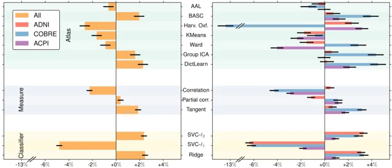
To measure the impact of the different options on the predic-tion scores relative to the mean predicpredic-tion, we perform a full-factorial analysis of variance (ANOVA) on prediction scores. In a linear model, each step of the pipeline is considered as a categorical variable and its contribution is given by its coefficient. Fig.3 gives the results on each dataset (on the right) and a summary analysis on the pooled data (on the left). Error bars give the 95% confidence interval.
Across all datasets, `2-penalized classifiers clearly
outper-form `1penalization. In addition, using the tangent embedding
as a connectivity measure gives a consistent improvement over correlations and partial correlation.
With regards to functional regions, the trend is not as clear. The analysis across datasets (Fig.3right) reveals that the most
TABLE II: Comparison of the atlas impact on prediction accuracy. Reported values are the mean and standard deviation of AUC over 100 iterations. Best predictions are in bold.
COBRE ADNI ACPI AAL .79 ± .09 .66 ± .09 .58 ± .08 BASC .83 ± .08 .67 ± .09 .59 ± .08 DictLearn .83 ± .08 .66 ± .07 .62 ± .07 HO .62 ± .11 .68 ± .09 .62 ± .09 ICA .83 ± .08 .68 ± .09 .56 ± .08 K-Means .79 ± .08 .64 ± .09 .56 ± .08 Ward .83 ± .08 .64 ± .08 .53 ± .09
effective atlases are those learned on functional data (BASC, ICA, Dictionary Learning).
However, further dataset-specific analyses (Fig.3left) reveal some discrepancies across the datasets. One of the most striking observation is the inability of Harvard-Oxford to discriminate typical controls and schizophrenic patients (CO-BRE dataset). As an anatomical atlas, it lacks some crucial functional regions.
TableIIgives the accuracy and best strategy for selection of brain ROIs per dataset. Conclusions vary. Schizophrenic sub-jects (COBRE) are most easily discriminated with functional-data-driven ROIs, whereas no such effect is observed in the other datasets (ADNI or ACPI). Note however that prediction accuracy is lower in these datasets.
Brain atlases learned with BASC, ICA, or DictLearn con-sistently obtain high scores across different clinical questions and datasets. On the opposite AAL, K-Means, Ward, Harvard-Oxford have very uneven performance levels across target variables and datasets. We stipulate that the benefits of BASC, ICA, and DictLearn are not only that they use functional information to capture regions, but also that they rely on a probabilistic or soft-assignment model. Indeed BASC is obtained via bootstrapped clustering, and ICA or DictLearn are linear decomposition models. Interestingly, BASC was extracted from another dataset not included in our study, yet it achieves relatively good performance. This suggests that some aspects of a good set of regions carry over from one cohort to another. Indeed, the DictLearn atlases extracted on our three cohorts show high similarities with regards to the large networks that they outlined (see Fig.2).
V. CONCLUSION ANDFUTUREWORK
In this paper, we presented a functional connectivity-based analysis pipeline to predict diverse behavioral targets from rs-fMRI data. Our contribution lies in the systematic exploration of commonly used models for each step of the pipeline and in the study of the impact of these steps on the prediction. We show guidelines for classifier selection and covariance estimation: Rely on `2 classifiers; Use the tangent space
embedding of the covariance matrix. The brain atlas selection in the pipeline does not give a clear trend. Overall, functionally driven regions with Dictionary Learning, group ICA or BASC atlas perform well across datasets.
Further work calls for exploring more datasets to confirm trends on best-performing methods, as well as detailed
investi--13% -6% -4% -2% +0% +2% +4% Atlas Measure Classifier All ADNI COBRE ACPI -13% -6% -4% -2% +0% +2% +4% AAL BASC Harv. Oxf. KMeans Ward Group ICA DictLearn Correlation Partial corr. Tangent SVC-`2 SVC-`1 Ridge
Fig. 3: Post-hoc comparisons between pipeline choices on the rs-fMRI datasets. Single factor analysis (right) with each dataset (ADNI, COBRE, ACPI) and on pooled data (left). We observe that: (i) Tangent embedding performs better than correlation or partial correlation in all datasets. (ii) `2 regularized classifiers SVC and Ridge are more accurate than SVC-`1
classifier. (iii) With regards to brain atlases, decomposition methods (ICA, DictLearn) are generally the best choices, though with striking cross-datasets differences.
gation of functional-connectivity differences across groups to give insights on disease biomarkers.
ACKNOWLEDGMENT
This work is jointly supported by the NiConnect project (ANR-11-BINF-0004 NiConnect) and CATI project.
REFERENCES
[1] S. M. Smith, T. E. Nichols, D. Vidaurre et al., “A positive-negative mode of population covariation links brain connectivity, demographics and behavior,” Nature neuroscience, vol. 18, 2015.
[2] M. Greicius, “Resting-state functional connectivity in neuropsychiatric disorders,” Current opinion in neurology, vol. 21, p. 424, 2008. [3] J. Richiardi, H. Eryilmaz, S. Schwartz, P. Vuilleumier, and D. Van
De Ville, “Decoding brain states from fMRI connectivity graphs,” NeuroImage, 2010.
[4] E. S. Finn, X. Shen, D. Scheinost, M. D. Rosenberg, J. Huang, M. M. Chun, X. Papademetris, R. T. Constable, D. D. Lee, and H. S. Seung, “Functional connectome fingerprinting: identifying individuals using patterns of brain connectivity,” Nat Neurosci, vol. 18, 2015.
[5] M. J. Rosa, L. Portugal, T. Hahn, A. J. Fallgatter, M. I. Garrido, J. Shawe-Taylor, and J. Mourao-Miranda, “Sparse network-based models for patient classification using fmri,” NeuroImage, vol. 105, 2015. [6] A. Abraham, M. Milham, A. Di Martino, C. Craddock, D. Samaras,
B. Thirion, and G. Varoquaux, “Inter-site autism biomarkers from resting-state fMRI,” Neuroimage, in revision, 2016.
[7] A. Abraham, E. Dohmatob, B. Thirion, D. Samaras, and G. Varoquaux, “Region segmentation for sparse decompositions: better brain parcella-tions from rest fMRI,” in STMI, 2014.
[8] N. Tzourio-Mazoyer, B. Landeau, D. Papathanassiou, F. Crivello, O. Etard, N. Delcroix, B. Mazoyer, and M. Joliot, “Automated anatom-ical labeling of activations in SPM using a macroscopic anatomanatom-ical parcellation of the MNI MRI single-subject brain.” Neuroimage, 2002. [9] R. S. Desikan, F. S´egonne, Fischl et al., “An automated labeling system for subdividing the human cerebral cortex on MRI scans into gyral based regions of interest,” Neuroimage, vol. 31, p. 968, 2006.
[10] P. Bellec, P. Rosa-Neto, O. Lyttelton, H. Benali, and A. Evans, “Multi-level bootstrap analysis of stable clusters in resting-state fMRI,” Neu-roImage, vol. 51, p. 1126, 2010.
[11] B. Thirion, G. Varoquaux, E. Dohmatob, and J.-B. Poline, “Which fmri clustering gives good brain parcellations?” Frontiers in neuroscience, vol. 8, 2014.
[12] G. Varoquaux, S. Sadaghiani, P. Pinel, A. Kleinschmidt, J. B. Poline, and B. Thirion, “A group model for stable multi-subject ICA on fMRI datasets,” NeuroImage, vol. 51, p. 288, 2010.
[13] J. Mairal, F. Bach, J. Ponce, and G. Sapiro, “Online dictionary learning for sparse coding,” ICML, 2009.
[14] O. Ledoit and M. Wolf, “A well-conditioned estimator for large-dimensional covariance matrices,” J. Multivar. Anal., 2004.
[15] F. Pedregosa, G. Varoquaux, A. Gramfort, V. Michel et al., “Scikit-learn: Machine learning in Python,” Journal of Machine Learning Research, 2011.
[16] G. Varoquaux and C. Craddock, “Learning and comparing functional connectomes across subjects,” NeuroImage, vol. 80, p. 405, 2013. [17] G. Varoquaux, F. Baronnet, A. Kleinschmidt, P. Fillard, and B. Thirion,
“Detection of brain functional-connectivity difference in post-stroke patients using group-level covariance modeling,” in MICCAI, 2010. [18] V. D. Calhoun, J. Sui, K. Kiehl, J. Turner, E. Allen, and G. Pearlson,
“Exploring the psychosis functional connectome: aberrant intrinsic net-works in schizophrenia and bipolar disorder,” Frontiers in psychiatry, 2011.
[19] S. G. Mueller, M. W. Weiner, L. J. Thal, R. C. Petersen, C. Jack, W. Jagust, J. Q. Trojanowski, A. W. Toga, and L. Beckett, “The alzheimer’s disease neuroimaging initiative,” Neuroimaging Clinics of North America, vol. 15, no. 4, pp. 869–877, 2005.
[20] A. Abraham, F. Pedregosa, M. Eickenberg, P. Gervais, A. Mueller, J. Kossaifi, A. Gramfort, B. Thirion, and G. Varoquaux, “Machine learn-ing for neuroimaglearn-ing with scikit-learn,” Frontiers in neuroinformatics, 2014.
[21] S. Seabold and J. Perktold, “Statsmodels: Econometric and statistical modeling with python,” in Proceedings of the 9th Python in Science Conference, 2010.