Control of spacecraft in proximity orbits

(1)

Control of Spacecraft in Proximity Orbits

by

Louis Scott Breger

Bachelor of Science Aeronautics and Astronautics

Massachusetts Institute of Technology, 2002

Master of Science Aeronautics and Astronautics

Massachusetts Institute of Technology, 2004

Submitted to the Department of Aeronautics and Astronautics

in partial fulfillment of the requirements for the degree of

Doctor of Philosophy

at the

MASSACHUSETTS INSTITUTE OF TECHNOLOGY

June 2007

@

Louis Scott Breger, MMVII. All rights reserved.

The author hereby grants to MIT permission to reproduce and

distribute publicly paper and electronic copies of this thesis document

in whole or in part.

A u th o r ...

. ...

...

Department of Aeronautics and Astronautics

June 8, 2007

Certified by...

...

Jonathan P. How

Associate Professor of Aeronautics and Astronautics

Thesis Supervisor A ccepted by ... . . w .... . . . . . . . .

\p

bJaime

Peraire

Professor of Aeronautics and Astronautics

MASSACHUSETTS INSTITUTE

Chair, Committee on

Graduate

Students

OF TECHNOLOGYChiCmiteoGrdaeSuns

JUL 1

12007-

ARCHN\ES

(2)

(3)

Control of Spacecraft in Proximity Orbits

by

Louis Scott Breger

Author .... ... .:...

Department of Aeronautics and Astronautics

June 8, 2007

Accepted by ...

Jonathan How

Associate Professor of Aeronautics and Astronautics

Thesis Supervisor

Accepted by...

Accepted by ....

...

. .

.

. .. .

W .

l ri n

Kylofr Alfriend

Professor of Aerospace Engineering, Texas A&M

. . . .. . . . .

John Deyst

Associate Professor of Aeronautics and Astronautics

A ccepted by ...

Raymond Sedwick

Principal Research Scientist, Aeronautics and Astronautics

(4)

(5)

Control of Spacecraft in Proximity Orbits

by

Louis Scott Breger

Submitted to the Department of Aeronautics and Astronautics on June 8, 2007, in partial fulfillment of the

requirements for the degree of Doctor of Philosophy

Abstract

Formation flying of spacecraft and autonomous rendezvous and docking of space-craft are two missions in which satellites operate in close proximity and their relative trajectories are critically important. Both classes of missions rely on accurate dynam-ics models for fuel minimization and observance of strict constraints for preventing collisions and achieving mission objectives. This thesis presents improvements to spacecraft dynamics modeling, orbit initialization procedures, and failsafe trajectory design that improve the feasibility and chances of success for future proximity opera-tions. This includes the derivation of a new set of relative linearized orbital dynamics incorporating the effects of Earth's oblateness. These dynamics are embedded in a model predictive controller, enabling LP-based MPC formulations for large baseline formations in highly elliptic orbits. An initialization algorithm is developed that uses the new dynamics to optimize multiple objectives (drift and fuel usage minimization, geometry) over science-relevant time frames, improving previous J2-invariant

initial-ization techniques which only considered infinite-horizon secular drift. The trajectory planning algorithm is used to design spacecraft rendezvous paths that observe realistic constraints on thruster usage and approach path. The paths are fuel-optimized and further constrained to be safe (i.e., avoid collisions) in the presence of many possible system failures, an enhancement over previous guaranteed-safe rendezvous methods, which did not minimize fuel use. The fuel costs of imposing safety as a constraint on trajectory design are determined to be low compared to standard approaches and a stochastic analysis demonstrates that both active and passive forms of the safe rendezvous algorithm substantially decrease the likelihood of system failures result-ing in collisions. The effectiveness of the new controller/dynamics combination is demonstrated in high fidelity multi-week simulations. An optimized safe rendezvous trajectory was demonstrated on a hardware testbed aboard the International Space Station.

Thesis Supervisor: Jonathan P. How

(6)

(7)

Acknowledgments

I would like to thank everyone who has assisted me in my academic career. My par-ents and sister have supported me in every way and taught me the most important principles of graduate work long before my arrival at MIT. A complete list of every-one who's had a hand in this thesis would include my teachers through MIT, high school, and even earlier. I've been fortunate to have had access to an exceptional education and many good people to steer me along the way. In particular, I'd like to thank my first control systems instructors: Winston Markey, John Deyst, and Emilio Frazzoli. The semester-long introductory class they taught in automatic control in the Fall of 2000 changed the course of my life and I am grateful for having had the opportunity to study under them. Likewise, Lorraine Fesq helped me immeasurably in my quest to enter graduate school and find work afterward by providing me with many of my most treasured job experiences. Terry Alfriend's generous donations of time, expertise, and renowned intuition have enabled much of this research. The SPHERES team (in particular, Simon Nolet, Nick Hoff, and Chris Mandy) deserve many thanks for the time and effort they put into helping me get experiments working on their hardware and on ISS. My fellow labmates (notably Yoshiaki Kuwata, Arthur Richards, and Luca Bertuccelli) have always been around to bounce ideas off, study with, and even fly airplanes alongside; their companionship will be greatly missed. Kathryn Fischer's help navigating the administrative side of MIT has been indispens-able. Finally, Jonathan How, who has been my graduate and research advisor for the past five years, has taught me far far more than I ever thought I had to learn. Jon's patience, wisdom, funding, and humor were necessary conditions for producing the contributions that follow.

This thesis is dedicated to my parents, for whom the term acknowledgement seems inadequate. Their encouragement and example are my principal inspirations.

(8)

(9)

List of Figures

2-1 Effect of Orbital Element Perturbations on the ABtrue Matrix for a

LEO O rbit . . . . 40

2-2 Effect of Orbital Element Perturbations on the ABtrue Matrix for a

H EO O rbit . . . . 40

2-3 Difference between integrated and approximated P for different dis-cretization times using the LEO orbit in Eq. (2.14) . . . . 49 2-4 Difference between integrated and approximated F for different

dis-cretization times using the HEO orbit in Eq. (2.16). . . . . 50 2-5 Example of a plan generated to MPC with J2-modified GVEs (lines

indicate relative state error) . . . . 52 2-6 Error in open-loop trajectory following using the HEO orbit

exam-ple. Lines indicate the difference between planned and implemented trajectories in a fully nonlinear simulation. . . . . 54

2-7 Forming and maintaining a 1000 km (at apogee) tetrahedron

forma-tion in a highly eccentric orbit (e ~ 0.8) in the presence of J2 . . . . 62

2-8 Forming and maintaining a 1000 km (at apogee) tetrahedron

forma-tion in a highly eccentric orbit (e ~ 0.8) in the presence of J2 . . . . 63

3-1 Illustration of Initialization Approach . . . . 68 3-2 Expected drift and fuel cost of a range of optimized initial conditions

in a LEO orbit . . . . 69 3-3 Expected drift and geometry cost of a range of optimized initial

(14)

3-4 Expected drift due to differential J2 effects and fuel cost of a range of

optimized initial conditions in a HEO orbit. . . . . 73 3-5 Expected drift due to differential J2 effects and geometry cost of a

range of optimized initial conditions in a HEO orbit. . . . . 73 3-6 Relative satellite separations for a vehicle initialized using analytic

invariance and a vehicle using optimized invariance. Trajectories gen-erated using realistic nonlinear simulation including the effects J2. . 74

3-7 Relative satellite separations for a vehicle initialized using analytic in-variance and a vehicle using optimized inin-variance. Trajectories gener-ated using a nonlinear simulation that did not incorporate the effects

J2. . . . . . . .. . . 74

4-1 Concept for MELCO formation flying mission [113] . . . . 78

4-2 Summary of Station-keeping Results from Table 4.1 . . . . 84 4-3 Simulation #1: Stationkeeping in a passive aperture formation (50 m) 87 4-4 Simulation #1: Stationkeeping in a passive aperture formation (500

m ) . . . . 88

4-5 Simulation #1: Stationkeeping in a passive aperture formation (5000

m) .. ... ... ... 89

4-6 Simulation #2: Stationkeeping in a passive aperture formation (50 m) 90 4-7 Simulation #2: Stationkeeping in a passive aperture formation (500

m ) . . . . 9 1

4-8 Simulation #2: Stationkeeping in a passive aperture formation (5000

m ) . . . . 92

4-9 Simulation #3: Stationkeeping in a passive aperture formation (50 m) 93 4-10 Simulation #3: Stationkeeping in a passive aperture formation (500

m ) . . . . 94

4-11 Simulation #3: Stationkeeping in a passive aperture formation (5000

m ) . . . . 95

(15)

4-13 Simulation #4: Stationkeeping in a passive aperture formation (500 m ) . . . . 9 7

4-14 Simulation #4: Stationkeeping in a passive aperture formation (5000 m) ... .... ... . .. ... . . ... .... ... ... 98

4-15 Simulation #5: Stationkeeping in a passive aperture formation (50 m) 99 4-16 Simulation #5: Stationkeeping in a passive aperture formation (500

m) ... ... 100

4-17 Simulation #5: Stationkeeping in a passive aperture formation (5000

m) ... ... 101

4-18 Simulation #6: Stationkeeping in a passive aperture formation (50 m) 102 4-19 Simulation #6: Stationkeeping in a passive aperture formation (500

m) ... ... 103

4-20 Simulation #6: Stationkeeping in a passive aperture formation (5000 m) ... ... 104

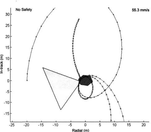
5-1 Target spacecraft and docking configuration . . . . 115 5-2 Radial/in-track view of rotating target spacecraft and docking

config-uration . . . . 115 5-3 Nominal trajectory planning with no safety: constraint violations

oc-cur for trajectory failures. . . . . 116

5-4 Trajectory planning with safety: failed trajectories deviate around the target spacecraft, preventing collision. . . . . 116 5-5 Nominal trajectory planning with no safety in the rotating case:

con-straint violations occur for trajectory failures. . . . . 120

5-6 Trajectory planning with safety in the rotating case: failed trajectories deviate around the target spacecraft, preventing collision . . . . 120

5-7 Trajectory planning with safety in the fast rotating (3/2 orbital speed) case. . . . . 12 1

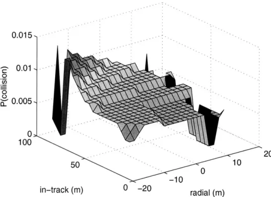
5-8 Probability of a collision occurring for a range of initial conditions with F =

0

(No safety guarantees). . . . . 124

(16)

5-9 Probability of a collision occurring for a range of initial conditions

with F = {9,... , 19} (latter half of trajectory guaranteed safe) . . . 124

5-10 Probability of collision occurring for various values of F . . . 125

5-11 Fuel required for rendezvous maneuvers for various values of F . . . 126

5-12 Amount of time required to optimize rendezvous trajectories for

var-ious values of F . . . 127

5-13 Case where end of safety horizon is followed by a collision. . . . . . 128

5-14 Use of invariance constraints guarantees infinite horizon passive col-lision avoidance and prevents failure trajectories from drifting away from the target. . . . 128

5-15 Collision avoidance for failure trajectories using convex constraints

indicated by arrows. . . . 130

5-16 Active safety demonstrated for a range of initial conditions with F =

{4,... , 19} (latter 3/4 of trajectory guaranteed safe) . . . 135

5-17 Rendezvous trajectories using active safety. . . . 139 5-18 Rendezvous trajectories using active safety with invariance constraints.

140

5-19 Rendezvous trajectories using optimized active safety. . . . . 140

5-20 Rendezvous trajectories using optimized active safety with invariance

constraints. . . . . 142

5-21 Rendezvous trajectories for using active safety optimized for two

pos-sible thruster failure directions. . . . . 142

5-22 Safe rendezvous trajectory with robustness to initial condition velocity

uncertainty . . . . 143

6-1 SPHERES Microsatellite in air carriage on flat table testbed . . . . 146

6-2 Planned safe trajectory for stationary rendezvous: x-y view. Note that trajectory z offset is zero at all times . . . . 149

6-3 SPHERES Microsatellite in air carriage on flat table testbed: Per-spective view . . . . 149

(17)

6-4 Planned safe trajectory for rotating rendezvous: x-y view. Note that trajectory z offset is zero at all times . . . . 150 6-5 Planned safe trajectory for rotating rendezvous: testbed: Perspective

view . . . . 150 6-6 SPHERES satellites docked together aboard the International Space

Station using a safe optimized rendezvous trajectory. . . . . 152 6-7 Position trajectory followed during nominal docking ISS experiment:

x-y view . . . . 153 6-8 Position time-series for z axis during nominal docking ISS experiment 153

6-9 Velocity time-series view during nominal docking ISS experiment . . 154

6-10 Velocity trajectory followed during nominal docking ISS experiment:

x-y view . . . . 154

6-11 Position trajectory followed during failed docking ISS experiment: x-y

view . . . . 155

6-12 Position time-series for z axis during failed docking ISS experiment 155

6-13 Velocity time-series view during failed docking ISS experiment . . . 156

6-14 Velocity trajectory followed during failed docking ISS experiment: x-y view . . . . 156 6-15 Position trajectory followed during failed docking flat table

experi-m ent: x-y view . . . . 158 6-16 Position time-series for z axis during failed docking flat table

experi-m ent . . . . 158

6-17 Velocity time-series view during failed docking flat table experiment 159

6-18 Velocity trajectory followed during failed docking flat table

experi-m ent: x-y view . . . . 159

7-1 Fuel Required to Maintain an In-track Formation . . . . 169 7-2 Fuel Required to Maintain a Passive Aperture Formation . . . . 169 7-3 Maneuver costs: plans created accounting for eccentricity and J2

(18)

7-4 Maneuver costs: plans created accounting for eccentricity with no J2

effects m odeled . . . 172 7-5 Maneuver costs: plans created accounting for eccentricity with no J2

effects m odeled . . . 173 7-6 Maneuver costs: plans created not accounting for eccentricity with no

(19)

List of Tables

1.1 Relative orbital dynamics indexed by regime of validity [115] . . . . 25

2.1 Average durations (in seconds) required to compute I' matrices using various m ethods . . . . 51

4.1 Fuel use results for formation flying simulations . . . . 83

5.1 Comparison of various types of safe rendezvous trajectories. . . . . . 136

(20)

(21)

Chapter 1 Introduction

Many future space missions will require autonomous proximity operations in which the knowledge and control of the relative state between space vehicles is critically important [1, 54]. Fr example, formation flying satellites operating in close prox-imity to accomplish coupled goals will require high levels of on-orbit autonomy and coordinated control [65]. Rendezvous and docking missions are also inherently con-cerned with controlling the reduction of the distance between spacecraft. Both types of spacecraft proximity missions share common characteristics and control require-ments that include: similar proposed sensing technologies [1] (CDGPS, inter-satellite ranging), critical dependence on fuel minimization to ensure mission feasibility [84], the need to prevent relative drift between vehicles [73], use of relative orbital dynam-ics for the control design [65], concerns of collision avoidance between vehicles [61], and complicated multi-vehicle safe mode considerations [69, 79]. This thesis devel-ops several new control technologies, analyzes their performance, and demonstrates their potential for improving the feasibility and safety of future spacecraft proximity operations.

Satellite formation flying missions will use coordinated observations between space vehicles to increase the resolution of the science data or achieve faster ground-track repeats [1]. For example, formation flying will be critical for creating large sparse-aperture optical and X-ray telescopes for space science and synthetic sparse-aperture radars for earth mapping. As discussed in [26], formation flying combines many component

(22)

technologies, such as distributed relative navigation, autonomous control, and dis-tributed fault-protection. This thesis contributes to formation flying control systems in two significant ways: 1) a new linear dynamics model is introduced that extends the range of missions that can be controlled using linear control formulations; and 2) an optimization-based method for finding initial conditions that balances the need to reduce relative drift between satellites against the goals of minimizing fuel use and maintaining desired geometries. The new dynamics are embedded in a model predictive controller and demonstrated in realistic simulation environments.

Autonomous spacecraft rendezvous is an enabling technology for many future space missions [54]. Autonomous rendezvous has been used for docking with Mir [55], and more recently on the ETS-VII [56] and DART [57, 60] missions. However, anoma-lies occurred during both of these last two missions. In the case of ETS-VII, multiple anomalies caused entries into safe mode over the course of the mission, at least one of which resulted in a preprogrammed maneuver to move the spacecraft 2.5 km from its target. The anomaly in the DART mission is thought to have resulted in excess fuel expenditures and appears to have caused an on-orbit collision [58-60]. These recent experiences suggest that autonomous rendezvous and docking would greatly benefit from the inclusion of additional safeguards to protect the vehicles in the event of failures. Designing approach trajectories that guarantee collision avoidance for some common failures could simultaneously decrease the likelihood of catastrophic failures in which one, or both, of the spacecraft are damaged and increase the likelihood that future attempts at docking succeed. This thesis introduces a method for generating fuel-optimized rendezvous trajectories online that are safe with respect to a large class of possible spacecraft anomalies and demonstrates such a trajectory on a hardware testbed aboard the International Space Station.

(23)

1.1 Background

1.1.1 Formation Flying Control Systems

Formation flying spacecraft pose several control challenges beyond the problem of controlling a monolithic spacecraft or a constellation [5-7, 64]. In a typical single-spacecraft mission, the term control would refer to maintaining and altering the at-titude of the spacecraft, whereas guidance would encompass the maintenance and manipulation of the trajectory on the scale of an orbit. After launch and initial correcting maneuvers, adjusting a spacecraft's orbit would be an occasional activity planned from the ground. A constellation of spacecraft is operated much the same way [22, 23], because the constituent spacecraft operate in widely spaced orbits, with short-term decoupled performance objectives. A formation of spacecraft is defined by the need for inter-satellite control cooperation [65]. The satellites in a formation are typically represented as sharing a common reference orbit, that is, being close enough in terms of their position and velocity in a central body frame that their long-term, large-scale motion can be modeled using the dynamics of a single orbit. This proxim-ity, while typical for rendezvous missions, is uncommon for satellite missions where there is an expectation for long-term collision-free operation. Formation flying is ex-pected to require a level of autonomous onboard guidance that in most applications would be classified as automatic control [3, 8, 9, 65].

Many formation control approaches have been presented in the literature [6, 19,

20, 49, 65, 84, 91, 92, 94, 100, 104]. These papers cover a variety of approaches,

in-cluding PD, LQR, LMI, nonlinear, Lyapunov, impulsive, RRT, and model predictive. Typically, it is assumed that a formation is initialized to a stable orbit and devia-tions caused by disturbances such as differential drag and/or differential J2 must be corrected. Some approaches, such as Lyapunov controllers and PD controllers [92], require that control be applied continuously, a strategy both prone to high fuel use and difficult to implement when thrusting requires attitude adjustment. Other ap-proaches, such as the impulsive thrusting scheme introduced in Ref. [93], require spacecraft to thrust at previously specified times and directions in the orbit, ensuring

(24)

many potential maneuvers will not be fuel-optimal.

Model Predictive Control (MPC) can be used to generate optimized plans that satisfy performance constraints [24-26, 49, 73, 84, 101]. MPC using linear program-ming (LP) has a number of other advantages for spacecraft formation flying: it easily incorporates realistic constraints on thrusting and control performance; it generates plans that closely approximate fuel-optimal "bang-off-bang" solutions rather than the continuous thrusting plans that inevitably arise from LQR, H,, and Lyapunov con-trollers; and it allows for piecewise-linear cost functions, such as the 1-norm of fuel use.

1.1.2 Linearized Relative Orbital Dynamics

Optimization-based controllers make explicit use of the system dynamics. Because of the advantages of linear optimization (i.e., fast solution times, global optimality), it is preferable to use linear relative dynamics in the model predictive controller. Linear models have the advantage that they can easily exploit the superposition principle to predict the effects of future inputs.

A variety of sets of linear dynamics for relative orbit propagation have been

ex-amined in the literature and are summarized in Table 1.1. When spacecraft are in very close proximity (meters) their relative motion is often modeled as a double inte-grator. More widely separated formations in circular orbits (usually less than 1 km in

LEO [115]) can use the Hill-Clohessy-Wiltshire (HCW) equations [75, 76]. For very

large formations in circular orbits, there are a number of modifications in the litera-ture that can be used to improve the accuracy of Hill's equations [45, 117, 118]. For propagation of relative elliptical orbits, Lawden's equations are valid for any eccen-tricity [16-18]. However, like Hill's equations, they degrade quickly with separation distance. Note that both Hill's and Lawden's equations have been modified in the literature [88, 116] to include the relative effects of Earth's oblateness, however, these approaches are still only valid for formations with short baselines.

An alternative to planning in Cartesian frames is using orbital elements, which have been shown to not degrade as rapidly with separation distance [74]. In orbital

(25)

Table 1.1: Relative orbital dynamics indexed by regime of validity [115]

e=0 0<e<1 e=0 0< e<1

no J2 no J2 with J2 with J2

Linearized Hill's [75] Lawden [16] Schweighart [116] Chretien [88]

Dynamics I Inalhan [109]

Long Baseline Karlgrad [117] Breger [96] Gim [98] Gim [98] Capable Mitchell [118] Alfriend [119]

Alfriend [45]

elements, the relative dynamics can be propagated using Gauss' Variation Equations (GVEs). A state transition matrix capable of propagating spacecraft with large sep-arations in elliptical orbits and incorporate the effects of J2 is presented in [119].

This thesis builds on the work in [119) to create a discrete input effect matrix that incorporates the effects of the same range of disturbances and use the combined linear time-varying dynamics in a model predictive controller.

1.1.3 Formation Flying Initial Conditions

One of the principal requirements of a spacecraft formation is that the component spacecraft do not drift apart from one another [14, 65). In a fully Keplerian orbit, the only source of drift over multiple orbits is a difference between spacecraft periods, which is equivalent to a difference in spacecraft semimajor axes [15]. The presence of the relative disturbances between spacecraft (e.g., relative drag, J2) can also lead to

drift in a formation. An alternative to expending regular control energy to counter-act drift is to choose formation initial conditions that reduce relative drift between spacecraft.

Several approaches for creating J2 invariant relative orbits have recently been

proposed in the literature [20, 66, 110]. Different classes of "invariant" orbits have been introduced: those that are truly invariant over time, orbits that retain the same mean period over time, orbits that are invariant except for argument of perigee drift, and orbits that are invariant except for right ascension drift. In the case of

(26)

full invariance conditions, where the formation returns to an identical relative state every orbit, the set of relative orbits that satisfy the conditions is very small and the geometry of those orbits is highly restricted [20]. Hence, it is more common for a J2-invariant orbit to only be invariant in a reduced set of dimensions for which it is

possible to analytically cancel the relative effects of J2. In all of the aforementioned

invariance cases, the drift being minimized is secular variation in the mean orbital elements.

1.1.4 Safety in Autonomous Rendezvous and Docking

Numerous methods for generating rendezvous trajectories exist in the literature and encompass a wide range of rendezvous scenarios [61-63, 67, 79]. Those papers consider rendezvous from many perspectives, often taking into account complicated collision avoidance constraints, nonlinear rotational dynamics, and fuel efficiency. Another perspective to be considered when designing trajectories is safe behavior [67-70]. Safety in the context of spacecraft rendezvous and docking is typically with respect to collision avoidance following some type of failure. The approach in Ref. [70] creates trajectories which naturally tend to drift away from the target spacecraft in the absence of thrusting. This method can guarantee safety for thruster failures, but is not fuel-optimized and does not apply to more complicated docking situations in which those trajectories cannot be used for nominal rendezvous.

Alternately, Refs. [67] and [68] develop the safety circle method, in which a nearby orbit with a relative invariant trajectory is established that allows safe long-term ob-servation before docking, however this approach is not fuel optimized and does not propose a specific docking path. A method proposed in Ref. [69] optimizes both safety and fuel using genetic algorithms. This approach treats safety as a goal rather than a constraint and thus, cannot assure that the resulting trajectory would be safe. Ref. [79] plans safe trajectories using potential functions, but the approach is compu-tationally intensive and limited to static obstacles. Various types of safety have been considered in the design of UAV trajectories, but these focused on creating trajecto-ries that are safe under nominal operating conditions (e.g., safety from adversatrajecto-ries,

(27)

uncertain terrain) [71, 72].

1.2 Thesis Overview

This thesis develops and validates technologies that improve the state of the art in control for formation flying spacecraft and for the autonomous rendezvous of space-craft. The chapters and their contributions are:

Chapter 2 develops, validates, and analyzes a set of time-varying linearized rel-ative spacecraft dynamics that advances the state of the art by incorporating three dominant orbital effects not previously accommodated together: 1) Orbit eccentric-ity; 2) nonlinearity due to large separation distances between spacecraft; and 3) Earth oblateness. All three are expected to be present in the planned MMS mis-sion [86]. Continuous- and discrete-time vermis-sions of the new dynamics are presented and linearization assumptions for each are evaluated. The dynamics are embedded in an LP-based model-predictive control system and demonstrated controlling a four spacecraft formation in a highly elliptic orbit in the presence of realistic disturbances and navigation uncertainty.

Chapter 3 discusses the use of the dynamics presented in Chapter 2 in a linear optimization-based initialization algorithm that produces fuel-minimizing invariant orbits. This approach improves existing techniques for producing invariant orbits

by explicitly considering multiple objectives in its cost function. The costs

mini-mized are: 1) Cartesian, mean, and/or osculating drift over arbitrary time frames; 2) fuel costs associated with maneuvering to the desired initial conditions; and 3) the distance of the initial conditions from a desired formation geometry (e.g., a shape appropriate for observation or science data collection). Existing techniques rely either on analytic conditions to prevent mean drift over an infinite horizon with no notion of fuel or geometry cost; or on large nonlinear optimization techniques that are ill-suited to onboard deployment. This chapter investigates the ranges of solutions available for large ranges of objective weights and compares those solutions to semi-invariant conditions available through analytic techniques.

(28)

Chapter 4 uses the controller/dynamics combination developed in Chapter 2 to examine a realistic formation flying mission scenario and evaluate the effectiveness of control parameter settings. The mission examined has three satellites and maneuvers between multiple formation configurations (1 km in-track, 50 m passive aperture, 500 m passive aperture, 5 km passive aperture) in which station-keeping is performed using 10% baselines for hard error box constraints. Each simulation covers a multi-week period to demonstrate formation stability and to determine steady-state fuel use. The effects of constraints on passive operation during science data collection on fuel use and performance constraint satisfaction in the presence of navigation error are investigated. Variations of optimization terminal conditions and error box relaxations are also examined.

Chapter 5 introduces a new approach to guaranteeing safety against failures in au-tonomous rendezvous and docking maneuver generation for spacecraft. The maneuver generation algorithm uses the same LP-based optimization as the model predictive controller in Chapter 2 to minimize fuel, but uses additional linear constraints to ensure safety. No other guaranteed-safe rendezvous methods in the literature also minimize fuel use. The approach in this chapter has the added advantage of being valid for safe docking with general polygonal target shapes experiencing arbitrary, but known, attitude motion under any relative linear dynamics. The fuel cost asso-ciated with imposing safety as a constraint is investigated and the value of adding safety is established through stochastic analysis. In addition, a modification to the safe trajectory formulation is examined that, through use of the invariance concept in Chapter 3, enables infinite horizon passive safe collision-avoidance guarantees. A convex formulation of the safety constraint is developed and analyzed in terms of fuel cost and computation trades. Also, an active form of safety is developed and evaluated that greatly expands the space of safe rendezvous maneuvers by allowing powered abort trajectories.

Chapter 6 applies the safe rendezvous generation techniques developed in Chap-ter 5 to use on a hardware testbed aboard the InChap-ternational Space Station. Both nominal and stochastic passive-abort cases are examined. Additional testing is

(29)

con-ducted using a similar terrestrial testbed.

Chapter 7 summarizes the main contributions of the thesis to the state of the art in formation flying control and autonomous rendezvous and docking of spacecraft. These contributions are to linearized relative dynamics, initialization techniques, and safety in autonomous rendezvous and docking.

(30)

(31)

Chapter 2 GVE-based Dynamics and Control

for MPC

This chapter presents several modeling and control extensions that would enhance the efficiency of many formation flying missions. In particular, a new linear time-varying form of the equations of relative motion is developed from Gauss' Variational Equations. These new equations of motion are further extended to account for the effects of J2, and the linearizing assumptions are shown to be consistent with typical

formation flying scenarios. It is then shown how these models can be used to control general formation configurations in an embedded on-line, optimization-based, model predictive controller (MPC). A convex, linear approach for initializing fuel-optimized, partially J2 invariant orbits is developed and compared to analytic approaches. All control methods are validated using a commercial numerical propagator. The simu-lation results illustrate that formation flying using this MPC with J2-modified GVEs

requires fuel use that is comparable to using unmodified GVEs in simulations that do not include the J2 effects.

(32)

Nomenclature

a = semimajor axis e = eccentricity

i= inclination

Q = right ascention of the ascending node w = argument of perigee M = mean motion p = semilatus rectum b = semiminor axis h = angular momentum 0 = argument of latitude

r = _{magnitude of radius vector}

n= mean motion

2.1 Background

Formation control objectives typically focus on controlling the relative states of the spacecraft, the dynamics of which can be captured using variants of Hill's and Law-den's equations for LEO missions [84]. However, both of these approaches linearize the nonlinear relative spacecraft motions about a reference orbit, which is only valid for small separation distances of the satellites in the formation relative to the refer-ence orbit radius. For larger separations, these equations of motion can no longer be used to cancel relative drift rates (initialization) or to accurately predict the ef-fect of inputs (control)

[85].

For example, the four spacecraft of the planned MMS mission [86] will be placed in a tetrahedron-shaped relative configuration with sides ranging between 10-1000 km at apogee, which far exceeds the separations for which Hill's and Lawden's models are valid for a full HEO orbit, even with the correction terms introduced in Ref. [87]. Furthermore, these models do not accurately capture the effects of Earth's oblateness, which Ref. [20] showed can lead to very inefficient control designs. This chapter develops a new linearized modeling approach that is valid for widely-spaced formations in highly elliptic orbits, accurately captures the ef-fects of the Earth's gravity, and can be embedded in an optimization-based controller

(33)

that is suitable for real-time calculations.

The relative dynamics used in this chapter are based on a form of Gauss' Varia-tional Equations (GVEs) that have been modified to include the effects of J2. GVEs

are convenient for specifying and controlling widely separated formations because they are linearized about orbital elements, which are expressed in a curvilinear frame in which large rectilinear distances can be captured by small element perturbations [89]. This bypasses the linearization error created by representing the entire formation in a single rectilinear frame, which was the approach used in Ref. [84]. The use of

GVE dynamics as opposed to Hill's dynamics incurs the cost of computation

asso-ciated with the use of multiple sets of time-varying equations of motion. Specifying a formation's relative geometry in terms of differential orbital elements is an exact approach that does not degrade for large spacecraft separations. However, the advan-tage of using GVEs for control could be reproduced by using Lawden's equations of motion in a different LVLH frame for each spacecraft in the formation while still using orbital element differences to represent the formation relative geometry. Given that a nonlinear transformation and rotation is required to switch between an LVLH frame and orbital element differences, and that GVEs are already linearized in an orbital element frame, it is both simpler and computationally more efficient to use orbital element differences to specify the formation configuration and GVEs for control.

Many formation control approaches have used GVEs for nonlinear, continuous control [90-92] and also for impulsive control [93, 94]. This chapter introduces a control law that generally does not fire continuously and, more importantly, makes explicit its objective to minimize fuel use, which is measured in AV in this chapter. The control approach optimizes the effects of arbitrarily many inputs over a chosen planning horizon. Plans are regularly re-optimized, forming a closed-loop system [95].

By extending previous planning approaches [84, 96] to use GVEs, we can optimize the

plans for spacecraft in widely-separated, highly elliptic orbits. Results are presented to show that the GVE-based planning system is more fuel-efficient than the four-impulse method in Ref. [93]. In addition, control optimized online has the advantage of being capable of handling many types of constraints, such as limited thrust capability,

(34)

sensor noise robustness, and error box maintenance [84]. We also extend the virtual

center approach to formation flying in Ref. [97] to GVEs and present a decentralized

implementation of that algorithm.

A limitation of the orbital element approach in Ref. [96] is that it does not account

for the effects of the J2 disturbance, which impacted the closed-loop performance in full nonlinear simulations. This chapter extends the use of the relative orbital elements in Ref. [96] to the J2-modified relative state transition matrix in Ref. [98]

and develops and evaluates several approaches for including the effects of thruster inputs. The resulting J2-modified GVEs are used to form a set of linear

parameter-varying dynamics that can be embedded in an optimization-based control system. The combination creates a controller that retains the advantages of the GVE-based controller in Ref. [96], but uses a more accurate dynamics model, thereby improving plan tracking and fuel efficiency. In particular, simulations are presented to show that the new controller in the presence of J2 disturbances requires comparable levels of fuel to the approach in Ref. [96] when no J2 disturbances are simulated in the model.

2.2 Relative Orbital Elements and Linearization

Validity

Gauss' Variational Equations (GVEs) are derived in Ref. [99] and are reproduced here for reference

a 0 2a2esinf _h 2a_rh2P 0

e 0 psinf _h (p+r) cos _h f+re 0

d i0 0 0 rcos0 Ur

+ h (2.1)

di 0 0 0 r'i."_hsini

0 pCosf (p+r)sin f rsinocosi Uh

he he hsini

(35)

where the state vector elements are a (semimajor axis), e (eccentricity), i (inclination),

Q (right ascension of the ascending node), w (argument of periapse), and M (mean

motion). The other terms in the variational expression are p (semi-latus rectum),

b (semiminor axis), h (angular momentum), 0 (argument of latitude), r (magnitude

of radius vector), and n (mean motion). All units are in radians, except for semi-major axis and radius (meters), angular momentum (kilogram - meters2 _{per second),}

mean motion (1/seconds), and eccentricity (dimensionless). The input acceleration components Ur, uo, and uh are in the radial, in-track, and cross-track directions, respectively, of an LVLH frame centered on the satellite and have units of meters per second2_{. Although the traditional Keplerian form of the orbital elements is used in}

this chapter for conceptual clarity, later uses of transformations from Refs. [98] and

[100] require a conversion to the nonsingular form described in those references. The

form of the GVEs can be more compactly expressed as

e

= A(e) + B(e)u (2.2)

where e is the state vector in Eq. (2.1), B(e) is the input effect matrix, u is the vector of thrust inputs in the radial, in-track, and cross-track directions, and A(e) =

(

0 0 0 0 0 Qp/as )T, where p is the gravitational parameter.

In a formation, the orbital element state of the ith satellite is denoted ei. The states of the vehicles in the formation can be specified by relative orbital elements

by subtracting the state of an arbitrarily chosen spacecraft in the formation, which

is designated as ei

Jej = ei - ei (2.3)

For a desired orbit geometry, a set of desired relative elements, 6_ed

2 will specify the

desired state ed of each spacecraft in the formation1.

edi = ei + 6edi (2.4)

'Approaches for choosing and coordinating the desired spacecraft states will be addressed in Sections 2.4 and Chapter 3.

(36)

The state error for the ith spacecraft in the formation, (j, is then defined as

<<

= ej - edi = 6ei - 6eds (2.5)

Note that the definition of state error given in Eq. (2.5) is independent of the choice of which spacecraft state is represented by ei. The form of Gauss' Variational Equations in Eq. (2.1) is for perturbations of orbital elements. To reformulate these equations for perturbations of relative orbital elements [100], the GVEs for ej and edi are combined

Ci = 6i - eai= A(e ) - A(eda) + B(ei)ui (2.6)

where the term B(edi)udi has been excluded, since thrusting does affect the desired state of the spacecraft. The unforced dynamics can be linearized by introducing the first-order approximation [100]2

A(e) - A(e) ~ -- (e - ed) =- =A*(ed)C (2.7)

Oe e, _B~e _e

where the matrix A*(ed) is all zeros except for the lower-leftmost element, which is -3n/2a, where the sparsity of A* arises from the sparsity of the A function in

Eq. (2.2). With this approximation, the differential GVE expression in Eq. (2.6) can

be rewritten as

= A*(eC + B(e)u = A*(ed)( + B(ed+)u (2.8)

In this case the control of the relative error state, C, is nonlinear, because the control effect matrix B is a function of the state. Ref. [100] accounts for this nonlinearity in a continuous nonlinear control law that was shown to be asymptotically stable. The control approach developed in this section uses linearized dynamics to predict the

(37)

effect of future control inputs. Linearizing the matrix B in Eq. (2.8) yields

fu~ A*(e)(e)( + B(ed)u + [B*(ed)](u (2.9)

where the term B*(ed) is a third rank tensor and the quantity B*(ed)( is a matrix with the same dimensions as B(ed). For convenience, define

AB(ed, B* (ed)( (2.10)

resulting in the new state equation

( = A*(e)( + (B(ed) + AB(ed, ()) u (2.11)

Note that if AB is much smaller than B(ed), then the first-order term can safely be ignored, yielding the approximate linearized dynamics

( = A*(ed)( + B(ed)u (2.12)

which can be controlled by any one of a variety of linear control techniques, including the model predictive controller discussed in Section 2.4.

The critical requirement for linear control and planning is that the term AB has a much smaller influence on the state dynamics than the term B(ed). However, AB is a linear function of the state error

C,

which can be arbitrarily large. The amount of acceptable error due to linearization will be a function of the mission scenario, but the linearization assumption will typically only be valid for small values of the state error. It is reasonable to expect that the values of state error will be small, because the linearization is only in separation between a spacecraft and its desired orbit. For a given desired orbit, a bound can be established numerically that indicates the state separation from an orbit where the dynamics linearization is valid. This section examines several example orbits that are representative of space missions that might occur in Low Earth Orbits and Highly Elliptical orbits. In each case, this range

(38)

of acceptable error is found to be large enough to accommodate expected mission performance requirements.

The magnitude of the acceptable error can be computed by comparing the induced norm of the difference between the control influence matrix at its desired state, B(ed)

and at the actual position of the spacecraft, B(e). In Eq. (2.10), the first order approximation of this term was defined as AB. In the following examples, ABtrue, which is defined as

AB(ed, )true= B(e) - B(ed) = B(ed + () - B(ed) (2.13)

and will be calculated numerically. The cut-off point of acceptable linearization error is when the norm of AB exceeds some (possibly mission dependent) fraction of the norm of B(ed). To investigate this cut-off point, the following examples consider many random values of ( in the set 11(112 = r and calculate ABtme. The ABtrue with the largest 2-norm will be used to test the validity of the linearization for a given

r. This procedure is repeated for multiple r to find the largest ||(||2 for which the linearization is considered valid. Other methods of examining the linearization error of B are possible, but the approach used in this chapter was chosen because of its ease of implementation and consistent results for particular mission types.

Example: Low Earth Orbit - An example low Earth orbit is

)T

ed er 1.08182072 0.005000000 0.610865238 2hr 3.82376588 (2.14)

(39)

the orbital element vector dimensionless. The matrix corresponding B(ed) is -5.6794478 -0.000082308780 0 0 0.020528419 -0.020792326 1808.6011 -0.00020502572 0 0 0 0 0.00010304404 0.00014406293 -0.032987976 -0.00011800944 0.032987564 (2.15)

where |IB(ed)112 = 1808.61. The effect of perturbing ed for a given norm bound on (

is shown in Figure 2-1. The plots show that an arbitrary linearization validity cutoff

of 0.01, i.e., IIAB(ed,)true||2 < 0.01|IB(ed)trueI|2, can be achieved by ensuring that

11C112 8.16 x 10-3 This bound on C allows for orbital element perturbations that equate to rectilinear distances on the order of 25 kilometers and velocities on the order of 40 m/s. Typical error box sizes for LEO formation flying missions are 10-100 meters in size [4], decidedly inside the linearization range of the LEO orbit examined. Example: Highly Elliptical Earth Orbit - One motivation for using GVEs as the linearized dynamics in a planner is recent interest in widely spaced, highly elliptical orbits [86]. An orbit of this type is

ed =

(

6.59989032 0.818181000 0.174532925 27r 0 7r ) (2.16) with 4.767920 x 10-12 2.288208 x 10-20 0 0 0.0002283680 -0.001313020 8651.830 0 -0.0003736926 0 0 -0.001027650 0 7.247461 x 10-19 1.817849 x 10-19 -7.137356 x 10-19 -1.45192 x 10~19 0 B(ed) = B(ed) = (2.17)

(40)

0 0.002 0.004 0.006 0.008 0.01

2-Norm of Orbital Element Perturbation ( ( )

Effect of Orbital Element Perturbations on the ABtrue Matrix for a LEO

0 1 2 3 4 5

2-Norm of Orbital Element Perturbation ( ()

6

x 10-3

Effect of Orbital Element Perturbations on the ABtrue Matrix for a HEO

Fig. 2-1: Orbit 100 CQ E 0 z C\l -0 C Fig. 2-2: Orbit

(41)

Repeating the same procedure used for the LEO case, it is determined from Figure 2-2 that an arbitrary 1% linearization validity cutoff can be achieved provided that

1(112 ; 3.66 x 10-3. In this case, the bound on 1112 corresponds to rectilinear distances of approximately 50 kilometers and velocities of 2 meters per second. As in the LEO case, these distances are far larger than expected error box sizes. Since any planned trajectory would be expected to remain inside an error box at all times, the range of state errors in which the linearization is valid will not be exceeded. Unlike the LEO case, error boxes for widely-separated missions, such as MMS, may be much larger than 10 meters to a side, even approaching kilometers. The 1% cutoff ensures that error boxes of up to 5% of the distance between MMS satellites (1000 km during the most widely spaced phase of the mission) are acceptable [86].

Validating the linearization for additional reference orbits is a straightforward computational exercise. For example, repeating the validation process for the LEO orbits used in Chapter 3 and the HEO orbits used in the simulations in Section 2.6 yielded valid ranges of separation that were far larger than the expected error box sizes.

2.3 J2-Modified GVEs and Linearization Validity

Just as the GVEs in Eq. (2.2) express the motion of a Keplerian orbit, the equations of motion of the mean orbital element state vector em describes the average motion of an orbit influenced by Earth oblateness effects and are given by

Oem

em A(em) + &mu (2.18)

au

where A is explicitly a function of the mean state and implicitly a function of J2, see

Ref. [100]. Although Eqs. (2.2) and (2.18) appear similar, there are some important differences. In particular, Eq. (2.2) describes the motion of a spacecraft's osculating orbit and is the form of the classical GVEs. Section 2.2 established that it is valid and effective to linearize the GVEs and use them for model predictive control. However,

(42)

the GVEs incorporate neither the absolute nor the relative effects of J2 on a satellite's

orbit. Conversely, Eq. (2.18) describes the motion of an orbit in a set of mean orbital elements, where the secular effects of J2 are incorporated and harmonics are removed.

This form of the dynamics is useful for controlling the secular drift between satellites in a formation, but does not describe the physical motion and has limited applicability for missions with high precision relative state constraints. Furthermore, Eq. (2.18) is nonlinear in terms of the relative state, which accurately captures the system dynamics, but complicates the optimization of the control inputs. The following shows that, by utilizing the linearized propagation and rotation matrices developed in Ref. [98], a linearized form of the equations of relative motion in Eq. (2.18) can be derived that incorporates the osculating effects of J2, is linear parameter varying,

and is valid for large spacecraft separations and reference orbit eccentricities.

The control influence matrix for mean element motion is derived using the trans-formation matrices between the mean and osculating motion. The following identity is used to define these transformations,

_e (Oem NDeN

19M= 6. (6 _-- _(2.19)

From the appendix of Ref. {20], the relation between the mean orbital element state vector and the osculating orbital element state vector can be written as em = f(e), so that

6 Of(e). em _ Of(e) (2.20)

Oe 1e Be

Substituting Eq. (2.20) and the B matrix from Eq. (2.2) into Eq. (2.19) gives

Oem _ f(e)

= 1e B(e) (2.21)

au ae

which yields the equations of motion of the mean orbit in terms of the osculating or-bital state vector e (the mean elements may be considered a function of the osculating

(43)

elements) and an input vector u as

Of(e)

em = A(em) + O B(e)u (2.22)

iBe

The actual mean orbit em is now defined in terms of a desired mean orbit emd and a vector offset Cm

em = emd + (m (2.23)

Rearranging this expression and applying Eq. (2.18) gives

aem

em -em =m= A(em) - A(emd) + mU (2.24)

Ou

where the term -"go is omitted because the desired orbit is fixed and not subject to thrusting. Similar to the previous section, the following linearization approximation can be made [100]

aA

A(em) - A(emd) e C = A*(ema)(m (2.25)

D emd,

which is then used to find the equations of motion of the mean element offset (m

Oem

C

m = A*(ema)m + "U (2.26)

where the terms of the matrix function A* are given in Ref. [100]. Equation (2.26) provides a linear description of the motion of the relative mean orbital elements. However, the mean orbit describes where the spacecraft is in an average sense, whereas the osculating orbits specifies the actual position of spacecraft. Thus, to maximize the ability of the planner to exploit natural dynamics and operate with tight performance constraints, it is preferable to plan in terms of the osculating orbit. The approach in this chapter uses a hybrid of the osculating and mean to capture both the effects of

J2 and plan in a way that accounts for the actual motion of the spacecraft. Having

developed the relative dynamics in terms of the mean elements, we now convert to an osculating state.

(44)

Using the notation in Eq. (2.5), formation relative dynamics can be specified in terms of the osculating orbit e, an osculating desired orbit ed, and an osculating orbital offset C between them. The mean elements are expressed as functions of the osculating elements by rearranging the state error form in Eq. (2.23). This is used to create a relative state and a linearized rotation matrix for transitioning between the mean and osculating equations of relative motion.

Given that em =

f(e)

and emd =

f(ed),

then using Eq. (2.5), Eq. (2.23) can be

rewritten as

Of(e) (.7

(m = f (e) - f (ed)

ae

( (2.27)

e

by utilizing the same linearization approach in Ref. [100]. Defining the matrix function

D (available in Ref. [98]),

D(ed) =

e

ed (2.28)

Oe

and substituting into Eq. (2.21) and then into Eq. (2.26) yields

(m = A*(f(ed))(m + D(e)B(e)u (2.29)

This form of the relative equations of motion is nonlinear in terms of the osculating absolute state e. Making the linearizing assumption (accuracy of the linear approxi-mations is discussed later in this section)

D(e)B(e) = D(ed + ()B(ed + () e D(ed)B(ed) (2.30)

allows the relative equations of motion to be rewritten as

= A*(f(ed))(m + D(ed)B(ed)u (2.31)

which has a desired osculating orbit ed and is linear in terms of the relative mean

state (m. The equations of motion in Eq. (2.31) are still not suited to control of the osculating relative orbit in the presence of J2, because they describe the derivative of

Control of spacecraft in proximity orbits

Control of Spacecraft in Proximity Orbits

by

Louis Scott Breger

Bachelor of Science Aeronautics and Astronautics

Massachusetts Institute of Technology, 2002

Master of Science Aeronautics and Astronautics

Massachusetts Institute of Technology, 2004

Submitted to the Department of Aeronautics and Astronautics

in partial fulfillment of the requirements for the degree of

Doctor of Philosophy

at the

MASSACHUSETTS INSTITUTE OF TECHNOLOGY

June 2007

@

Louis Scott Breger, MMVII. All rights reserved.

The author hereby grants to MIT permission to reproduce and

distribute publicly paper and electronic copies of this thesis document

in whole or in part.

A u th o r ...

. ...

...

Department of Aeronautics and Astronautics

June 8, 2007

Certified by...

...

Jonathan P. How

Associate Professor of Aeronautics and Astronautics

\p

bJaime

Peraire

Chair, Committee on

Graduate

Students

JUL 1

12007-

ARCHN\ES

Control of Spacecraft in Proximity Orbits

by

Louis Scott Breger

Department of Aeronautics and Astronautics

June 8, 2007

Accepted by ...

Jonathan How

Associate Professor of Aeronautics and Astronautics

Thesis Supervisor

Accepted by...

Accepted by ....

...

. .

.

. .. .

W .

l ri n

Kylofr Alfriend

Professor of Aerospace Engineering, Texas A&M

John Deyst

Associate Professor of Aeronautics and Astronautics

A ccepted by ...

Raymond Sedwick

Principal Research Scientist, Aeronautics and Astronautics

Control of Spacecraft in Proximity Orbits

by

Louis Scott Breger

Abstract

Acknowledgments

Contents

List of Figures

0

List of Tables

Chapter 1

Introduction

1.1

Background

1.1.1

Formation Flying Control Systems

1.1.2

Linearized Relative Orbital Dynamics

1.1.3

Formation Flying Initial Conditions