Control of open quantum systems

Control of Open

Quantum Systeg

As

by MAR 2 8 2006

Nicolas Boulant

LIBRARIES

Submitted to the Department of Nuclear Engineering

in partial fulfillment of the requirements for the degree of

Doctor of Philosophy in Nuclear Science and Engineering

at the

MASSACHUSETTS INSTITUTE OF TECHNOLOGY

November 2004

() Massachusetts Institute of Technology 2004. All rights reserved.

Author ...

Department of Nuclear Engineering

November 22, 2004

Certified by....

David G. Cory

Professor

Thesis Supervisor

Read by...

Accepted by

Peter Shor

Professor

Thesis Reader

Jeffrey Coderre

Chairman, Department Committee on Graduate Students

Control of Open Quantum Systems

by

Nicolas Boulant

Submitted to the Department of Nuclear Engineering on November 22, 2004, in partial fulfillment of the

requirements for the degree of

Doctor of Philosophy in Nuclear Science and Engineering

Abstract

This thesis describes the development, investigation and experimental implementation via liquid state nuclear magnetic resonance techniques of new methods for controlling open quantum systems.

First, methods that improve coherent control through the use of both strong con-trol fields and detailed knowledge of the subsystem's Hamiltonian are demonstrated. With the aid of numerical search methods, pulsed irradiation schemes are obtained that perform accurate, arbitrary, selective gates on multi-qubit systems. For systems of 3 and 4 qubits, simulations show that the control sequences faithfully implement unitary operations with gate fidelities on the order of 0.999 while experimentally determined correlations of 0.99 were obtained. The technique is then extended to account for the incoherent errors arising from the slow variation of control parame-ters. It is demonstrated in this study that such errors can be greatly counteracted directly from the design of the time-dependent control fields if some knowledge about the incoherence source is available. The results obtained show a substantial decrease of the non-unitary features normally caused by incoherent noise.

The methods are applicable to a variety of experimental studies in quantum in-formation processing. To test the control techniques, we carried out two benchmark experiments, namely an entanglement transfer and an entanglement swapping exper-iment performed on a 4-qubit system. The second experexper-iment, while more complex, yields significantly better results, thereby showing the improvement made by the further development of the control techniques.

To optimally protect a quantum system against various decoherent errors, it is essential to design methods to acquire knowledge about them. It is in this context that we then develop a robust method for quantum process tomography for measuring relaxation superoperators and Lindblad operators, which is experimentally tested.

Finally, we explore both theoretically and experimentally the concatenation of a quantum error correction code with a decoherence-free subspace scheme. Using the two techniques, a 4-qubit quantum system is efficiently protected against a noise containing partial symmetry. To date, this is the first experimental demonstration of such a concatenation scheme.

Thesis Supervisor: David G. Cory Title: Professor

Acknowledgments

First, I would like to thank my advisor, Prof. David G. Cory. His knowledge, intuition and honesty in science have been very inspiring. I want to thank him for having given me the chance to work in his lab and to work in such a great team.

I want to thank my first labmates with whom I worked my first three years at MIT: Evan Fortunato, Marco Pravia (my good friend Garcon), Lorenza Viola (thank you for your support), Grum Teklemariam (Yo G Yo) and Greg Boutis (OK). I consider

myself very lucky to have worked with so brillant people.

In the next two years, I had the chance to interact also with Joseph Emerson with whom I enjoyed a lot talking about science and life. We had a lot of nice laughs. I enjoyed working also with Tim Havel, Sekhar Ramanathan, Joon, Paola Capellaro (my homework partner), Jonathan Hodges, Zhiying Chen, Suddha Sinha (Cancun), Michael Henry (Texas), Jamie Yang (dude) and Dan Caputo. Thanks also a lot to Sugi Furuta with whom I enjoyed collaborating in Cambridge UK. Our discussions and trips were very productive and fun. At MIT, I would also like to thank Karl Berggren's group for welcoming me and teaching me some nanofabrication. Finally, thanks to all my MIT professors with whom I learnt so much.

Out of MIT, I want to thank the whole Millerick family: Gerard, Martin, Peter, Edward, Lorraine and Anne. Thanks a lot for your friendship and all this great time we spent together !

I want also to thank my friends and some of my family members in France for their friendship and support: the affranloulous, Laure (working girl), Estelle (la Jacquasse), Fabien (Raggasonic), Damien (la Mouchasse), Aurelien (la Badasse), mes amis du Nord, Marion (Pilou), the Chopin and the Poirot families. Thanks also to Pol-Bernard Gossiaux for his support and encouragement while I was still at EMN.

Finally, and most importantly, I would like to thank my dear American friend Gerard Millerick, my brother Alexandre, and my parents for their love and support.

Contents

1 Introduction 17

2 Quantum Control 19

2.1 Metrics of Control ... 20

2.2 Designing Gates for Controlling Quantum Information ... 23

2.2.1 NMR Spin System ... 23

2.2.2 Numerical Search Method ... 24

2.2.3 Gate Simulations . . . 26

2.3 Systematic Errors ... 29

2.3.1 Variations in the External Hamiltonian . . .... 30

2.3.2 Variations in the Internal Hamiltonian ... 30

2.3.3 RF Waveform Feedback Correction ... .. 32

2.4 Experimental Demonstrations ... 35

2.5 Conclusion .... ... 37

3 Counteracting Incoherent Errors 39 3.1 Background . . . ... 39

3.2 Modeling, Measurement and Analysis of Incoherent Processes .... 41

3.2.1 Incoherent Processes in NMR Spectroscopy ... . 42

3.2.2 Designing Pulses That Compensate for RF Inhomogeneity . 44 3.3 Eigenvalue Spectra of Superoperators ... 45

3.3.1 Perturbation Analysis of Superoperator Eigenvalue Spectra . . 46

3.3.2 Eigenvalue Spectra for Uncompensated Pulses ... 47

3.3.3 Eigenvalue Spectra for the Compensated Pulses ... 49

3.3.4 Symmetric Inhomogeneity Profile ... 50

3.4 Simple Experimental Demonstrations ... 50

3.5 Conclusion ... 53

4 Experimental Benchmarks 55 4.1 Entanglement Transfer Experiment . ... 55

4.2 Entanglement Swapping Experiment . ... 60

4.2.1 The Experiment ... 60

4.2.2 Measurement in the Bell Basis ... 62

5 Quantum Process Tomography 5.1 Introduction.

5.2 Computational Procedure. 5.3 Experimental Validation.

5.4 Interpretation via Lindblad and Hadamard Operators ... 5.5 Conclusion . ...

6 Concatenated Quantum Error-Correcting Codes

6.1 Concatenation between Active and Passive Error Control Codes . 6.2 Experimental Implementation. 6.3 Results . ... 6.4 Discussion ... 6.5 Conclusion . ... 65 65 67 71 75 78 79 80 82 84 87 92

List of Figures

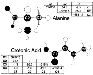
2-1 Molecular structure and Hamiltonian parameters for alanine

and crotonic acid. The chemical shift of each carbon nucleus is given

in the corresponding diagonal element while the coupling strengths are given by the off-diagonal values. All values are in Hertz, and they were

measured in a 300 MHz (-7 T) magnet. ... 24

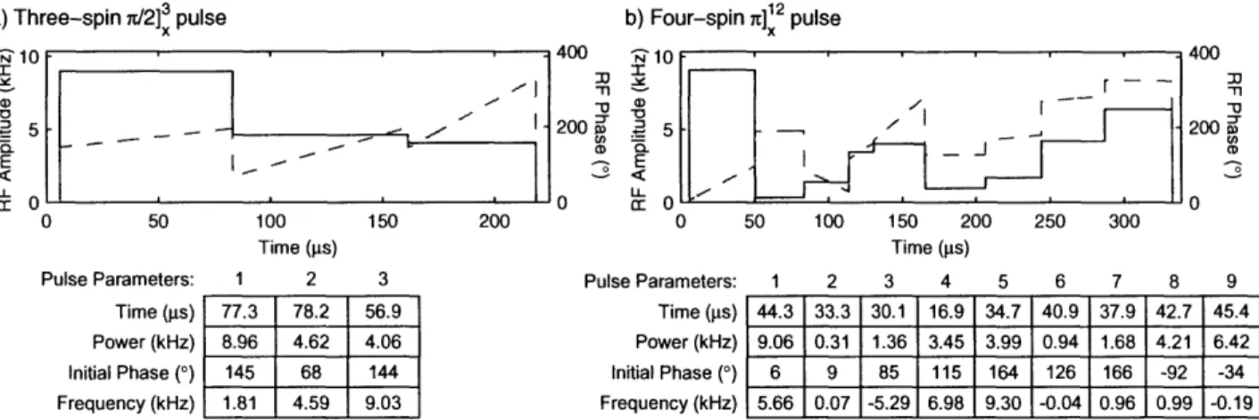
2-2 Ideal RF waveform for two example pulses. The solid (dashed) line is the amplitude (phase) of the waveform. Changes in the transmit-ter frequency (within a single period) were implemented by a discrete linear phase ramp. The sharp discontinuities occur at the transitions between periods. Substantial filtering of these high frequency compo-nents (smoothing of the shape) has little effect on the gate fidelity. In order to experimentally implement the pulse, it is converted into a discrete series of amplitudes and phases (order 1K long) by sampling the ideal waveform at a constant rate. Details of the pulse parameters (as per Eqn. 2.24) are listed below each waveform. Due to experi-mental implementation issues, a 6 ,us period with zero RF power (i.e., Hext = 0) is needed before and after the pulse and must be included

to produce the desired propagator. ... 28

2-3 Exploration of achievable fidelities. The plot shows the

maxi-mum fidelities found for a 7r/2]2 alanine pulse as allowed RF power

and magnetic field strength were varied. The three lines correspond to the magnetic field strengths explored, as denoted by the legend. The dotted vertical lines mark the point of the minimum chemical shift difference at each of the three field strengths. Using ideal experimen-tal control in a 800 MHz magnet, a single-spin gate fidelity reaching

0.99999 is potentially realizable. ... 29

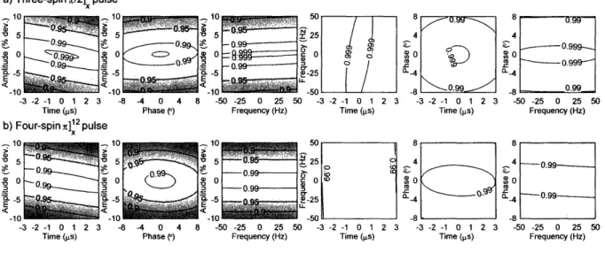
2-4 Gate fidelity vs. variations in experimental parameters. The experimental parameters were varied over the range of expected errors, demonstrating that both the alanine and crotonic acid pulses are most

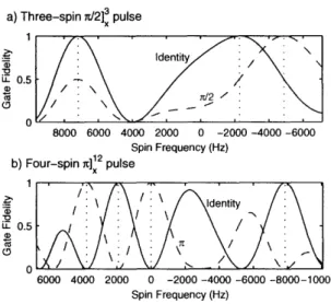
2-5 Gate fidelity vs. spin frequency. The gate fidelities of two example pulses were calculated as a function of the resonance frequency of a test spin. The frequency was varied in the range of chemical shifts of the molecules. The solid (dashed) line is calculated with identity (desired transformation) as the theoretical transformation. The vertical dotted lines denote the actual chemical shifts for each spin. As can be seen, the gate only works when the test spin is at the appropriate resonance

frequency ... 31

2-6 Feedback loop for correcting experimental RF waveforms. Dis-torted signals arriving at the carbon coil are detected and digitized through the proton coil. The difference between the measured RF wave and the desired wave is then calculated, resulting in a fixed wave that is then retransmitted to the coil. The loop continues until the

shape of the fixed wave produces the desired signal at the carbon coil. 33

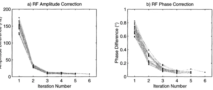
2-7 Improvement of errors in digitized RF waveforms. The errors from a test sample of 25 waveforms are plotted here as a function of the feedback loop iteration number. The errors are the mean absolute differences between fits to the digitized waveform and the ideal wave-form. Three to four iterations were typically sufficient to improve the

RF shape ... 34

2-8 Distorted and corrected RF amplitudes. The solid line repre-sents the desired shape, while the dashed and dotted-dashed lines cor-respond to the initial measured waveform and the final one (after two iterations of the feedback code) respectively. The high frequency tran-sients present at the transitions between periods have little effect on

the overall performance of the gates. ... 35

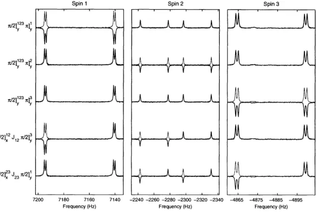
2-9 Spectra resulting from different sequences of pulses applied

to the thermal equilibrium density matrix

=

All sequences are read from left to right. The reference spectra

(re-sulting from a pulse applied to all 3 carbons) is also shown (grey)

for reference. Although the chemical shift is of order 1, no significant phase evolution is seen. Selective coupling sequences are also demon-strated. The phase correction used for all the spectra is strictly the same for all of them and is done such that the reference spectrum (/2

pulse on all the spins at thermal equilibrium) is perfectly absorptive. 36

3-1 Radio-frequency inhomogeneity profile. The RF inhomogeneity in the carbon channel was measured using a spin nutation experiment. The resulting decaying signal was Fourier transformed to distill the various RF nutation frequencies present in the sample. The dotted line is the plot of the Fourier transformation, and it is the measured RF inhomogeneity profile. The solid gray line is the profile that was used to design pulses compensated for RF inhomogeneity, and it was

3-2 Simulations of compensated and uncompensated pulses as a function of radio-frequency strengths and distribution widths. The dashed lines correspond to compensated pulses, while the solid gray lines denote uncompensated pulses. The left plot shows how the compensated pulses maintain high fidelities even when the RF strength is scaled from the ideal value. The plot on the right simulates the same pulses as a funcion of the scaled width of the RF inhomogeneity profile. These results demonstrate the improved fidelity of the compensated pulses for all but the narrowest RF distributions. At the small widths, the RF profile would no longer be inhomogeneous, eliminating the need

for the compensated gates ... ... 45

3-3 Eigenvalue spectrum of the simulated superoperator for a test gate and the radio-frequency inhomogeneity profile shown in

Fig. 3-1. The dots are the exact eigenvalues of S while the crosses are

the ones obtained by using the first order perturbation analysis. The zoom box shows some of the detail in the left-hand side of the plot. The additional trend line drawn in the zoomed plot emphasizes the

fact that the larger the phase shift, the larger the attenuation ... 48

3-4 Eigenvalue spectrum of the simulated superoperators corre-sponding to a compensated and uncompensated pulse. The dots correspond to the uncompensated gate, while the crosses corre-spond to the compensated one. Note that the crosses basically lie on the unit circle while the dots are spread inside, confirming the

closer-to-unitary behavior of the compensated gates. ... 49

3-5 Eigenvalue spectrum of the simulated superoperator for the

symmetric radio-frequency inhomogeneity profile. The dots are

the unperturbed eigenvalues and the crosses are the ones computed by using first order perturbation theory. The symmetry in the distribution mainly results in some attenuation of the eigenvalues with no phase shift. The zoom box allows more detail to be seen for the eigenvalues

close to -1. ... 51

4-1 Logical network for the entanglement transfer experiment. The four spins are represented by the four horizontal control lines, where each line is labelled on the left by the input state superscripted by the spin's index (where "1" indicates that the spin is depolarized

and E+ indicates that it was part of the pseudo-pure state). The

pseudo-pure ground state on spins 2 and 3, p -23 100)(00[, is converted

by an entanglement operation on the same spins to obtain p23 t

2(00) + Ill))((00I + (11). This state is then transfered to spins 1 and

4 by using swap gates. ... 56

4-3 Experimental density matrices. From left to right are shown the

real part of the reconstructed density matrices of the initial pseudo-pure p , spins 2&3 entangled pEnt and spins 1&4 entangled pEt (in normalized units). The bottom row of density matrices is obtained from the top row after having traced over the two ancilla spins. The rows and columns represent the standard computational basis in binary order, with (00001 starting on the leftmost column and (11111 being

the rightmost column. ... 59

4-4 Logical network for the entanglement swapping experiment. The four qubits are initialized to the full pseudo-pure state 1+?)12 ()3 4

where

4+)

map the Bell basis to the computational one. That operation followed by a strong measurement in the computational basis mimicks a strong

measurement in the Bell basis ... 61

4-5 Real part of the initial density matrix (product of singlet

states). The rows and columns represent the standard computational

basis in binary order, with (00001 starting from the leftmost column

and (11111 being the rightmost column . . . .... 62

4-6 Bell states. For the sake of convenience, the labels of the spins have been switched so that the pattern characteristic of the Bell states is more clear. Now the ket 10000) should be interpreted as 10)2 0 10)3 0 0)1 0 10)4. One can see that the measurement results in an equal mixture of the four Bell states. For clarity, we zoomed on the sub-matrices along the diagonal to show the Bell states more clearly

(') =

(100) ± 111)),

q

_{:) = (}

_{1) 110>))) ...}

_.

₆₃

4-7 Entanglement transfer efficiency versus the strength of the

measurement. For a = 1 the correlation between the simulated Pout

and the theoretical density matrix is equal to 0.93. This value being less than 1 is due to the non perfect experimental input state and to

the coherent errors contained in UBellMap ... . 64

5-1 Molecule of 2,3 dibromothiophene with the two protons

la-beled 1 and 2. The chemical bonds among the atoms are indicated

by double parallel lines, and a transparent "dot-surface" used to

indi-cate their van der Waals radii ... 71

5-2 Redfield kite structure of the relaxation superoperator

ex-pressed in the transition basis (TABLE I). The shaded area

cor-responds to blocks of different coherence order which are effectively

5-3 Three different estimates of the relaxation superoperator of 2, 3 dibromothiophene in the transition basis, indexed as

in-dicated in Table I. (a) Relaxation superoperator obtained from a

least-squares fit, without the complete positivity constraint, of the ex-ponential exp(-z(1t+ R) tin) to the propagators Pmat the correspond-ing times (tl = 0.4, t2 = 0.8, t3 = 1.6, t4 = 3.2 s) with respect to the

symmetric Redfield kite relaxation superoperator matrix RZ, starting from the results of Richardson extrapolation (see text). (b) The re-laxation superoperator obtained from a fit to the same data and with the same starting value of R, but with the complete positivity con-straint included in the fit. (c) The relaxation superoperator obtained by assuming that 7-( and R7 commute, and using the average of the estimates obtained by taking the logarithms of the absolute values of the eigenvalues of the propagators over all four time points as the final

estimate (see text) ... 74

6-1 Quantum network for the DFS-QEC concatenation scheme. The second physical qubit from the top is the data qubit, while the first physical qubit and the third grouped with the fourth one are the ancillae and the logical ancillae respectively. HL denotes a logical Hadamard operation [1. The engineered noise implemented incoherent independent z noise on qubits 1, 2 and 3, in addition to a strong

collective z noise on qubits 3 and 4 only. ... 83

6-2 Pulse sequence for the DFS-QEC scheme. The blocks represent selective one-qubit rotations while the bell-shapes represent magnetic field gradients. Each pulse is a strongly modulating pulse designed to be robust against RF inhomogeneity, and corrected using a feed-back loop to counteract systematic errors. The experiment contains 83

pulses, 13 gradient pulses and lasts roughly 130 ms ... 84

6-3 Pulses and magnetic field gradients sequence to implement

the noise. The black boxes represent r pulses. The internal

Hamil-tonian is thereby refocused while encoding k-space components along different directions for the different qubits. The collective noise was also implemented using a magnetic field gradient in the z direction to-gether with the weak z noise on the third physical qubit, thereby

im-plementing the noise model b. Here T = 35 us, G3 = 60 x 2.6% G/cm,

G4 = 60 x 20% G/cm, and G1 and G2 were calibrated to yield the same

attenuations as for G3given the geometry of the sample (Lz 1.6 cm,

Lx = Ly z 0.5 cm) and unequal gradient strengths (Gma _{x = 60 G/cm,}

6-4 Experimental results. The dots correspond to the 3-qubit QEC scenario with independent z noise only while the asterisks correspond to the same scenario but with additional strong collective noise, and k(t) = ko(t). The squares correspond to the No QEC scenario and the diamonds to the DFS-QEC scheme. There is an error bar of ± 0.02 for each data point which is not diplayed here for the sake of clarity. (a) Entanglement fidelity results (see text for an explanation of the different effects). (b) Average normalized polarization of the output

states (see text). ... 87

6-5 Simulation of the DFS-QEC concatenation experiment. Most of the experimental features, i.e. the "hump" in addition to the drop of the QEC-DFS scenario compared to the QEC alone are reproduced. The "hump" is due to an imperfect initialization of the ancillae (see text for a detailed explanation). The drop mentioned above on the other hand is primarily due to coherent and incoherent errors because of the longer sequence (more pulses) for the QEC-DFS scheme. We

add here for clarity that k(t) = ko(t) ... 89

6-6 Illustration of the "hump" effect (ideal simulation). The max-imum correlation for the QEC case is - 1.00341 as predicted by the

List of Tables

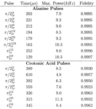
2.1 Summary of relevant characteristics for an example set of

transformations. The three columns list the pulse duration (in s), maximum power (in kHz), and the gate fidelity of the simulated pulse. While the maximum power is relatively large, all powers are experimen-tally feasible. The pulses designed for the crotonic acid sample require longer times and yield lower fidelities due to the decreased chemical

shift separation and increase of coupling strengths. ... 27

2.2 Summary of experimental data for the Alanine sample. For each of six 7r/2 pulses, the experimentally determined density matrix is compared with the expected result. The first column (No Pulse) confirms that the experimental and expected inputs have almost unit overlap. Each of the other headings denote which spins are rotated by 7r/2. In each case, the projection and attenuated correlation for each pulse is averaged over the three inputs Il + I + I3, for j = x, y, z. Because all pulses are short in comparison to the natural decoherence times, the attenuation gives an indication of the relative significance of the coherent and incoherent errors. Uncertainties arising from errors

in the tomographic density matrix reconstruction are of order 1%. 37

3.1 Summary of experimental results. The metrics C, A, and CA,

refer to the correlation (or projection), attenuation, and attenuated correlation (CA = C. A). The superscripts specify whether the pulses employed were compensated or uncompensated for RF inhomogeneity, while the angle brackets denote that the reported quantities are means over the three input states tested for each transformation. In the case of the spin-rotation values, the quantity reported is the average of all

the spin-rotation results. ... 52

3.2 Experimental results of spin-rotation gates. The metrics C, A, and CA, refer to the correlation (or projection), attenuation, and

atten-uated correlation (CA = C .A). The superscripts specify whether the

pulses employed were compensated or uncompensated for RF inhomo-geneity, while the angle brackets denote that the reported quantities are means over the three input states tested for each transformation. The spin-rotation pulses tested were 7r/2 and 7r rotations of the carbon

5.1 Table of operators (versus Cartesian basis) of the transition

basis used for the density and superoperator matrices, the

corresponding matrix indices and their coherence orders (see

Chapter 1

Introduction

Computers today play a fundamental role in science and industry. During the last few decades, a tremendous increase in the performance of computers has been ob-served. As a matter of fact, the power of computers has increased exponentially with the number of years, as predicted by Moore's law. The massive increase of com-putational power represented by contemporary computers is a direct result of the

successful drive to build electronic devices on a smaller and smaller scale. When the size of the components approaches atomic dimensions, quantum mechanics becomes an unavoidable factor. This theory has revealed itself to be one of the most

suc-cessful in the history of science, in spite of many features that defy common sense.

Nevertheless, even with so powerful a theory, great obstacles to improve conventional

computers will soon arise due to the unavoidable bounds of miniaturization. For

this reason, rmembers of the scientific community started to work on improving the capabilities of- a computer from a totally different angle.

In the early 1980s, scientists, including Richard Feynman [2], thought about pos-sible schemes to exploit the laws of quantum physics to their rational ends. This led to the idea of a "quantum computer", i.e. a computer whose functional principles would be based on the quantum mechanical laws. Though a functional quantum computer still lies beyond the grasp of current technology, a succession of theoretical and practical advances suggests some heartening progress towards that goal.

In a quantum computer, information is not stored as a string of ones and zeros, but in a quantum mechanical wavefunction, containing information for instance about spin directions or photon polarizations, that can represent superpositions of states. Within this context, the term "bit" is now replaced by "qubit", and the latter quantity can be in the 0 and the 1 state at the same time. Because the quantum dynamics of a system are linear, if a n-qubit system is prepared in a superposition of 2' states a

quantum computer acting on it will perform 2n _{operations, or computations, at once.}

Research in the field of quantum computing really exploded when Shor published a paper describing an algorithm that would enable the factorization of an integer into primes exponentially faster than the best classical algorithm known so far would [3]. This factorization problem lies in the heart of the RSA cryptographic system, which is used very heavily. This discovery had an enormous impact, given that the security of encryption systems that depend on the difficulty of performing this operation could

someday be compromised. Building a quantum computer however remains a very technically challenging problem, requiring both precise control of a quantum system and isolation from the noisy effects of the environment. These two requirements are some of the main obstacles in the quest for a working quantum computer.

In this context, this thesis addresses some aspects of the different problems encoun-tered in the control of a quantum information processor, namely the coherent control of the quantum system dealing with unitary dynamics only, and then in the presence of incoherent and decoherent noise. We report here a new and original technique based on time-dependent control fields tailored to perform accurate and selective unitary operations on small nuclear spin systems (up to 10). The method is then extended to counteract the main source of incoherence in liquid state nuclear magnetic resonance (NMR) experiments, namely radio-frequency power inhomogeneity (chapter 3). The sequences obtained are modular, i.e. their performance compared to a desired trans-formation does not really depend on the input state, and their calculated fidelities represent today the state of the art control of homonuclear spins. Simple experiments are reported in order to confirm their performance. Two more sophisticated experi-ments, namely an entanglement transfer and an entanglement swapping experiment, using 4 qubits are then carried out as benchmarks to illustrate the performance of the technique and its extension (chapter 4). This leads us finally to the final and very important problem of decoherence. Methods based on quantum process tomogra-phy (QPT) are developed to acquire further qualitative and quantitative information about the underlying sources of incoherence and decoherence (chapter 5). The latter techniques are furthermore illustrated and tested through the measurement of the noise generators of a two-qubit system. As confirmed by this measurement, one can in general expect in a quantum computer some partial symmetry in the noise pro-cess. In chapter 6, we investigate the concatenation of a decoherence-free subspace (DFS) scheme, which counteracts completely the collective part of the noise, with a quantum error correction code which corrects for the remaining part to first order. We thereby report the first experimental concatenation of different quantum infor-mation protection schemes. As a whole, this work represents one of the first steps in the development of precise control of quantum information both in the presence of incoherence and decoherence.

Chapter 2

Quantum Control

The past decade has seen a substantial interest in improving coherent quantum con-trol. Coherent control has origins in both nuclear magnetic resonance (NMR) [4, 5] and optical spectroscopy [6, 7]. For an overview of advances in both fields, the reader is referred to [8]. Since coherent control's inception, many different techniques have been used both to improve selectivity and to reduce the duration of control pulses. For spin systems, the Fourier transform has been used to approximate the excitation profile in the limit of low power and no spin-spin couplings [9] and more complete analytic solutions have been developed to aid in general pulse design and analysis

[10, 11, 12, 13, 14, 15]. Alternatively, very sophisticated shaped pulses have been

designed using a variety of computer-aided methods [16, 17] or feedback from system observables [18]. Equivalent analytic theories [19, 20], computer-aided methods [21] and feedback techniques [22, 23] have also been developed by the optics commu-nity. Similar techniques are also used in other fields such as the control of trapped

ions [24, 25].

The development of liquid-state NMR systems as prototype quantum informa-tion processors [26, 27] has enabled experimental demonstrainforma-tion of quantum algo-rithms [28, 29, 30], quantum error correction [31, 32], and quantum simulations [33]. These experiments built upon well-established spectroscopic techniques developed over the past four decades, such as using low-power (soft) shaped radio-frequency (RF) pulses to obtain selective operations. However, the selective pulses employed to date have the disadvantage that low power implies long duration. This not only in-troduces errors due to relaxation, or decoherence, but also allows significant evolution under the action of the internal Hamiltonian. In the past, this evolution was rarely of concern because there was little importance placed on implementing a particular operation. For example, in spectroscopy there are entire classes of propagators that selectively excite a single spin from its equilibrium state, but for applications such as quantum computing the transformation must act as expected for all input states.

1_{Parts of this chapter were extracted from E. M. Fortunato, M. A. Pravia, N. Boulant, G.}

Teklemariam, T. F. Havel, and D. G. Cory, "Design of strongly modulating pulses to implement precise effective Hamiltonians in quantum information processing," Journal of Chemical Physics,

A second problem with soft-pulse techniques is that selective pulses simultaneously applied to different spins interfere with each other, thus causing significant deviation from the desired action [34]. To address some of these problems, several groups pre-calculate these errors and incorporate corrections into their analysis and pulse design

[35, 36]. However, not all errors can be corrected using these techniques2, and it

would be preferable to average out unwanted evolution by the use of strong control fields, so that no additional corrections are required.

In this chapter, we present a procedure for finding high-power pulses that strongly modulate the system's dynamics to produce precisely a desired spin-selective unitary propagator. These operations, or gates, allow arbitrary rotations of each spin around independent single-spin axes, while refocusing the internal evolution. They are "self-contained", in the sense that they can be placed back to back in longer sequences

without requiring additional computational resources or post-experiment corrections3.

By using high-power, pulse durations are decreased by almost an order of magnitude, thereby significantly reducing the effects of relaxation. The simulated gate fidelities

of the pulses are high, reaching past 0.9999 on the three-spin system 1 3C-alanine

placed in a 800 MHz magnet. Finally, the use of strong modulation also allows the incorporation of robustness against slowly varying or time-independent incoherent errors such as those caused by RF inhomogeneities [37, 38, 39]. Our control methods are the first to combine all of these features.

The pulses presented here have been applied in recent Quantum Information Pro-cessing (QIP) experiments to demonstrate algorithms [30], study notions of measure-ment [40], and test new methods for noise control [41]. They promise to be increas-ingly useful in future NMR QIP experiments, where larger numbers of qubits will necessitate increasing the number of homonuclear spins. In addition, these methods can be adapted to develop improved pulses for selective spectroscopy [42] and imag-ing [43]. Finally, although presented within the context of NMR, these methods are applicable to any system where the total Hamiltonian is well known and the external degrees of freedom allow for universal control, both requirements of any quantum information processor.

2.1 Metrics of Control

In designing gates for controlling quantum information, a metric is required to judge how well a specific implementation compares to the ideal, desired transformation. A metric of a gate's performance should describe the quality of a general transformation, including the possibility of non-unitary evolution. Unfortunately, such information is not directly accessible by experiment, so we choose a metric comprised only of sets of state measurements. For an input state, Pin, the ideal transformation maps the

2

For instance, not all errors can be represented as a composition of phase shifts, az z couplings and ideal 7r/2 or 7r pulses.

3

system to a theoretical output state, Pth, i.e.,

Pin U Pth Pth-(2.1)

On the other hand, a simulated or experimentally implemented control sequence will produce a different output state, Pout, i.e.,

Pin Pout. (2.2)

Noting that p is Hermitian, the projection between these two states, defined as trace(pth pout)

P(Pth, Pout) trace(pth Pout) (2.3)

vtrace(pth)trae

(Pout

)

quantifies how similar in 'direction' the two states are. This metric is analogous to the dot product between two vectors, varying from -1 for anti-parallel states to 1 for identical states. A value of zero indicates orthogonal density matrices. In order to account for non-unitary evolution, a second term multiplies the projection yielding the attenuated correlation, namely,

t'race(p"t

C(Pth, Pout) = P(Pth, Pout) trace (24)

trace(pth Pout)

=race (pth)trace (P~ (2.5)

The projection and the attenuated correlation serve as metrics for state fidelity. The gate fidelity, F, of a transformation is defined as

F = C(pth, Pout),

(2.6)

where C represents the average attenuated correlation over an orthonormal set of input density operators (i.e., Trace[pjpk] = jk) that span the Hilbert space. It

should be noted that F is maximized (with a value of one) when the implemented and ideal transformations are the same, and is insensitive to differences in the global phase between the ideal and implemented transformation.

We can derive a useful alternate form for the gate fidelity in terms of the ac-tual and theoretical transformations instead of the input-output state relations. This form is both easier to compute and has intuitive appeal in that knowledge of the transformation can be directly translated to gate fidelities. First we assume that our ideal transformation is unitary, and the implemented transformation is a completely positive, trace-preserving linear map [44]. In other words, the implemented transfor-mation takes density operators to valid density operators. Under these assumptions, Eqns. 2.1 and 2.2 are explicitly given by

and

Pout ApinA, (2.8)

where the A, satisfy the trace-preserving condition

S£

We now show that the gate fidelity reduces to

F =

5

where N is the dimension of the Hilbert space. Using the normalized Pauli basis, aj, as the orthonormal input density operators and the cyclic properties of the trace, Eqn. (2.6) becomes N2 F = E Tr[(UthjUth)( A,crjAt)]/N2 (2.11)

j=1

/

Expanding the product of UthA, in terms of the orthonormal Pauli basis (UthA, =

Ek By k), yields

=

S

B

j,

k m

- B B*Tr[jUkUajm]/N 2.

(2.14)

jpkm

Because the a Pauli basis is orthogonal, only terms where k = m contribute. There-fore, Eqn. (2.14) reduces to

F =

5

If Oak is not proportional to identity, it will anti-commute with exactly half the aj terms

in the sum, while commuting with the other half. Therefore, two sets of terms cancel and have no contribution to F. Defining al to be the element that is proportional to identity, Eqn. (2.15) further reduces to

F = IB 12_Tr[uj

_j]/N

=

S

IBI

/N

I

/N.

This is clearly equal to Eqn. 2.10. Thus, the gate fidelity corresponds to how well the actual transformation reverses the action of Uth. In this form it is obvious that the gate Fidelity is independent of which orthonormal basis of input states is used as pi, as long as it has the same properties as the Pauli basis.

2.2 Designing Gates for Controlling Quantum

In-formation

In the standard model of quantum computing, an algorithm can be expressed as a series of unitary operations that maps a set of input states to a particular set of output states. The physical implementation of an algorithm requires the use of a quantum system with an Hamiltonian that contains a sufficient set of externally controlled parameters to allow for the generation of a universal set of gates [45]. The task of control is to find a time-dependent sequence of values for these control parameters that modulates the system's dynamics in order to generate a particular gate to the required precision.

Given a control sequence, solving for the effective Hamiltonian is straightforward. Unfortunately, going the other way is much more difficult. That is, finding a RF waveform that produces a propagator with desired properties is an inverse problem. Traditionally, analytic techniques, such as average Hamiltonian theory [5], have been used to deterrmine an appropriate control sequence. With modern computer resources, numerical methods provide a more efficient and accurate solution to this problem.

2.2.1 NMR Spin System

As an example, liquid-state NMR is used to demonstrate how to find control sequences to implement particular gates. In NMR, spins in a large static magnetic field (in our case, -7 T) are controlled via external RF pulses. The internal spin Hamiltonian is composed of both Zeeman interactions with the applied field modified by electron screening (chemical shift) and scalar couplings with other spins. Together these pro-vide the QIP requirements of addressability and conditional logic respectively. In terms of spin operators, the internal Hamiltonian is

n n n

Hit

= WkI

+

2

E

JkIk.Ij,

(2.18)

k=l j>k k=1

where wk represent the chemical shifts of the spins, Jkj the coupling constant between spins k and j? and n is the number of spins. The test molecules used throughout this document are shown in Fig. 2-1, along with the relevant internal Hamiltonian values. The external Hamiltonian describing the coupling between the spins and an

oscil-L C1 I C2 I C3 I ] M7.8 54.1 -1.3 C1 -2286.5 35.0 C2 -4881.4 C3 Alanine Crotonic Acid C1 3767.5 I C2 72.4 0 C3i -1.3 69.7 915 .'8-C4 7.0 -1.6 41.5 -7850.4 .C1I C2 C3 C4 ... .. ... ... ... .. ... ...

Figure 2-1: Molecular structure and Hamiltonian parameters for alanine

and crotonic acid. The chemical shift of each carbon nucleus is given in the

corre-sponding diagonal element while the coupling strengths are given by the off-diagonal values. All values are in Hertz, and they were measured in a 300 MHz (7 T) magnet.

lating RF field generated by a single transmitter is

n

Hext(WRF, O, W, t) = -E ei(wRFt+IZ k i e( R F t+ ~) I k (2.19) k=l

where WRF is the transmitter's angular frequency, X the initial phase, and w the

power4. Of course, additional species can be added by including appropriate terms

in Hint and an additional Hext for each additional RF field.

2.2.2 Numerical Search Method

Using this knowledge of the internal Hamiltonian and the form of the external Hamil-tonian, the parameter values that generate the desired gate must be determined. Here,

a quality factor Q = 1 - F is minimized by searching through the mathematical

parameter space using the Nelder-Mead Simplex algorithm [46]. While this function has many local minima, the Simplex algorithm often succeeds in finding satisfactory solutions. Our goal is to show that sufficient, implementable control sequences can be found. Finding the optimal solution is much more challenging and based on our system and control parameter values, is not expected to improve pulse performance significantly. We have parameterized the control sequence as a cascade of RF pulses with fixed power, transmitter frequency, initial phase, and pulse duration (). As will be seen, this is a particularly convenient and completely general parameterization,

4_{Actually, w equals a spin's nutation rate caused by a RF field. Because this parameter is}

experimentally controlled by attenuating the RF power, it is commonly referred to as the pulse power.

but we make no claims that it is the only, nor necessarily the best choice. If the RF power is constant over the duration of a pulse, i.e., the pulse's amplitude is square,

the total Hamiltonian Htot = Hint + Het can be made time-independent by

transform-ing into the frame that rotates at the frequency of the transmitter. This allows the Liouville-von Neumann equation of motion to be solved by a single diagonalization. Initially, the starting density matrix is the same in both frames (p(0) = p(O)), so that at the end of the pulse, the density matrix in the new frame is given by

P(T) = e-iHeffTp(0)eiHef f, (2.20)

where Heff is the effective Hamiltonian in the new frame [47]. Transforming this density matrix back to the original frame gives

p(T) = Uz(T)-le-iHffTp(O)eiHeffrUz(T), (2.21)

where

Uz(T) = (eiwRF k= IkT). (2.22)

Therefore the transformation in the original rotating frame is given by

Uperiod(T) =

Ul( )e

_iHeffT.

_(2.23)

Because the evolution under the whole sequence is given in the original rotating frame, no additional resources are required to concatenate pulses, nor is any mathematical correction required at the end of an experiment.

Cascading these periods yields the net transformation

N

Unet = I| U (Tm)e iHeff( gtwRF m )Tm (2.24)

m=l

where the index m refers to the mth period, i.e., to the mth square pulse, with a

corresponding set of 4 parameters. In other words, N constant amplitude pulse

periods, each with a different transmitter frequency and initial phase, are applied in series. Clearly, a single period is not sufficient to generate an arbitrary transformation; therefore the number of periods is increased until a suitable net transformation is found. Using desktop computing resources, this yields convergence times for three-and four-spin systems that are typically seconds to minutes.

In addition to the desired propagator, Uideal, an initial set of starting parameters

for the pulse shape is required. While this initial guess must be reasonable (i.e., in the vicinity of the solution), many different starting points typically converge to equally deep minima. We have observed that the number of acceptable solutions for this parameterization is very large, allowing experimental implementation issues to be considered. For example, experimental limitations do not allow arbitrarily high powers or frequencies to be implemented. To keep the algorithm from returning infeasible solutions, a penalty function that increases as the parameter value moves towards infeasible solutions is added to the quality factor. Penalty functions are also

used to guide the algorithm towards more favorable pulse solutions. In our case, penalties are placed on high powers, large frequencies, and negative- or long-time periods.

2.2.3 Gate Simulations

The methods described above were used to obtain a set of pulses that implement each of a set of important single-spin gates. To study the performance of these gates, propagators for each of the pulses were simulated under different conditions. In the first set of simulations, the pulse performance was calculated for ideal implementa-tions using current experimental condiimplementa-tions. Second, the gate fidelity was simulated as a function of systematic distortions of the pulse parameters. From these results, the relative importance of implementation precision is determined. A final set of cal-culations showed how a pulse can generate quite different evolutions as the resonance frequency of a test spin is varied over a range of chemical shifts.

Ideal Pulse Simulations

Pulses were created for three- (3C-labeled alanine) and four- (1 3C-labeled crotonic

acid) spin homonuclear systems. The chemical shifts and scalar coupling constants for each of these systems are listed in Fig. 2-1. As a representative set, each of the single spin 7r/2, and nearest-neighbor paired 7r pulses were simulated with the relevant characteristics summarized in Table 2.1 and example waveforms shown in Fig. 2-2. The duration of the pulses is on the order of 200 ,us for the three-spin system and 420 Us for the four-spin system, both significantly shorter than those that could be obtained using low-power pulses. The average fidelities for each system are 0.9995 and 0.995, demonstrating that, at least under ideal conditions, control sequences that implement the desired transformation with high fidelity can be found.

The ultimate goal of control in quantum computing is to attain fault-tolerant com-putation. While it has been proven that perfect control is not required [48], estimates of the precision needed vary from 0.9999 to 0.999999 depending on the assumptions used. These simulations predict an achievable level of control that approaches the most optimistic estimates for fault- tolerant computation. As expected, the pulse duration decreases with increasing chemical shifts dispersion (selectivity condition) and, for the case that Jjk << Iwk - Wjl, the fidelity of the sequence decreases with

increasing ratio of the couplings (bilinear terms) to chemical shift. Exploring Achievable Fidelities

One of the most important results in QIP is the discovery that indefinite, fault-tolerant computation is possible when the gates used to correct for experimental errors have a fidelity above a certain level [48]. The simulated single-spin gate fidelities of the alanine pulses in Table 2.1 reach the lower end of the threshold, but it is important to explore further what fidelities are achievable (with the present method) in situations with extended experimental capabilities. For this purpose, we extensively explored

Pulse Time(Ms) Max. Power(kHz) Fidelity Alanine Pulses 7r/2]x /2]2 7/212 7T/2]23 7]12 7] 23 X]~ 7r/2]1 7r/2]2 7/2]3 /2]4 fr] 12 7r] 23 7r] 34 X]~ 202 7.9 221 9.3 212 9.0 194 8.5 179 9.2 163 10.3 252 8.0 129 10.3

Crotonic Acid Pulses

389 8.5 610 4.8 392 6.3 559 7.6 326 9.0 315 11.3 345 8.4 0.9995 0.9995 0.9995 0.9995 0.9995 0.9995 0.9996 0.9997 0.9930 0.9957 0.9950 0.9923 0.9963 0.9932 0.9962

Table 2.1: Summary of relevant characteristics for an example set of

trans-formations. The three columns list the pulse duration (in ts), maximum power (in kHz), and the gate fidelity of the simulated pulse. While the maximum power is relatively large, all powers are experimentally feasible. The pulses designed for the crotonic acid sample require longer times and yield lower fidelities due to the decreased chemical shift separation and increase of coupling strengths.

a) Three-spin r/2]3 pulse b) Four-spin ]12 pulse ro 10 400 i 400 E I ' I ---LL . , , -Ic ' ' 0 ' 200 0 c 51500 150 200 0 50 100 150 200 250 300 Time (s) Time (s)

Pulse Parameters: 1 2 3 Pulse Parameters: 1 2 3 4 5 6 7 8 9

Time (S) 77.3 78.2 56.9 Time (s) 44.3 33.3 30.1 16.9 34.7 40.9 37.9 42.7 45.4

Power (kHz) 8.96 4.62 4.06 Power (kHz) 9.06 0.31 1.36 3.45 3.99 0.94 1.68 4.21 6.42

Initial Phase () 145 68 144 Initial Phase () 6 9 85 115 164 126 166 -92 -34

Frequency (kHz) 1.81 4.59 9.03 Frequency (kHz) 5.66 0.07 -5.29 6.98 9.30 -0.04 0.96 0.99 -0.19

Figure 2-2: Ideal RF waveform for two example pulses. The solid (dashed) line is the amplitude (phase) of the waveform. Changes in the transmitter frequency (within a single period) were implemented by a discrete linear phase ramp. The sharp discontinuities occur at the transitions between periods. Substantial filtering of these high frequency components (smoothing of the shape) has little effect on the gate fidelity. In order to experimentally implement the pulse, it is converted into a discrete series of amplitudes and phases (order 1K long) by sampling the ideal waveform at a constant rate. Details of the pulse parameters (as per Eqn. 2.24) are listed below each waveform. Due to experimental implementation issues, a 6 Us

period with zero RF power (i.e.,

Het

must be included to produce the desired propagator.

the parameter space of a r/2]2 alanine pulse by running hundreds of Simplex searches, each time varying the initial guess, the penalty function for the maximum allowable RF, or the magnetic field strength. Fig. 2-3 summarizes the findings. The three curves represent the results for each of three magnetic field strengths tested. The stronger fields allow pulse solutions with higher fidelities because of the increased chemical shift dispersion. The stronger fields cause the spin frequencies to widen, allowing more spectral room for addressability and control. Fidelities also tended to increase with the maximum RF power for values between -l Hz and -104 Hz. At low powers, the RF control is insufficient to average out the internal Hamiltonian, resulting in low fidelities. At high RF control power, the strength of the RF dominates the internal

Hamiltonian, resulting in the desired control. The three vertical dotted lines (one for each field) indicate where the smallest chemical shift frequency differences fall relative to the RF power strength. As expected, the sharp increase in the fidelities occurs when the RF power is able to dominate the chemical shift terms in the internal Hamiltonian. The maximum gate fidelity in the plot is close to 0.99999, suggesting that, for the single-spin gate examined, the fault-tolerant limit is potentially achievable.

It is important to emphasize that the maximum achievable fidelities of Fig. 2-3 represent the best gates achieved using the current pulse parameterization and available search method and resources. The results do not preclude other methods

Maximum Fidelity Found for a Three Spin 0.999 0.99 _0 LL 0.9 0. 10° 10' 102 10 104

Maximum Pulse Power (Hz)

Figure 2-3: Exploration of achievable fidelities. The plot shows the maximum fidelities found for a r/2]2 alanine pulse as allowed RF power and magnetic field strength were varied. The three lines correspond to the magnetic field strengths explored, as denoted by the legend. The dotted vertical lines mark the point of the minimum chemical shift difference at each of the three field strengths. Using ideal experimental control in a 800 MHz magnet, a single-spin gate fidelity reaching 0.99999 is potentially realizable.

and pulse strategies from yielding higher fidelities.

2.3 Systematic Errors

The above results demonstrate how knowledge of the internal and the control Hamilto-nians can be used to design custom sequences for generating unitary transformations. The fidelities reported are around 0.999 for the typical systems of three and four qubits. It still remains however to estimate how sensitive these solutions are with respect to small errors in the control parameters. The simulations in this section report the robustness of the implemented gates versus some systematic variation or uncertainty of control parameters such as power, phase, time, frequency, chemical shifts etc... Although simulations of the pulses demonstrate that the gates are ro-bust against small deviations in some of the control parameters, a substantial loss of fidelity occurs when the RF amplitudes deviate in a systematic way from the pre-scribed values, the robustness decreasing with the number of spins. At the end of this section, we describe a feedback procedure that detects and corrects experimental deviations from the ideal RF shapes. The study and the development of tools aimed at counteracting incoherent errors is reported in the next chapter.

a) Three-spin c/23 pulse 8 4 -r -8 0 4 0-4 --3 -2 -1 0 1 2 3 -8 -4 0 4 8 -50 -25 0 25 50 -3 -2 -1 0 1 2 3 -3 -2 -1 0 1 2 3 -50 -25 0 25 50 Time (s) Phase (o) Frequency (Hz) Time (ps) Time (us) Frequency (Hz)

) Four-spin 4]12 pulse x 8 4 8 . O --4 -8 0 4 -4 -8 -3 -2 -1 0 1 2 3 -8 -4 0 4 8 -50 -25 0 25 50 -3 -2 -1 0 1 2 3 -3 -2 -1 0 1 2 3 -50 -25 0 25 50

Time (us) Phase (o) Frequency (Hz) Time (s) Time () Frequency (Hz)

Figure 2-4: Gate fidelity vs. variations in experimental parameters. The experimental parameters were varied over the range of expected errors, demonstrating that both the alanine and crotonic acid pulses are most sensitive to RF amplitude.

2.3.1 Variations in the External Hamiltonian

The external RF parameters are determined by a minimization procedure, suggesting that small variations of the external parameters should have little effect on the quality of the pulses. To check this assumption, the gate fidelity was calculated as each of the six pairs of the four control parameters were varied over a range of errors typical of an experimental implementation. As a sample set, one pulse for each of the two systems is presented here. The results shown in Fig. 2-4 demonstrate the natural robustness against typical variations in the initial phase, frequency, and duration of each period.

Clearly, the sequence is most sensitive to power variations. For the pulses listed in Table 2.1, if the power's amplitude is changed by 5% the average fidelity falls to 0.96 ± 0.01 for alanine pulses and 0.94 ± 0.04 for crotonic acid pulses. For the 25 pulses used in [41] the average fidelity at 5% amplitude deviation is 0.97 ± 0.02. For 10% deviation, the gate fidelity drops to 0.86 ± 0.03 for the alanine pulses and 0.81 + 0.12 for the crotonic acid pulses. This pulse sensitivity to RF amplitude suggests that RF inhomogeneity may be a leading cause of experimental errors. While techniques to select homogeneous regions are available [36, 49], the loss in signal to noise is significant, especially if multiple coils are used. Instead, because these errors are incoherent in nature, it is possible to design pulse sequences that refocus such

inhomogeneities (see chapter 3).

2.3.2 Variations in the Internal Hamiltonian

For NMR spectroscopy, the goal is to excite selectively spins in a band of frequencies leaving all other possible spins (with unknown precession frequencies) along the z

10 5 0 -5 -10 ED 'o a)_ a 2 E b n v _ _ n i v

a) Three-spin n/2]3pulse ID ' LL 0.5 n 8000 6000 4000 2000 0 -2000 -4000 -6000 Spin Frequency (Hz) b) Four-spin c]12 pulse 1*. * / Identity 00 6000 4000 2000 0 -2000 -4000 -6000 -8000-10000 Spin Frequency (Hz)

Figure 2-5: Gate fidelity vs. spin frequency. The gate fidelities of two example pulses were calculated as a function of the resonance frequency of a test spin. The frequency was varied in the range of chemical shifts of the molecules. The solid (dashed) line is calculated with identity (desired transformation) as the theoretical transformation. The vertical dotted lines denote the actual chemical shifts for each spin. As can be seen, the gate only works when the test spin is at the appropriate resonance frequency.

axis. This requires that the propagator for spins at any other frequency be, at most a phase change. With detailed knowledge of the internal Hamiltonian, the effect of the applied RF field needs only be considered at the resonance frequencies of the chemical species present in the given molecule. By relaxing the requirement that the average Hamiltonian be zero for all chemical shifts other than those in the band of excitation, a RF shape can be found that more efficiently implements the desired gate for the frequencies of concern yielding high-power yet selective pulses. To demonstrate this idea more clearly, the gate fidelities of the two sample pulses considered in this chapter

were calculated as a function of a test spin's resonance frequency. As can be seen in

Fig. 2-5, the fidelity is close to unity only near the resonance frequency for which the pulse was designed to work.

This stresses the necessity of having accurate knowledge of the system's Hamilto-nian. On the other hand, looking at the region immediately around the resonance we see the fidelity falls off quite slowly. This implies that small variations in the chemical shift do not significantly affect the fidelity of the pulses. For example, in the experi-ments presented below, the unwanted scalar couplings to the hydrogen atoms, which are equivalent to errors in the resonance frequency when these are left untouched, were automatically refocused by the control pulse. It should be noted that no con-straint was used to require this robustness, but that it results from the use of strongly modulating pulses. If this natural robustness is not sufficient, additional constraints can be added. However, it was found empirically that the robustness of the pulses versus chemical shift variations decreases as the number of spins increases (unless the

width of the window of resonance frequencies also increases). When considering a single nuclear species coupled with another species via the scalar coupling, this ob-servation suggests the use of dynamical decoupling [50] if the experiment is not too long (it leads otherwise to some nuclear Overhauser enhancement [47]) to average out these undesired couplings.

2.3.3

RF Waveform Feedback Correction

In the spectrometer originally used to test these new schemes, a digital waveform generator creates the desired shape. The signal is then amplified and routed to a

coil in the probe that is tuned to the carbon resonance frequency (75 MHz). The

sample is inserted in the coil, where it is exposed to the RF irradiation that generates the desired gates. Because of nonlinearities in the transmitter and probe circuits, the waveforms observed by the spins are distorted from the intended shapes. For a set of 25 sample waveforms, the mean absolute deviation between the observed RF amplitudes and the intended amplitudes was about 150 Hz, while the mean phase deviations were comparatively smaller, at about 0.7 degrees. Using Fig. 2-4 as a reference, one can expect that the phase errors cause negligible loss in fidelity. In contrast, the amplitude errors cause the RF nutation rate in each period to vary up to 4 percent for typical alanine pulses, resulting in a significant drop in fidelity. Simulations of alanine gates having errors of this magnitude have fidelities about 0.03 smaller than the fidelities of the ideal transformations, suggesting a need for improved RF shaping.

To correct the amplitude and phase errors, we used an iterative feedback pro-cedure to determine the prewarped RF waveforms that, when distorted through the transmitter chain, would create a RF shape close to the intended shape. The feedback was accomplished by using the hydrogen coil as a spy pick-up antenna to observe the final RF wave transmitted to the sample. The hydrogen resonant circuit was tuned to 300 MHz, and, as a result, it attenuated the 75 MHz carbon signals by about 30 dB. In addition, its response at the low carbon frequencies was expected to be nearly

flat for a 1 MHz band around the carbon resonance frequency5. Both the attenuation

factor and the flat response made the hydrogen coil a useful observation tool for the carbon waveforms. The signals collected from the hydrogen coil were directed to a mixer and finally to a digitizer for measurement.

The digitizer scale was calibrated by measuring the waveforms of pulses with known spin responses. In separate experiments, we applied a series of on-resonance, square pulses with varying power settings. For each pulse, we determined the time necessary to generate a 4r rotation on a spin on resonance. We then digitized each pulse using time steps At = 1 s. Because each pulse generated a 47r rotation, a properly calibrated digitizer scale would result in the total integral of the magnitude of each waveform to equal 4wt. We made use of this fact to determine the scaling constant CN that converted the arbitrary digitizer units into units of angular frequency. Given

5_{The probe response of a 400 MHz coil was measured at 100 MHz, and it was found to be very}