On a New Virus-Centric Epidemic Modeling Part 1: General Theory and machine learning simulation of 2020 SARS Cov 2 (COVID 19) for Belgium, France, Italy, and Spain.

HAL Id: hal-02573159

https://hal.archives-ouvertes.fr/hal-02573159

HAL is a multi-disciplinary open access archive for the deposit and dissemination of sci-entific research documents, whether they are pub-lished or not. The documents may come from teaching and research institutions in France or abroad, or from public or private research centers.

L’archive ouverte pluridisciplinaire HAL, est destinée au dépôt et à la diffusion de documents scientifiques de niveau recherche, publiés ou non, émanant des établissements d’enseignement et de recherche français ou étrangers, des laboratoires publics ou privés.

General Theory and machine learning simulation of 2020

SARS Cov 2 (COVID 19) for Belgium, France, Italy,

and Spain.

Jean Rémond, Yves Rémond

To cite this version:

Jean Rémond, Yves Rémond. On a New Virus-Centric Epidemic Modeling Part 1: General Theory and machine learning simulation of 2020 SARS Cov 2 (COVID 19) for Belgium, France, Italy, and Spain.. Mathematics and Mechanics of Complex Systems, International Research Center for Mathematics & Mechanics of Complex Systems (M&MoCS),University of L’Aquila in Italy, In press. �hal-02573159�

On a New Virus-Centric Epidemic Modeling

Part 1: General Theory and machine learning simulation of 2020 SARS Cov 2 (COVID 19) for Belgium, France, Italy, and Spain

J. Rémond1_{, Y. Rémond}2

1_{- Stanwell Consulting, Paris, France, j.remond@stanwell.fr}

2_{- University of Strasbourg, CNRS, ECPM, ICube, France, remond@unistra.fr}

Abstract

We are trying to test the capacity of a simplified macroscopic virus-centric model to simulate the evolution of the SARS CoV 2 epidemic (COVID 19) at the level of a country or a geographical entity, provided that the evolution of the conditions of its development (behaviors, containment policies) are sufficiently homogeneous on the considered territory. For example, a uniformly deployed lockdown on the territory, or a sufficiently uniform overall crisis management. The virus-centric approach means that we favor to model the population dynamic of the virus rather than the evolution of the human cases. In other words, we model the interactions between the virus and its environment – for instance a specific human population with a specific behavior on a territory, instead of modeling the interactions between individuals. Therefore, our approach assumes that an epidemic can be analyzed as the combination of several elementary epidemics which represent a different part of the population with different behaviors through time. The modeling proposed here is based on the finite superposition of Verhulst equations commonly known as logistic functions and used in dynamics of population. Modelling the lockdown effect at the macroscopic level is therefore possible. Our model has parameters with a clear epidemiological interpretation, therefore the evolution of the epidemic can be discussed and compared among four countries: Belgium, France, Italy, and Spain. Parameter optimization is carried out by a classical machine learning process. We present the number of infected

patients with SARS-CoV-2 and the comparison between the European Centre for Disease Prevention and Control Dataand the modeling. In a general formulation, the model is applicable to any country with similar epidemic management characteristics. These results show that a simple two epidemics decomposition is sufficient to simulate with accuracy the effect of a lockdown on the evolution of the COVID-19 cases.

Keywords: SARS-CoV-2, COVID-19, Epidemic, Modeling, Simulation, Machine Learning, Infected Cases, Logistic function

1- Introduction

Significant progress has been made in epidemic modeling thanks to new capabilities of numerical simulation, improved mathematical modeling as well as artificial intelligence techniques. These modeling also benefit of continuous improvement in data quality. It is impossible to quote all the previous works done, and this is not the purpose of this article. However, the authors suggest to consult the work of T.L. Wiemken and R.R. Kelley [1], or V.Colizza & al. [2] and among the most recent publication the work of Lin Jia et al. [3] or D. Caccavo [4] and the interesting state of the art concerning SIR and SEIR modelling published on the website of the CNRS by C.Bayette & M.Monticelli [5]. Only a few specific studies used a single logistic function for modeling epidemics, especially for plant diseases and with interesting results like J. Moral et al. [6], Z. Mesha et al. [7], I.J. Holb et al. [8]. Some others used a double logistic curve for modeling HIV like S.G. Mahiane et al. [9], or a r-hybrid model for the same virus as J.W. Eaton et al. [10]. Another promising way consists in using model reduction like PGD, F. Chinesta et al. [11], for analyzing epidemic kinetics by parametric optimization.

A large part of the existing approaches tries to model the epidemic at the individual scale, i.e. the microscopic scale, and consider the interactions between each individual. Then, it induces a theoretical epidemic evolution at the macroscopic level. A lot of contributions can be found in the literature using that method. This study takes the reverse way and try to find interesting conclusions depending on the microscopic scale, using a macroscopic modeling based on a generalization of the logistic function. It

is a common approach developed in theoretical or applied mechanics or physics to use this type of homogenization methods to go from the macroscopic to the microscopic scale, G. Allaire [12], O. Oleinik et al. [13], E. Sanchez-Palencia et al. [14], P.M. Suquet [15], Y. Rémond et al. [16]. Our simplified virus-centric macroscopic modeling is coupled with an automatic parameters optimization by machine learning and gives interesting results for the SARS-CoV-2 early 2020 pandemic. However, predicting the outcome of the epidemic across countries seems to be a lucky guess considering the variability of the containment policies through time and countries. Therefore, readers must be warned that our predictions, mutatis mutandis, cannot consider subsequent events such as a possible second epidemic, that could appear after the end of the lockdown, or other unexpected effects. However, the results obtained by this new and simplified approach seemed to us instructive enough to have explained it here.

2- General Theory

2.1- Introduction to logistic function or sigmoid function

On a macroscopic scale, the elementary logistic function law, known as Verhulst's law [17], [18], has been known for a long time (1838) as a law useful for classical modeling of epidemics at the macroscopic scale. It was first implemented in population dynamics. We can consider in a first approach that a population 𝑦(𝑡) - a read-valued function of time - of individuals evolves according to a very simple ordinary differential equation: 𝑑𝑦_𝑑𝑡 = 𝑦(𝑁(𝑦) − 𝑀(𝑦)) where 𝑁(𝑦) is the birth rate and

𝑀(𝑦)represents the death rate. If 𝑁(𝑦) and 𝑀(𝑦) are linear functions, this equation can be written

𝑑𝑦

𝑑𝑡 = 𝑟𝑦 (1 − 𝑦

𝐾), 𝑎 and 𝐾 being strictly positive real numbers. K is conventionally called the carrying

capacity in population dynamics theory, 𝑟 is the growth rate which leads to an increase of population if 𝑦(0) = 𝑦0 < 𝐾, to a decrease if 𝑦0 > 𝐾 and is stable if 𝑦0= 𝐾.

𝑦(𝑡) = 𝐾 [1 + (𝐾

𝑦0− 1) 𝑒

−𝑟𝑡_]−1 ₍₁₎

lim

𝑡→+∞𝑦(𝑡) = 𝐾

𝑦(𝑡) is the solution defined on [0, +∞[, of the system constituted by 𝑦(0) = 𝑦0 and 𝑦′ = 𝑟𝑦(1 − 𝑦 𝐾)

2.2- General and macroscopic epidemic modeling

In this paper, we consider a virus centric epidemic modeling, which is the modeling of the evolution of virus through time in a specific environment. For this modeling we assume that the number cases of people can be assimilated to the number of virus. The human population of a given territory is the environment the virus has to survive into. The environment is more or less welcoming depending of the human behavior, the territory density and obviously the considered human sub-population. If we consider the whole human population, the number of virus is assimilated to the number of human COVID 19 cases. If we consider a more viable environment for the virus, for instance the sub-population of human susceptible enough to be hospitalized, the number of virus is assimilated of the number of hospitalizations. The same logical thinking could be applied for the number of intensive care, death, and recovery cases.

Therefore, we assume that the number of daily or cumulative cases of people is characterized by a function 𝐸𝑘(𝑡) of ℝ in ℝ. 𝐸𝑘(𝑡) is defined over a given geographical territory with k the studied phenomena (infection, hospitalization, intensive care, death, recovery). Geographic territories should be chosen as territories in which we notice a similar epidemic management (for instance, territories with a similar lockdown intensity, as countries or other administrative entities, etc.).

This function 𝐸𝑘(𝑡) is itself the sum of continuous functions 𝐸𝑖𝑘(𝑡) of ℝ in ℝ with 𝑖 ∈ {1, . . , 𝑖, . . , 𝑃}, characterizing the effect of the epidemic on 𝑃 different populations belonging to the same geographic territory :

𝐸𝑘(𝑡) = ∑ 𝐸_𝑖𝑘(𝑡) 𝑖=𝑃

Finally, each population may have a series of 𝐶𝑖 different behaviors over time and therefore:

𝐸𝑖𝑘(𝑡) = ∑ 𝑞𝑖𝑗(𝑡)𝐸𝑖𝑗𝑘(𝑡) 𝑗=𝑐_𝑖

𝑗=1

𝐸𝑘(𝑡) = ∑𝑖=1𝑖=𝑃∑𝑗=1𝑗=𝐶𝑖𝑞𝑖𝑗(𝑡)𝐸𝑖𝑗𝑘(𝑡) = 𝑞𝑖𝑗(𝑡)𝐸𝑖𝑗𝑘(𝑡)

Considering the Einstein summation convention for 𝑖 and 𝑗, and with ∑𝑗=𝐶𝑗=1𝑞𝑖𝑗(𝑡) = 1

In the case of two different behaviors of a unique population 𝑖, the transition function 𝑞(𝑡) can be written as follow:

𝐸_𝑖𝑘(𝑡) = 𝑞(𝑡)𝐸_𝑖1𝑘(𝑡) + (1 − 𝑞(𝑡))𝐸_𝑖2𝑘_{(𝑡) (2)}

with 𝑞(𝑡) a monotonically increasing function defined from [0, +∞[ 𝑡𝑜 ]0,1[. Many functions may be suitable. We will define a specific one in the application paragraph.

3- Basic application to the 2020 Covid-19 epidemic

In the case of the Covid-19 epidemic which particularly occurred in Europe at the beginning of 2020, an interesting way to test the validity of such a model consists in taking particularly simplified hypothesis: one population per country (𝑖 = 1), two behaviors (𝑗 = 2), with a continuous passage from one to the other. Those two behaviors can be identified as the transition from a first behavior of the population before the containment measures to a second behavior considering the containment measures, especially the lockdown. Other subsequent behaviors could have been considered and identified, such as the end of containment measures, or a less rigorous behavior through time, lockdown, etc.

𝐸𝑘_{(𝑡) = 𝐿}

𝑘[1 + 𝑒−𝑟𝑘(𝑡−𝑡𝑆𝑘)] −1

(3)

𝐸𝑘(𝑡) thus, represents the cumulative number of cases of 𝑘 (infected, hospitalized, in intensive care, deceased, cured) at time t. We will note 𝐿𝑘 the final number of cases of 𝑘 in one epidemic, 𝑟𝑘 the characteristic of the epidemic kinetics for the criterium 𝑘 and 𝑡𝑆 the time taken to reach the peak of the epidemic, described on a daily basis of new cases.

To model it, the following assumptions and development have been made:

H1: We assume that the global behavior of the population is given by the combination of two functions 𝐸₁𝑘_{(𝑡) and 𝐸}

2𝑘(𝑡), as mention by equation (2), which characterize the difference of behavior, before

and after the lockdown. As we will consider the unique criterium “number of infected cases” we will not use the exponent k anymore. Consequently, we have 𝐸1(𝑡) = 𝐿1[1 + 𝑒−𝑟1(𝑡−𝑡𝑆1)] and 𝐸2(𝑡) =

𝐿2[1 + 𝑒−𝑟2(𝑡−𝑡𝑆2)].

The two functions 𝐸𝑖(𝑡) are distinguished by their respective coefficient 𝑟𝑖.

H2: Let us assume that the studied epidemic has a classical sigmoid / gaussian behavior. We have then the total number of cumulative case L and a “new infected case” peak 𝑡𝑆. We assume furthermore that

the studied epidemy can be described as the combination of two epidemics with the same total number of cumulative cases L and the same peak 𝑡𝑆. Therefore, we keep the same value 𝐿𝑖 = 𝐿 and

we keep the same time 𝑡𝑆𝑖 = 𝑡𝑆 for the two functions 𝐸𝑖(𝑡).

H3 : We choose the transition function 𝑞(𝑡) as 𝑞(𝑡) = 1₂[tanh(𝛼𝑐(𝑡 − 𝑡𝑖) + 1] defined on [0, +∞[.

We have obviously: 0 ≤ 𝑞(𝑡) ≤ 1. The coefficient 𝛼𝑐, positive number, represents the efficiency of the

lockdown. 𝑡𝑖 represents the duration between the start of the epidemic and the date of lockdown

increased by the duration of appearance of its first effects. Due to the asymptotic variation of 𝑞(𝑡), 𝑞(0) = 𝜀 ≪ 1 for the used values of 𝑡𝑖, which does not influence the results of the modeling.

With these assumptions, the evolution of the new infected cases of the epidemic is given by:

𝐸(𝑡) = 𝑞(𝑡)𝐸1(𝑡) + (1 − 𝑞(𝑡))𝐸2(𝑡)

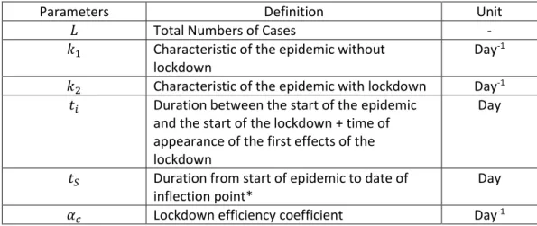
The model is therefore defined by the following six simple parameters:

Parameters Definition Unit

𝐿 Total Numbers of Cases -

𝑘1 Characteristic of the epidemic without

lockdown

Day-1

𝑘2 Characteristic of the epidemic with lockdown Day-1

𝑡𝑖 Duration between the start of the epidemic

and the start of the lockdown + time of appearance of the first effects of the lockdown

Day

𝑡𝑆 Duration from start of epidemic to date of

inflection point*

Day

𝛼𝑐 Lockdown efficiency coefficient Day-1

Table 1: List and definition of the model parameters. * Note that the inflection point of the sigmoid corresponds to the maximum value of its derivative, which is often called "peak of the epidemic".

4- Machine Learning identification algorithm

To obtain the parameters of the model by supervised machine learning, a python code was developed using gradient descents conventionally used in machine learning. In our case, the Levenberg-Marquardt algorithm [19], [20], was chosen to optimize the mean squared error function.

The learning datasets for each country have been compiled using official European information from the European Center for Disease Prevention and Control or ECDC [21]. Considering the small amount of data, it was not possible to build a test data set.

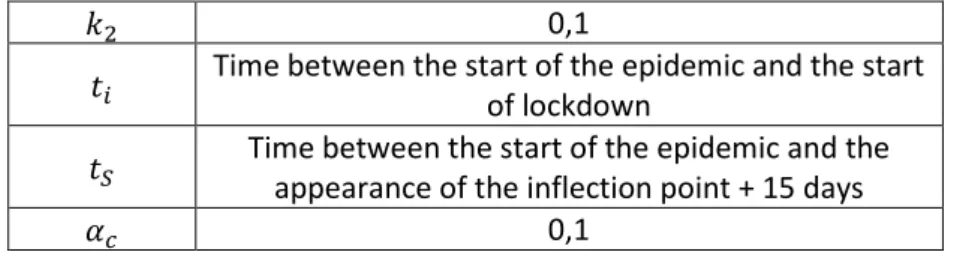
To achieve the learning optimizations for each country, the following initial values have been set:

Parameters Input value in the algorithm 𝐿 0,0031 x Population of the country

𝑘2 0,1

𝑡𝑖 Time between the start of the epidemic and the start _{of lockdown}

𝑡𝑆 Time between the start of the epidemic and the _{appearance of the inflection point + 15 days}

𝛼𝑐 0,1

Table 2: input values of the model parameters, i.e. before supervised learning

These values have been chosen through data analysis to be consistent with our model and the available experimental data.

For 𝐿, 𝑘1, 𝑘2, 𝑡𝑖, 𝑡𝑆, 𝛼𝑐, the input values influences the speed of the convergence of the algorithm and

also ensure the bypassing of local minima:

𝐿 : the input value in the algorithm for the total number of people reached by Covid-19 was chosen to be 0.31% of the total population, following several data analysis.

𝑘1, 𝑘2: their input values are linked to the analysis of the evolution of the epidemic as well as the

analysis of experimental data.

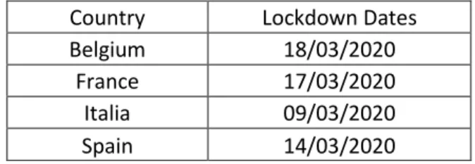
𝑡𝑖 : the start dates of containment of the targeted countries are obviously available on government

websites. They are recalled in Table 3. 10 days are added on those values, to take into account, the needed delay to see the results of the lockdown. This duration, like the other parameters, is optimized by the algorithm.

𝑡𝑆 : the initial value for the inflection date 𝑡𝑆 is chosen lockdown so 𝑡𝑆 is greater than the lockdown

date. 15 days were added on top of that after careful data analysis.

𝛼𝑐 : the initial value was also set after data analysis and after the analysis of simulation curves.

Note that the total population of each country is also provided by the ECDC [21], this information is reported to be from the World Bank Group. https://www.worldbank.org/

Country Lockdown Dates

Belgium 18/03/2020

France 17/03/2020

Italia 09/03/2020

Spain 14/03/2020

Table 3: used in the COVID-19 epidemic

5- Results 5.1- The Data

We took data from a single, reliable official source so that it could be compared across countries [21]. It is obvious that regarding the detection of cases of infected persons, these data are highly dependent on the number of tests carried out and the identification protocols. In addition, it is regularly the case that the data is corrected later following updates. The figures used for Belgium, France, Italy, and Spain are shown in the figures: Fig.1, Fig2, Fig.3 and Fig.4. We can see that the raw data is unsurprisingly very noisy. We will not comment here on the roots of this fact. To increase the ability of the algorithm to quickly converge on a solution, we smoothed the raw data over several days (3 days, 5 days, 7 days). So, for a smoothing over three days, we have: 𝐶𝑖(𝑙𝑖𝑠𝑠é) =

1

3(𝐶𝑖−1+ 𝐶𝑖+ 𝐶𝑖+1). To minimize the noise

effects and obtain the best possible convergence, we decided to use only the values smoothed over 7 days. The last data used dates from April 21, 2020. The smoothing over 7 days implies that the last valid dates for modeling correspond to April 18, 2020. We see on the following figures the raw data and the smoothed data for each country.

Figure 1: Raw data and smoothed data over 7 days of the number of detected cases of COVID-19 in Belgium in 2020 according to [21]

Figure 2: Raw data and smoothed data over 7 days of the number of detected cases of COVID-19 in France in 2020 according to [21] 0 500 1 000 1 500 2 000 2 500 3 000 29/2 10/3 20/3 30/3 9/4 19/4 29/4 N u m b e r o f c ases Date

Belgium : Raw data vs. Smoothed data

Raw data Smoothed data - 21/04 0 1 000 2 000 3 000 4 000 5 000 6 000 7 000 8 000 19/2 29/2 10/3 20/3 30/3 9/4 19/4 29/4 N u m b e r o f c ases Date

France : Raw data vs. Smoothed data

Raw data

Figure 3: Raw data and smoothed data over 7 days of the number of detected cases of COVID-19 in Italy in 2020 according to [21]

Figure 4: Raw data and smoothed data over 7 days of the number of detected cases of COVID-19 in Spain in 2020 according to [21]

5.2- Comparison of the basic functions of the model by country 0 1 000 2 000 3 000 4 000 5 000 6 000 7 000 19/2 29/2 10/3 20/3 30/3 9/4 19/4 29/4 N u m b e r o f c ases Date

Italy : Raw data vs. Smoothed data

Raw data Smoothed data - 21/04 0 1 000 2 000 3 000 4 000 5 000 6 000 7 000 8 000 9 000 10 000 19/2 29/2 10/3 20/3 30/3 9/4 19/4 29/4 N u m b e r o f c ases Date

Spain : Raw data vs. Smoothed data

Raw data

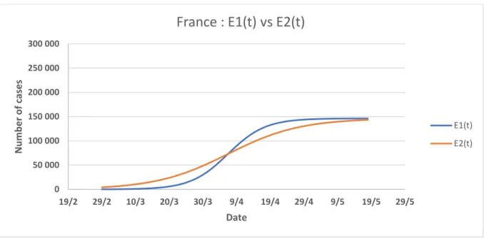
We see in the figures (Fig. 5, Fig. 6, Fig. 7, and Fig. 8) the comparisons of the graphs of the two epidemic functions 𝐸1(𝑡) and 𝐸2(𝑡) which frame the behavior of the epidemic between its standard evolution and its evolution with a lockdown from the start. A marked difference between these two graphs indicates a more significant effect of the lockdown. We could relate it to the efficiency of this lockdown in the considered territory.

Figure 5: Graph of functions 𝐸1(𝑡) and 𝐸2(𝑡) for Belgium, E1 describing the epidemic without a lockdown, E2 with a lockdown from the start.

0 50 000 100 000 150 000 200 000 250 000 300 000 29/2 10/3 20/3 30/3 9/4 19/4 29/4 9/5 19/5 29/5 N u m b e r o f c ases Date

Belgium : E1(t) vs E2(t)

E1(t) E2(t)

Figure 6: Graph of functions 𝐸1(𝑡) and 𝐸2(𝑡) for France, E1 describing the epidemic without a lockdown (in blue), E2 with a lockdown from the start (in red).

Figure 7: Graph of functions 𝐸1(𝑡) and 𝐸2(𝑡) for Italy, E1 describing the epidemic without a lockdown (in blue), E2 with a lockdown from the start (in red).

0 50 000 100 000 150 000 200 000 250 000 300 000 19/2 29/2 10/3 20/3 30/3 9/4 19/4 29/4 9/5 19/5 29/5 N u m b e r o f c ases Date

France : E1(t) vs E2(t)

E1(t) E2(t) 0 50 000 100 000 150 000 200 000 250 000 300 000 19/2 29/2 10/3 20/3 30/3 9/4 19/4 29/4 9/5 19/5 29/5 N u m b e r o f c ases Date

Italy : E1(t) vs E2(t)

E1(t) E2(t)

Figure 8: Graph of functions 𝐸1(𝑡) and 𝐸2(𝑡) for Spain, E1 describing the epidemic without a lockdown (in blue), E2 with a lockdown from the start (in red).

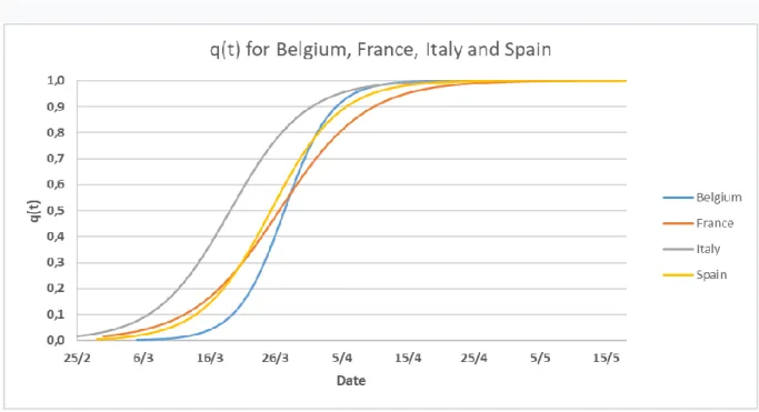
The transition from the function 𝐸1(𝑡) to the function 𝐸2(𝑡) is done by the function 𝑞(𝑡) (Fig. 9). q(t) has been created to be a smoothed Heaviside step like function. The intensity of the slope is causally linked to the efficiency of the lockdown effect as the slope depends of the parameter 𝛼𝑐.

Figure 9: Comparison of the functions q(t) for Belgium, France, Italy, and Spain. The parameters were optimized by machine learning

0 50 000 100 000 150 000 200 000 250 000 300 000 19/2 29/2 10/3 20/3 30/3 9/4 19/4 29/4 9/5 19/5 29/5 N u m b e r o f c ases Date

Spain : E1(t) vs E2(t)

E1(t) E2(t)

5.3- Simulation results for past and current data

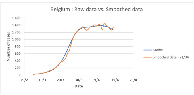
After the machine learning optimization of the parameters, the basic functions have been presented for each country, let us now compare the smoothed data and the model - figures (Fig. 10, Fig. 11, Fig. 12 and Fig. 13)

Figure 10: Comparison between the smoothed data of the number of detected cases of COVID-19 in Belgium and our model

0 200 400 600 800 1 000 1 200 1 400 1 600 29/2 10/3 20/3 30/3 9/4 19/4 29/4 N u m b e r o f c ases Date

Belgium : Raw data vs. Smoothed data

Model

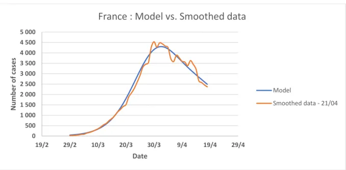
Figure 11: Comparison between the smoothed data of the number of detected cases of COVID-19 in France and our model

Figure 12: Comparison between the smoothed data of the number of detected cases of COVID-19 in Italy and our model

0 500 1 000 1 500 2 000 2 500 3 000 3 500 4 000 4 500 5 000 19/2 29/2 10/3 20/3 30/3 9/4 19/4 29/4 N u m b e r o f c ases Date

France : Model vs. Smoothed data

Model Smoothed data - 21/04 0 1 000 2 000 3 000 4 000 5 000 6 000 19/2 29/2 10/3 20/3 30/3 9/4 19/4 29/4 N u m b e r o f c ases Date

Italy: Model vs. Smoothed data

Model

Figure 13: Comparison between the smoothed data of the number of detected cases of COVID-19 in Spain and our model

5.4- Model predictions

So far, we presented the results up to the date of April 18th_{, i.e. up to the available data with which we}

trained the model. Obviously, one the main question is the quality of the predictions beyond this date. We present the results up to the 18th _{of May in the following figures (Fig. 14, Fig. 15, Fig. 16, and Fig.}

17). Therefore, the reader can observe that the model is based on data available up to the 21th of April (i.e. 18th _{of April once smoothed), we also draw the available data at the time of the publication, that}

is to say up to the 3rd _{of May (i.e. 30}th _{of April once smoothed). This allow the reader to assess the}

quality of the prediction. 0 1 000 2 000 3 000 4 000 5 000 6 000 7 000 8 000 9 000 19/2 29/2 10/3 20/3 30/3 9/4 19/4 29/4 N u m b e r o f c ases Date

Spain : Model vs. Smoothed data

Model

Figure 14:

Comparison between the smoothed data of the number of detected cases of COVID-19 in Belgium (orange : smoothed data available up to the 18st _{of April and used for the model identification, green}

: up to the 30th _{of April) and our model (blue curve) based on the smoothed data of the 18}th _{of April}

Figure 15: Comparison between the smoothed data of the number of detected cases of COVID-19 in France (orange : smoothed data available up to the 18st _{of April and used for the model}

0 200 400 600 800 1 000 1 200 1 400 1 600 19/2 10/3 30/3 19/4 9/5 29/5 N u m b e r o f c ases Date

Belgium : Model vs. Smoothed Data

Model Smoothed data - 21/04 Smoothed data - 03/05 0 500 1 000 1 500 2 000 2 500 3 000 3 500 4 000 4 500 5 000 19/2 10/3 30/3 19/4 9/5 29/5 N u m b e r o f c ases Date

France : Model vs. Smoothed data

Model

Smoothed data - 21/04 Smoothed data - 03/05

identification, green : up to the 30th _{of April) and our model (blue curve) based on the smoothed}

data of the 18th _{of April}

Figure 16: Comparison between the smoothed data of the number of detected cases of COVID-19 in Italy (orange : smoothed data available up to the 18st _{of April and used for the model identification,}

green : up to the 30th _{of April) and our model (blue curve) based on the smoothed data of the 18}th _of

April 0 1 000 2 000 3 000 4 000 5 000 6 000 19/2 10/3 30/3 19/4 9/5 29/5 N u m b e r o f c ases Date

Italy : Model vs. Smoothed data

Model

Smoothed data - 21/04 Smoothed data - 03/05

Figure 17: Comparison between the smoothed data of the number of detected cases of COVID-19 in Spain (orange : smoothed data available up to the 18st _{of April and used for the model identification,}

green : up to the 30th _{of April) and our model (blue curve) based on the smoothed data of the 18}th _of

April. As discussed later, the data quality for Spain seems debatable since on the new dataset (up to the 30th _{of April), the raw data has been changed from the 15}th _{of April with variation up to 160%, even}

stranger the number of cases on the 19th _{of April is negative (-1 400 cases).}

The reader will find below the corresponding value of the optimized parameters for each targeted country. Interestingly, those values are close for all countries, except for the total number of cases L, which obviously relies on country population.

Final Value 𝒕𝒊 𝜶𝒄 𝑳 𝒌𝟐 𝒕𝑺 𝒌𝟏 Belgium 22,31 0,140 56271 0,098 38,23 0,158 France 26,53 0,076 146277 0,093 37,47 0,181 Italy 23,12 0,089 247302 0,063 39,95 0,174 Spain 26,27 0,096 265181 0,074 38,53 0,250 Error 𝒕𝒊 𝜶𝒄 𝑳 𝒌𝟐 𝒕𝑺 𝒌𝟏 Belgium 0,22 0,01 2089 0,00 0,77 0,00 France 1,26 0,01 11025 0,01 1,39 0,01 0 1 000 2 000 3 000 4 000 5 000 6 000 7 000 8 000 9 000 19/2 10/3 30/3 19/4 9/5 29/5 N u m b e r o f c ases Date

Spain : Model vs. Smoothed data

Model

Smoothed data - 21/04 Smoothed data - 03/05

Italy 0,27 0,00 10356 0,00 1,22 0,01

Spain 0,78 0,00 17900 0,01 1,51 0,02

Table 4: Final values of the model parameters for the four countries, and analysis of the corresponding errors (standard deviation error) - 𝑡𝑖 and 𝑡𝑆 in days.

6- Discussion

We see that a simple macroscopic modeling of the Covid-19 epidemic in 2020, built with only two basic functions which permit to consider lockdown and its effects, allows to correctly model the evolution of the cases of people infected by the virus until the dates for which data are available. Simulation of other characteristics of the epidemic, such as the follow-up of hospitalizations or resuscitation, have also been carried out and will be published later [16]. They use the same model and the same optimization algorithm. For the forecasts, they are always to be taken with caution because on the one hand, unexpected events having biological, human causes or of management of the epidemic can occur which modify the form of it in a significant way, on the other hand the assumptions used may seem too summary to assign a level of probability to them. In peculiarly, the unlockdown time can be considered as a new behavior for a given population and modeled with a new elementary function in addition to the two functions used. This unlockdown time is not considered in the simulations. The results are however interesting and show how a learning algorithm can allow a simple model to correspond well to the macroscopic effects of the epidemic.

It will also be noted that the inflection point of the 𝑡𝑆 sigmoid occurs on average 38.65 days (from 37.47 to 39.95) after the start of the epidemic (Table 4) for the four countries. This means that as of this date, half of the people who will be affected by the epidemic have been infected. Analysis of the values of 𝑡𝑖 (duration entered at the start of the epidemic and the date of lockdown + duration of appearance of the first effects of lockdown) shows that the duration of appearance of the effects of

lockdown is very similar for the four countries , of the order of 10.30 days (between 9.53 for France and 11.27 for Spain). It should also be noted that the number of infected cases is half lower in France than in Italy and then in Spain.

The parameters 𝛼𝑐 are associated to the velocity of changing of behavior after the lockdown. France, Italy, and Spain, with 𝛼𝑐 between 0,076 and 0,096, have similar reactions for this evolution. By the way, to appreciate the step between the two behaviors, we must analyze the step between 𝑘1 and 𝑘2 for each country. The ratio 𝑘1⁄𝑘2 represents the intensity of this change. In that case, Belgium appears to have the smallest change of behavior with a ratio of 1,62. France a ratio of 1,92 is better. Italy has a high ratio of 2,76 and Spain has strongly changed its behavior with a ratio of 3,36.

It interesting to remember that the equation of the elementary basic functions 𝐸𝑘(𝑡) of the epidemic, given by the equation (2), or its initial form given in equation (1), are the solution of a elementary differential equation detailed in 2.1. This differential equation is solved for the boundary condition 𝑦(0) = 𝑦0. The boundary condition 𝑦0 characterizes the number of cases at time 𝑡0. We show in the table 5 the values of 𝑦0 given by the raw data and the smoothed data. They can be compared with the values of 𝑦0 obtained by the modeling after the machine learning process. The differences of these values for raw and smoothed data are the intensity of the noise associated to these data. On the opposite, the differences between the values of 𝑦0 for the data and the modeling are interesting. It shows that the number of cases at time 𝑡0 were strongly underestimated by a factor 5 in Italy and in Belgium, and by a factor 10 for France and Spain. The more precise measurement of these boundary conditions at 𝑡0 could have helped to better appreciate the intensity of this epidemic in a short time.

Country 𝑦0 Raw Data (Sum of the new cases from 𝑡 = −3 to 𝑡 = 0)

𝑦0 Smoothed Data (Value of new cases at 𝑡 = 0)

𝑦0 given by the Model

France 45 24 237

Italy 226 92 524

Spain 23 12 109

Table 5 : Values of the number of cases 𝑦0 at 𝑡0 measured with the raw and smoothed data, comparing to the number of cases 𝑦0 at 𝑡0 given by the model.

Note the extremely high value of 𝑦0 for Belgium compared with the number of the inhabitants of this country, six times lower than the three other countries.

The coefficients 𝑅2 of the model are given in the table below and by country, with smoothed and non-smoothed data. We see that the simulation is particularly good for non-smoothed data. For raw data, the case of France is special given the positive data jumps that were recorded on certain days for administrative reasons. For Spain, despite of a good 𝑅2 coefficient which show a good correlation between the data and the model, the official data given by this country after the identification of the model have changed strongly after the 15th _{of April. Then there is no peculiar significance on the}

analysis of this variation.

Country Smoothed Data Row Data – 18th April

Belgium 0,993 0,733

France 0,986 0,648

Italy 0,996 0,928

Spain 0,995 0,928

Table 5: 𝑅2 coefficient of quality of simulations compared to raw data and smoothed data.

Therefore, this global modeling of the COVID-19 epidemic seems to be understandable as a sum of only two different elementary basis functions including the effects of the lockdown, and the

development of such analysis will probably permit to analyze the specific behavior of population, in complement of the classical approaches by micro-macro analysis.

7- Conclusion

We have created a particularly simple virus-centric model of the Covid-19 epidemic, based on a decomposition in generic basic functions adaptable to all countries and to all the characteristic criteria of its development. Using a simple machine learning process, we show that only two basic elementary functions were sufficient to simulate the epidemic evolution for four European countries applying a lockdown, with accuracy. The results permit to quantify the difference of behavior before and after the lockdown for these countries as well as the velocity of change and the intensity of change. We focused here on the model's ability to simulate the numbers of new cases reported in the Covid-19 epidemic over time. However, this model could be used for modeling hospitalizations, intensive care, and death. The prediction of a unlockdown effects should be also possible with this model, by adding a third elementary basic function describing the specific behavior of population after this event. The presented simulations are relevant and clearly show the effects of the various lockdowns carried out. The analysis of basic functions used in this decomposition could in any case allow us to have a macroscopic analysis of how the lockdowns were respected. Other characteristics and simulations of the 2020 SARS CoV 2 epidemic for other countries will be given in the part 2 of the paper [22].

8- References

[1] T.L. Wiemken, R.R. Kelley, Machine learning in epidemiology and health outcomes research, Annual Review of Public Health, Vol.41, April 2020, p.21-36

[2] V. Colizza, A. Barrat, M. Barthelemy, A. Vespignani, The modeling of global epidemics: Stochastic dynamics and predictability, Bulletin of Mathematical Biology, Vol.68 (8), December 2006, p.1893-1921

[3] Lin Jia, Kewen Li, Yu Jiang, Xin Guo, Ting Zhao, Prediction and analysis of Coronavirus Disease 2019, 2020, arxiv.org/abs/2003.05447v2

[4] D. Caccavo, Chinese and Italian COVID-19 outbreaks can be correctly described by a modified SIRD model, 2020, https://www.medrxiv.org/content/10.1101/2020.03.19.20039388v2

[5] C. Bayette, M. Monticelli, https://images.math.cnrs.fr/Modelisation-d-une-epidemie-partie-1.html (in french)

[6] J. Moral, A. Trapero, Assessing the Susceptibility of Olive Cultivars to Anthracnose Caused by Colletottrichum acutatum, Plant Disease, Vol. 93, n°10, October 2009, p.1028-1036

[7] Z. Mesha, B. Hau, Effects of bean rust (Uromyces appendiculatus) epidemics on host dynamics of common bean, Plant Pathology, 57, 2008, p.674-686

[8] I.J. Holb et al. Analysis of Summer Epidemic Progress of Apple Scab at Different Apple Production Systems in the Netherlands and Hungary, J. of Phytopathology, Vol. 95, n°9, 2005, p.1001-1020

[9] S.G. Mahiane et al., Improvements in Spectrum’s fit to program data tool, AIDS, Vol. 31 (Suppl 1), 2017, p.S23-S30

[10] J.W. Eaton et al., The Estimation and Projection Package Age-Sex Model and r-hybrid Model: new tools for estimating HIV incidence trends in sub-Saharan Africa, AIDS, Vol. 33, (Suppl 3), 2019, p.S235-S244

[11] F. Chinesta, E. Cueto, PGD-Based Modeling of Materials, Structures and Processes, ESAform Bookseries on Materials Forming, 2014, Springer,

[12] G. Allaire, Shape optimization by the homogenization method, Springer Verlag, New York, 2001

[13] O. Oleinik, A. Shamaev, G. Yosifian, Mathematical Problems in Elasticity and Homogenization Studies in Mathematics and its Application, Vol. 26 Elsevier, Amsterdam, 1992

[14] E. Sanchez-Palencia, Non-Homogeneous Media and Vibration Theory, Springer, Lecture Notes in Physics 129, 1980

[15] P.M. Suquet, Elements of Homogenization for Inelastic Solid Mechanics, Homogenization Techniques for Composite Media, 105, 1987, p.193-278, Springer-Verlag

[16] Y. Rémond, S. Ahzi, M. Baniassadi, H. Garmestani, Applied RVE Reconstruction of Heterogeneous Materials, Wiley-ISTE Ed., 2016

[17] P-F. Verhulst, Notice sur la loi que la population poursuit dans son accroissement, Correspondance

mathématique et physique, no _{10, 1838, p.113-121}

[18] Epidemic Modelling, D.J.Daley, J.Gani, Cambridge University Press, 1999, ISBN 0 521 01467-0

[19] D.W. Marquardt, An algorithm for least-squares estimation of non linear parameters, SIAM J. Appl. Math., Vol. 11, 1963, p.431-441

[20] K. Levenberg, A method for the solution of certain problems in least squares, Quart. Appl. Math., Vol. 2, 1944, p.164-168

[21] https://www.ecdc.europa.eu/en

[22] J.Rémond, Y.Rémond, On a New Virus-centric Epidemic Modeling, Part 2: Simulation of deceased of 2020 SARS CoV 2 in several countries, submitted to Mathematics and Mechanics of Complex System