Image analysis by discrete orthogonal dual Hahn moments

HAL Id: inserm-00189813

https://www.hal.inserm.fr/inserm-00189813

Submitted on 23 Nov 2007

HAL is a multi-disciplinary open access archive for the deposit and dissemination of sci-entific research documents, whether they are pub-lished or not. The documents may come from teaching and research institutions in France or

L’archive ouverte pluridisciplinaire HAL, est destinée au dépôt et à la diffusion de documents scientifiques de niveau recherche, publiés ou non, émanant des établissements d’enseignement et de recherche français ou étrangers, des laboratoires

Image analysis by discrete orthogonal dual Hahn

moments

Hongqing Zhu, Huazhong Shu, Jian Zhou, Limin Luo, Jean-Louis Coatrieux

To cite this version:

Hongqing Zhu, Huazhong Shu, Jian Zhou, Limin Luo, Jean-Louis Coatrieux. Image analysis by discrete orthogonal dual Hahn moments. Pattern Recognition Letters, Elsevier, 2007, 28 (13), pp.1688-1704. �10.1016/j.patrec.2007.04.013�. �inserm-00189813�

Image analysis by discrete orthogonal dual Hahn moments

Hongqing Zhua_{, Huazhong Shu}a, c_{*, Jian Zhou}a_{, Limin Luo}a, c_{, J. L. Coatrieux}b, c

a

_{Laboratory of Image Science and Technology, Department of Computer Science and}

Engineering, Southeast University, 210096 Nanjing, People’s Republic of China

b

_{INSERM U642, Laboratoire Traitement du Signal et de l’Image, Université de Rennes I, 35042}

Rennes, France

c

_{Centre de Recherche en Information Biomédicale Sino-français (CRIBs)}

*

Information about the corresponding author:

Huazhong Shu, Ph. D

Lab. of Image Science and Technology,

Department of Computer Science and Engineering,

Southeast University

210096 Nanjing

People’s Republic of China

Tel: 00-86-25-83794249

Fax: 00-86-25-83794298

Email: [email protected]

HAL author manuscript inserm-00189813, version 1

HAL author manuscript

Abstract

In this paper, we introduce a set of discrete orthogonal functions known as dual Hahn polynomials. The Tchebichef and Krawtchouk polynomials are special cases of dual Hahn polynomials. The dual Hahn polynomials are scaled to ensure the numerical stability, thus creating a set of weighted orthonormal dual Hahn polynomials. They are allowed to define a new type of discrete orthogonal moments. The discrete orthogonality of the proposed dual Hahn moments not only ensures the minimal information redundancy, but also eliminates the need for numerical approximations. The paper also discusses the computational aspects of dual Hahn moments, including the recurrence relation and symmetry properties. Experimental results show that the dual Hahn moments perform better than the Legendre moments, Tchebichef moments, and Krawtchouk moments in terms of image reconstruction capability in both noise-free and noisy conditions. The dual Hahn moment invariants are derived using a linear combination of geometric moments. An example of using the dual Hahn moment invariants as pattern features for a pattern classification application is given.

Keywords: Discrete orthogonal moments; Dual Hahn polynomials; Image reconstruction; Pattern

classification

1. Introduction

Since Hu (1962) introduced moment invariants, moments and functions of moments due to their ability to represent global features of an image have found wide applications in the fields of image processing and pattern recognition such as noisy signal and image reconstruction (Yin et al., 2002; Mukundan et al., 2001b), image indexing (Mandal et al., 1996), robust line fitting (Kiryati et al., 2000), and image recognition (Qing et al., 2004). Among the different types of moments, the Cartesian geometric moments are most extensively used. However, the geometric moments are not orthogonal. The lack of orthogonality leads to a certain degree of information redundancy and causes the recovery of an image from its geometric moments strongly ill-posed. Indeed, the fundamental reason for the ill-posedness of the inverse moment problem is the serious lack of orthogonality of the moment sequence (Talenti, 1987). To surmount this shortcoming, Teague (1980) suggested the use of the continuous orthogonal moments defined in terms of Legendre and Zernike polynomials. Since the Legendre polynomials are orthogonal over the interval [-1, 1], and Zernike polynomials are defined inside the unit circle, the computation of these moments requires a suitable transformation of the image coordinate space and an appropriate approximation of the integrals (Shu et al., 2000; Chong et al., 2003).

The study of classical special functions and in particular the discrete orthogonal polynomials has recently received an increasing interest (Mukundan et al., 2001a; Arvesú et al., 2003; Foupouagnigni and Ronveaux, 2003; Ronveaux et al., 2000). The use of discrete orthogonal polynomials in image analysis was first introduced by Mukundan et al. (2001b) who proposed a set of discrete orthogonal moment functions based on the discrete Tchebichef polynomials. An efficient method for computing the discrete Tchebichef moments was also developed (Mukundan, 2004). Another new set of discrete orthogonal moment functions based on the discrete Krawtchouk polynomials was presented by Yap et al. (2003). It was shown (Mukundan et al., 2001b, Yap et al. 2003) that the discrete orthogonal moments perform better than the conventional continuous orthogonal moments in terms of image representation capability.

The classical orthogonal polynomials can be characterized by the existence of a differential equation. In fact, the classical continuous polynomials (e.g., Hermite, Laguerre, Jacobi, Bessel) satisfy a differential equation of the form (Nikiforov and Uvarov, 1988):

0

)

(

)

(

'

)

(

~

)

(

''

)

(

~

_x

_y

_x

₊

_τ

_x

_y

_x

₊

_λ

_y

_x

₌

σ

(1) where

σ

~ x

(

)

and

τ

~ x

(

)

are polynomials of at most second and first degree, and λ is an appropriate constant. It is possible to expand polynomial solutions of partial differential equations in any basis of classical orthogonal polynomials.

When the differential equation (1) is replaced by a difference equation, we can find the main properties of classical orthogonal polynomials of a discrete variable. Consider the simplest case, when (1) is replaced by the following difference equation

0

)

(

)

(

)

(

)

(

)

(

2

)

(

~

)

(

)

(

)

(

)

(

1

)

(

~

₊

₌

⎥⎦

⎤

⎢⎣

⎡

−

−

+

−

+

+

⎥⎦

⎤

⎢⎣

⎡

−

−

−

−

+

x

y

h

h

x

y

x

y

h

x

y

h

x

y

x

h

h

x

y

x

y

h

x

y

h

x

y

h

x

τ

λ

σ

(2) which approximates (1) on a lattice of constant mesh Δx = h. The classical discrete polynomials such as Charlier, Meixner, Tchebichef, Krawtchouk, and Hahn polynomials are all the polynomial solutions of (2).

After a change of independent variable x = x(s) in (2), we can obtain a further generalization when (1) is replaced by a difference equation on a class of lattices with variable mesh Δx = x(s+h) – x(s) (Nikiforov and Uvarov, 1988). The discrete orthogonal polynomials on the non-uniform lattice are of great importance for applications in quantum integral systems, quantum field theory and statistical physics (Vega, 1989). In recent years, much attention has been paid to the study of this class of polynomials (Koepf and Schmersau, 2001; Kupershmidt, 2003; Álvarez-Nodarse, 2001a,b; Álvarez-Nodarse and Smirnov, 1996; Temme and López, 2000). However, to the best of our knowledge, until now, no discrete orthogonal polynomials defined on a non-uniform lattice have been used in the field of image analysis. In this paper, we address this problem by introducing a new set of discrete orthogonal polynomials, namely the dual Hahn polynomials, which are orthogonal on a non-uniform lattice (quadratic lattices x(s) = s(s + 1)). The dual Hahn polynomials are scaled, to ensure that all the computed moments have equal weights, and are used to define a new type of discrete orthogonal moments known as dual Hahn moments. Similar to Tchebichef and Krawtchouk moments, there is no need for spatial normalization; hence, the error in the computed dual Hahn moments due to discretization does not exist. However, our new moments are more

general because both the Tchebichef and Krawtchouk polynomials are special cases of the dual Hahn polynomials (Nikiforov and Uvarov, 1988). Since the dual Hahn moments contain more parameters (due to the fact that the dual Hahn polynomials are defined on the non-uniform lattice) than the discrete Tchebichef and Krawtchouk moments, these extra parameters give more flexibility in describing the image, the improvement in performance could thus be expected.

It is worth mentioning that although the dual Hahn polynomials are orthogonal on a non-uniform lattice, the discrete dual Hahn moments defined in this paper are still applied to uniform pixel grid image. The difference between the dual Hahn moments and the discrete moments based on the polynomials that are orthogonal on uniform lattice (e.g., discrete Tchebichef moments and Krawtchouk moments) is that the latter is directly defined on the image grid but, for the former, we should introduce an intermediate,

non-uniformlattice,

x

(

s

)

= s

s

(

+

1

)

.

The rest of the paper is organized as follows. In section 2, we introduce the dual Hahn polynomials of a discrete variable. This section also provides the derivation of weighted dual Hahn polynomials and the dual Hahn moments. Section 3 discusses the computational aspects of dual Hahn moments. It is shown how the recurrence formulae and symmetry property of the dual Hahn polynomials can be used to facilitate the moment computation. The dual Hahn moment invariants are also derived in this section. The experimental results are provided and discussed in Section 4. Section 5 concludes the paper.

2. Dual Hahn Moments

2.1. Discrete orthogonal polynomials on the non-uniform lattice

Let us first review some general properties of orthogonal polynomials of a discrete variable on a non-uniform lattice (Nikiforov and Uvarov, 1988; Álvarez-Nodarse and Smirnov, 1996). As previously indicated, the discrete orthogonal polynomials on the non-uniform lattice can be constructed using a variable mesh in (1) when it is replaced by a difference equation. Let

0 ) ( ] ) ( ) ( ) ( ) ( [ 2 )) ( ( ~ ] ) ( ) ( [ ) 2 1 ( )) ( ( ~ _{+ =} ∇ ∇ + + ∇ ∇ − s y s x s y s x s y s x s x s y s x s x τ λ σ Δ Δ Δ Δ (3)

be the second order difference equation of hypergeometric type for some lattice function x(s), where

)

1

(

)

(

)

(

=

−

−

∇

g

s

g

s

g

s

,

Δ

g

(

s

)

=

g

(

s

+

1

)

−

g

(

s

)

(4) denote respectively the backward and forward finite difference quotients.

σ

~ x

(

)

and

τ

~ x

(

)

are polynomials in x(s) of degree at most two and one, respectively, and λ is a constant. It is convenient to rewrite (3) in the following equivalent form (Nikiforov and Uvarov, 1988; Álvarez-Nodarse and Smirnov, 1996) 0 ) ( ] ) ( ) ( )[ ( ] ) ( ) ( [ ) 2 1 ( ) ( + + = ∇ ∇ − s y s x s y s s x s y s x s τ λ σ Δ Δ Δ Δ (5) where

)]

2

1

(

))[

(

(

~

2

1

))

(

(

~

)

(

s

=

σ

x

s

−

τ

x

s

Δ

x

s

−

σ

(6)

))

(

(

~

)

(

s

τ

x

s

τ

=

(7) The polynomial solutions of equation (5), denoted by

y

_n

(

x

(

s

))

≡

P

_n

(

s

)

, are uniquely determined, up to a normalizing factor Bn, by the difference analogue of the Rodrigues formula (Nikiforov and Uvarov,

1988)

)]

(

[

)

(

)

(

( )

_s

s

B

s

P

n _n n n n

=

_ρ

∇

ρ

,

[

(

)]

)

(

)

(

)

(

)]

(

[

1 1 ) (

_s

s

x

s

x

s

x

s

_n n n n n n

ρ

_∇

ρ

∇

∇

∇

⋅⋅

⋅

∇

∇

=

∇

− (8) where

)

2

(

)

(

s

x

s

n

x

_n

=

+

,

∏

(9) =

+

+

=

n k n

s

n

s

s

k

1

)

(

)

(

)

(

ρ

σ

ρ

It is known that for some special kind of lattices, solutions of (5) are orthogonal polynomials of a discrete variable, i.e., they satisfy the following orthogonality property (Nikiforov and Uvarov, 1988)

1

_)]

2

2

1

(

)[

(

)

(

)

(

_{m nm n} b a s n

s

P

s

s

x

s

d

P

ρ

Δ

−

=

δ

∑

− = (10)

where denotes the square of the norm of the corresponding orthogonal polynomials, and ρ(s) is a nonnegative function (weighting function), i.e.,

2 n

d

)]

0

2

1

(

)[

(

s

Δ s

x

−

>

ρ

, a ≤ s ≤ b – 1 (11)

supported in a countable set of the real line (a, b) and such that

)

(

)

(

)]

(

)

(

[

)

2

1

(

x

x

x

x

s

x

ρ

τ

ρ

σ

=

−

Δ

Δ

(12)

Some important discrete orthogonal polynomials on the non-uniform lattice are listed in Table 1. Among them, the dual Hahn polynomials and Racah polynomials are relatively simple in terms of the lattice form and weighting function, moreover, both polynomials have a finite domain of definition that is suited for square images of size N×N pixels. We choose here the dual Hahn polynomials to define a new type of moments. The Racah polynomials have already been used by the authors in another paper (Zhu et al, 2007). A comparison of these two moments is given in Table 2.

2.2. Dual Hahn polynomials

The classical dual Hahn polynomials , n = 0, 1, …, N–1, defined on a non-uniform lattice x(s) = s(s+1), are solutions of (5) corresponding to (Nikiforov and Uvarov, 1988)

)

,

,

(

) (

_s

_a

_b

w

c n n s x c b a bc ac ab s c s b s a s s = − − − + − + − = − + − =

λ

τ

σ

) ( 1 ) ( ) )( )( ( ) ( (13)

and the weighting function ρ(s) is given by

) 1 ( ) 1 ( ) ( ) 1 ( ) 1 ( ) 1 ( ) ( + − Γ + + Γ − Γ + − Γ + + Γ + + Γ = c s s b s b a s s c s a s

ρ

(14)

where the parameters a, b and c are restricted to

N

a

b

a

c

b

a

<

<

+

=

+

<

−

1

/

2

,

1

,

₍₁₅₎

Note that if the uniform lattice, i.e., x(s) = s, is used in (5), and the parameters a, b, and c are defined as 2

/ ) (α+β =

a , b = a + N, c=(β−α)/2, the dual Hahn polynomials become the Hahn polynomials (Nikiforov and Uvarov, 1988). Setting α = 0 and β = 0, the Hahn polynomials reduce to the Tchebichef polynomials. If we take β = pt and α = (1–p)t in the Hahn polynomials and let t → ∞, we obtain the Krawtchouk polynomials Kn(x; p, N) (Koekoek and Swarttouw, 1998).

)

,

(

) , (

_x

_N

h

_nαβ

The n-th order dual Hahn polynomials are defined as (Álvarez-Nodarse and Smirnov, 1996)

( , , 1; 1, 1;1) ! ) 1 ( ) 1 ( ) , , ( _{3 2} ) ( ₌ − + + + _{F −n a−s a+s+ a−b+ a+c+} n c a b a b a s wc n n n n = 0, 1, …, N – 1, s = a, a + 1, …, b – 1, (16) where (u)k is the Pochhammer symbol defined as

) ( ) ( ) 1 ( ) 1 ( ) ( u k u k u u u u _k Γ + Γ = − + + = _L (17) and ₃F₂(⋅) is the generalized hypergeometric function given by

! ) ( ) ( ) ( ) ( ) ( ) ; , ; , , ( 0 1 2 3 2 1 2 1 3 2 1 2 3 k z b b a a a z b b a a a F k k k k k k k

∑

∞ = = (18) The dual Hahn polynomials satisfy the following orthogonality property

2 1 ) ( ) (

_)]

2

1

(

)[

(

)

,

,

(

)

,

,

(

_{nm n} b a s c m c n

s

a

b

w

s

a

b

s

x

s

d

w

ρ

Δ

−

=

δ

∑

− = , n, m = 0, 1, …, N – 1 (19)

where the weighting function ρ(s) is given by (14) and

) ( )! 1 ( ! ) 1 ( 2 n c b n a b n n c a d_n − − Γ − − − + + + Γ = , n = 0, 1, …, N – 1 (20) The set of dual Hahn polynomials is not suitable for defining the moments because the range of values of the polynomials expands rapidly with the order. To surmount this shortcoming, we introduce the weighted dual Hahn polynomials in the following subsection.

2.3. Weighted dual Hahn polynomials

To avoid numerical instability in polynomial computation, the dual Hahn polynomials are scaled by utilizing the square norm and the weighting function. The set of the weighted dual Hahn polynomials is defined as )] 2 1 ( [ ) ( ) , , ( ) , , ( ˆ( ) ₌ ( ) _{2 Δx s−} d s b a s w b a s w n c n c n

ρ

n = 0, 1, …, N – 1 (21)

In this case, the orthogonality condition given by (19) becomes

nm b a s c m c n

s

a

b

w

s

a

b

w

=

δ

∑

− = 1 ) ( ) (

₍

_,

_,

₎

_ˆ

₍

_,

_,

₎

ˆ

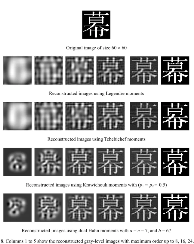
n, m = 0, 1, …, N – 1 (22)

The values of the weighted dual Hahn polynomials are thus confined within the range of [-1, 1]. Fig. 1 shows the plots for the first few orders of the weighted dual Hahn polynomials with the parameters a = c = 0 and b = N = 40.

2.4. Dual Hahn moments

The dual Hahn moments are a set of moments formed by using the weighted dual Hahn polynomials. Given a uniform pixel lattices image f(s, t) with size N × N, the (n + m)-th order dual Hahn moment is defined as

)

,

(

)

,

,

(

ˆ

)

,

,

(

ˆ

1 1 ) ( ) (

_s

_a

_b

_w

_t

_a

_b

_f

_s

_t

w

W

b a s b a t c m c n nm

∑∑

− = − =

=

n, m = 0, 1, …, N – 1 (23)

The orthogonality property of the dual Hahn polynomials helps in expressing the image intensity function f(s, t) in terms of its dual Hahn moments. The reconstructed image can be obtained by using the following inverse moment transform.

∑∑

, s, t = a, a + 1, …, b – 1 (24) − = − = = 1 0 1 0 ) ( ) ( _{( , , )ˆ ( , , )} ˆ ) , ( N n N m c m c n nmw s a b w t a b W t s f

In (24), s and t represent horizontal and vertical directions of reconstructed image with uniform pixel grid. If only the dual Hahn moments of order up to M are used, (24) is approximated by

∑∑

= =

=

M n M m c m c n nm

w

s

a

b

w

t

a

b

W

t

s

f

0 0 ) ( ) (

₍

_,

_,

₎

_ˆ

₍

_,

_,

₎

ˆ

)

,

(

(25)

3. Computational Aspects of Dual Hahn Moments

In this section, we discuss the computational aspects of dual Hahn moments. We present some properties of dual Hahn polynomials and show how they can be used to facilitate the computation of moments.

3.1. Recurrence relation with respect to n

In order to decrease the computational cost in the calculation of moments, the recurrence relation can be used to avoid the overflowing for mathematical functions like the hypergeometric and gamma

functions. The weighted dual Hahn polynomials obey the following recurrence relation (the derivation of the relation is given in Appendix A)

) , , ( ˆ ) , , ( ˆ ) , , ( ˆ ( ) 2 2 ) ( 1 1 ) ( _{w s a b} d d B b a s w d d A b a s w c n n n c n n n c n = − − + − − (26) where

]

)

1

(

2

)

1

2

)(

1

(

)

1

(

[

1

₊

₋

₊

₋

₋

₋

₋

₋

₋

₊

₋

2

=

s

s

ab

ac

bc

b

a

c

n

n

n

A

₍₂₇₎ ) 1 )( 1 )( 1 ( 1 _{+ + − − − + − − +} − = a c n b a n b c n n B (28) with )] 2 1 ( [ ) ( ) , , ( ˆ ₂ 0 ) ( 0 = Δx s− d s b a s wc

ρ

(29) )] 2 1 ( [ ) ( ) 2 / 1 ( ) 2 / 1 ( ) 1 ( ) ( ) ( 1 ) , , ( ˆ ₂ 1 1 1 ) ( 1 _{+ − −} Δ − − − − = x s d s s x s x s s s b a s wc

ρ

ρ

ρ

ρ

(30)

Equation (26) is used to compute the values of the weighted dual Hahn polynomials. The algorithm for computing the dual Hahn polynomial values is shown in Fig. 2. Fig. 3 shows the reconstruction algorithm based on equation (24).

) , , ( ˆ( ) _{s a b} wc n

3.2. Recurrence relation with respect to s

The recurrence relation of discrete dual Hahn polynomials with respect to s is as follows (The detailed derivation is given in Appendix B):

) , , 2 ( )] 1 ( ) 1 2 ( ) 1 ( )[ 1 ( ) 1 ( ) , , 1 ( )] 1 ( ) 1 2 ( ) 1 ( )[ 1 ( )] 1 ( 2 ) 1 ( ) 1 ( ) 1 ( )[ 1 2 ( ) , , ( ) ( ) ( ) ( b a s w s s s s s s b a s w s s s s s s s s s s b a s w c n c n c n − − − + − − − ⋅ − − − − + − − − ⋅ − − − + − − =

τ

σ

σ

τ

σ

λ

τ

σ

(31)

To obtain the values for s = 0 and s = 1, we derive defined by (8) for dual Hahn polynomials as follows (Álvarez-Nodarse, 2001a)

)]

(

[

) (

_s

n n n

ρ

∇

) ( ) 2 / ) 1 ( ( ) 2 / 1 ( )! ( ! ! ) 1 ( )] ( [ 0 0 ) ( _{s l} l m s x l s x l n l n s _{n n} m n n n l l n n n − − + − ∇ + − ∇ × − − = ∇

∏

∑

= =

ρ

ρ

(32)

Using (32) andx(s)= ss( +1), we have

! ) 0 ( ) 0 ( ) 1 ( 1 ) 2 1 ( ) 2 1 ( ) 0 ( ) 2 1 ( ) 2 1 ( ) 0 ( 0 0 0 ) ( n m n n m n x n x m x x n n n m n m n n m n n n n n ρ ρ ρ ρ = ⋅ + − + = + − ∇ + ∇ = ⋅ − − ∇ ∇ = ∇

∏

∏

∏

= = = (33) ) 0 ( )! 2 ( ) 1 ( ) 1 ( )! 2 ( 2 ) 0 ( ) 2 ( ) 1 ( ) 1 ( ) 3 ( 3 ) 1 ( 0 0 ) ( n n n n m n n m n n n n n n n m n n n m n n ρ ρ ρ ρ ρ ⋅ + + − ⋅ + = ⋅ − + + − ⋅ − + + = ∇

∏

∏

= = (34)

we deduce from (8), (33) and (34) that

n n n c n

a

c

b

n

n

b

a

w

(

1

)

(

1

)

(

)

)

!

(

1

)

,

,

0

(

₂ ) (

₌

₋

₊

₊

₋

₍₃₅₎ ) , , 0 ( ] 2 ) 1 ( ) 0 ( ) 1 ( [ ) 1 ( ) 0 ( ) 1 )( 2 ( 2 ) , , 1 ( ( ) ) ( n n _{w a b} n n b a w c n n n c n + − + + =

ρ

ρ

ρ

ρ

(36) ) 1 ( ) 1 ( ) ( ) 1 ( ) 1 ( ) 1 ( ) ( + − Γ + + Γ − − Γ + − Γ + + + Γ + + + Γ = c s s b n s b a s n s c n s a s n

ρ

(37)

Similarly, we can obtain the recurrence relation for the weighted dual Hahn polynomials with respect to s

) , , 2 ( ˆ ) 3 2 )( 2 ( )] 2 1 ( )[ ( )] 1 ( ) 1 2 ( ) 1 ( )[ 1 ( ) 1 ( ) , , 1 ( ˆ ) 1 2 )( 1 ( )] 2 1 ( )[ ( )] 1 ( ) 1 2 ( ) 1 ( )[ 1 ( )] 1 ( 2 ) 1 ( ) 1 ( ) 1 ( )[ 1 2 ( ) , , ( ˆ ) ( ) ( ) ( b a s w s s s x s s s s s s s b a s w s s s x s s s s s s s s s s s b a s w c n c n c n − − − − Δ − − + − − − ⋅ − − − − − Δ − − + − − − ⋅ − − − + − − =

ρ

ρ

τ

σ

σ

ρ

ρ

τ

σ

λ

τ

σ

n = 0, 1, …, N – 1, s = 2, 3, …, b – 1 (38) with

) , , 0 ( ˆ ) )( )( ( 1 ) 0 ( ) ( ) 1 ( ) 1 ( ) ! ( 1 ) , , 0 ( ˆ ( ) 1 1 2 2 2 ) ( _{w a b} d d n b n c n a n d n b c a n b a w c n n n n n n n c n =− + + − =− + + − − −

ρ

(39) ) , , 0 ( ˆ ) 0 ( ) 1 ( 3 2 ) 1 ( ) 0 ( ) 1 ( ) 1 ( ) 0 ( ) 1 )( 2 ( 2 ) , , 1 ( ˆ( ) n n _w( ) _{a b} n n b a w c n n n c n

_ρ

ρ

ρ

ρ

ρ

ρ

⎥ ⎦ ⎤ ⎢ ⎣ ⎡ ₋ + + + = (40)

Equations (38), (39) and (40) can be used to effectively calculate the weighted dual Hahn polynomial values.

3.3. Symmetry property

The symmetry property can be used to reduce the time required for computing the dual Hahn moments. The weighted dual Hahn polynomials have the symmetry property with respect to n

)

,

,

(

ˆ

)

1

(

)

,

,

(

ˆ

( ) 1 ) (

_s

_a

_b

_w

_s

_a

_b

w

c n N s c n

=

−

−− (41) The above relation shows that only the values of the dual Hahn polynomials up to order n = N/2 – 1 need to be calculated, thus the computational cost can be reduced.

The symmetry property is also useful in minimizing the memory requirements for storing the dual Hahn polynomial values. In fact, equation (23) can be rewritten as

(42)

⎪

⎪

⎪

⎪

⎪

⎪

⎪

⎩

⎪

⎪

⎪

⎪

⎪

⎪

⎪

⎨

⎧

> > ∑ ∑ − > < ∑ ∑ − < > ∑ ∑ − < < ∑ ∑ = − = − = −− −− + − = − = −− − = − = −− − = − = 2 / and 2 / if ) , ( ) , , ( ˆ ) , , ( ˆ ) 1 ( 2 / and 2 / if ) , ( ) , , ( ˆ ) , , ( ˆ ) 1 ( 2 / and 2 / if ) , ( ) , , ( ˆ ) , , ( ˆ ) 1 ( 2 / and 2 / if ) , ( ) , , ( ˆ ) , , ( ˆ 1 1 _{( )} 1 ) ( 1 1 1 _{( )} 1 ) ( 1 1 _{( ) ( )} 1 1 1 _{( ) ( )} N m N n t s f b a t w b a s w N m N n t s f b a t w b a s w N m N n t s f b a t w b a s w N m N n t s f b a t w b a s w W b a s b a t c m N c n N t s b a s b a t c m N c n t b a s b a t c m c n N s b a s b a t c m c n nm

Using (41), the inverse transformation (24) can be modified as

(43)

[

nm s N nm t nN m s t N nN m

]

c m N n N m c n W W W W b a t w b a s w t s f − − − − + − − − − − = − = − + − + − + × =

∑ ∑

1 , 1 1 , , 1 ) ( 1 2 / 0 1 2 / 0 ) ( ) 1 ( ) 1 ( ) 1 ( ) , , ( ˆ ) , , ( ˆ ) , (

where f(s, t) represents image intensity with uniform pixel grid. Such decomposition permits decreasing the computational complexity in the reconstruction process. In fact, the number of multiplication required in (43) is N2/4 assuming that all the polynomial values have been already calculated, and the number of addition in (43) is 3N2/4. On the other hand, the multiplication number and addition number in (24) are both N2_.

3.4. Invariant pattern recognition using geometric moments

To obtain the translation, scale and rotation invariants of dual Hahn moments, we adopt the same strategy used by Yap et al. (2003) for Krawtchouk moments. That is, we derive the dual Hahn moment invariants through the geometric moments. If the geometric moments of an image f(s, t) are expressed using the discrete sum approximation as

∑∑

− = − = = 1 0 1 0 ) , ( N s N t q p pq s t f s t m (44) then the set of geometric moment invariants, which are independent to rotation, scaling and translation can be written as (Hu, 1962)

) , ( ] sin ) ( cos ) [( ] sin ) ( cos ) [( 1 0 1 0 00 s s t t t t s s f s t m v N q s N t p pq = γ

∑∑

− θ+ − θ − θ− − θ − = − = − ₍₄₅₎ where 1 2 + + = p q γ (46) 00 10 m m s= , 00 01 m m t = (47) 02 20 11 1 2 tan 5 . 0 u − = − μ μ θ (48)

and μ_pqare the central moments defined by

∫ ∫

−∞∞ ∞ ∞ − − − = s s p t t qf s t dsdt pq ( ) ( ) ( , ) μ (49)

The dual Hahn moments of can be written according to

the geometric moments as

)

,

(

)]

1

2

)(

1

2

)(

(

)

(

[

)

,

(

~

_f

_s

_t

₌

_ρ

_s

_ρ

_t

_s

₊

_t

₊

−1/2

_f

_s

_t

∑∑

∑∑

− = − = − − = − = = = 1 1 ) ( ) ( 1 1 1 ) ( ) ( ) , ( ) , , ( ) , , ( ) ( ) , ( ~ ) , , ( ˆ ) , , ( ˆ b a s b a t c m c n m n b a s b a t c m c n nm t s f b a t w b a s w d d t s f b a t w b a s w D (50)

For simplicity, we only consider the case of a = 0, b = a + N, and c = 0. In this case, equation (50) can be rewritten as

∑∑

− = − = −

=

1 0 1 0 ) 0 ( ) 0 ( 1

₍

_,

₀

_,

₎

₍

_,

₀

_,

₎

₍

_,

₎

)

(

N s N t n m m n nm

d

d

w

s

N

w

t

N

f

s

t

D

(51)

Equation (51) shows that the dual Hahn moments can be expanded as a linear combination of the geometric moments. The explicit expressions of the dual Hahn moments in terms of geometric moments up to the second order are as follows:

∑∑

− = − = − = − − = 1 0 1 0 00 2 00 ( 1)!( 1)! ( , ) [( 1)!] N s N t m N t s f N N D (52) ) ) 1 ( ( )! 2 ( )! 1 ( ) , ( )) 1 ( ( )! 2 ( )! 1 ( ) , ( )] 2 1 ( ) 2 1 ( )[ ( ) ( ) 1 ( )! 2 ( )! 1 ( 00 10 20 1 0 1 0 2 1 0 1 0 1 1 10 m N m m N N t s f N s s N N t s f s x s x s s s N N D N s N t N s N t − + + − − = − + + − − = − − + − − − − =

∑∑

∑∑

− = − = − = − = ρ ρ ρ (53) ) ) 1 ( ( )! 2 ( )! 1 ( _{02 01 00} 01 N N m m N m D = − − + + − (54) ] ) 1 ( ) 1 ( ) 1 ( ) 1 ( ) 1 ( [ ] )! 2 [( ) , ( )) 1 ( ))( 1 ( ( )! 2 ( )! 2 ( 00 2 01 02 10 11 12 20 21 22 2 1 0 1 0 2 2 11 m N m N m N m N m m m N m m N t s f N t t N s s N N D N s N t − + − + − + − + + + − + + − = − + + − + + − − =

∑∑

− = − = (55)

⎥⎦ ⎤ ⎢⎣ ⎡ _{+ + − + − + − +} − − = ⎥⎦ ⎤ ⎢⎣ ⎡ _{+ + − + − + − +} − − =

∑∑

− = − = 00 2 10 20 30 40 1 0 1 0 2 2 3 4 20 ) 2 3 ( ) 2 3 ( ) 2 2 7 ( 2 1 )! 3 ( )! 1 ( ) , ( 2 3 ) 2 3 ( ) 2 2 7 ( 2 1 )! 3 ( )! 1 ( m N N m N m N m m N N t s f N N s N s N s s N N D N s N t ₍₅₆₎ ⎥⎦ ⎤ ⎢⎣ ⎡ _{+ + − + − + − +} − − = 2 ₀₀ 01 02 03 04 02 2 ) (3 2 ) ( 3 2) 2 7 ( 2 1 )! 3 ( )! 1 (N N m m N m N m N N m D (57)

The new set of moments can be formed by replacing the regular geometric moment by their

invariant counterparts . Thus, we have

} {m_pq } {v_pq 00 2 00 [( 1)!] ~ v N D = − (58) ) ) 1 ( ( )! 2 ( )! 1 ( ~ 00 10 20 10 N N v v N v D = − − + + − (59) ) ) 1 ( ( )! 2 ( )! 1 ( ~ 00 01 02 01 N N v v N v D = − − + + − (60) ] ) 1 ( ) 1 ( ) 1 ( ) 1 ( ) 1 ( [ ] )! 2 [( ~ 00 2 01 02 10 11 12 20 21 22 2 11 N v v N v v v N v N v N v N v D = − + + − + + + − + − + − + − (61) ⎥⎦ ⎤ ⎢⎣ ⎡ _{+ + − + − + − +} − − = 2 ₀₀ 10 20 30 40 20 2 ) (3 2 ) ( 3 2) 2 7 ( 2 1 )! 3 ( )! 1 ( ~ v N N v N v N v v N N D (62) ⎥⎦ ⎤ ⎢⎣ ⎡ _{+ + − + − + − +} − − = 2 ₀₀ 01 02 03 04 02 ₂ 2 ) (3 2 ) ( 3 2) 7 ( 2 1 )! 3 ( )! 1 ( ~ v N N v N v N v v N N D (63)

Note that the new set of moments defined by equations (58)-(63) is rotation, scale and translation invariant.

4. Experimental Results and Discussion

To demonstrate the effectiveness of the proposed method, we apply it to a set of binary and gray-level images and compare the results with other discrete orthogonal moments.

4.1. Effect of parameter c in image reconstruction

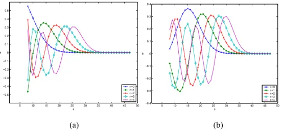
We first illustrate the influence of the parameter c on image reconstruction. A constant value is assigned to the parameter a, we arbitrarily set a = 8 for this example. Five cases have been tested in terms of the

constraints give by Eq. (15): (a) c = –8; (b) c = –4; (c) c = 0; (d) c = 4; (e) c = 8. Fig. 4 depicts the plots of dual Hahn polynomials with different values of c with N = 40. We can observe from Fig. 4 that the dual Hahn polynomials shift from left to right as c increases. We use a binary English character whose size is 40×40 pixels as original image to test the influence of the parameter c on the reconstruction results. The following mean square error ε is used to measure the performance of the reconstruction.

∑∑

− = − =

−

=

1 1 2 2

[

(

,

)

(

,

)]

1

b a s b a t

t

s

f

t

s

f

N

ε

(64) where f(s, t) and f( ts, )denote the original image and the reconstructed image, respectively. The reconstructed results and corresponding errors are shown in Table 3 and Fig. 5. It can be seen that the fifth choice (a = c = 8, b = 48) gives the best reconstructed results among all the test cases. We believe this is because the weighted dual Hahn polynomials, with this choice of parameters, are approximately situated at the middle of the region of definition (see Fig. 4 (e)), so that the emphasis of the moments will be at the center of the image.

In the following experiment, we will discuss the influence of parameter a on the reconstruction results.

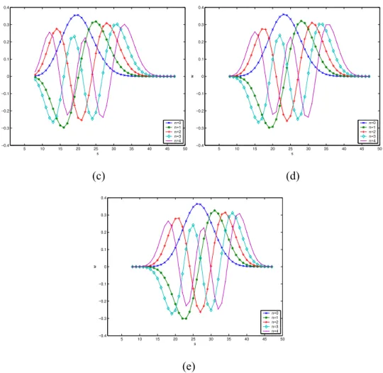
According to the above results and the constraints imposed on these parameters given in (15), we have systematically set a = c and b = a + N in all experiments. Fig. 6 shows several plots of dual Hahn

polynomials with increasing values of a where it can be observed that the dual Hahn polynomial moves from left to right. We then select a Chinese character whose size is 60 × 60 pixels as the original image. Three cases have been tested: (a) a = c = 0, and b = 60; (b) a = c = 7, and b = 67; (c) a = c = 18, and b = 78. Table 4 depicts the original image and the reconstructed patterns with a moment order going from 10 to 50. The plot of corresponding reconstruction errors is tabulated in Fig. 7. From Table 4 and Fig. 7, we can observe that the reconstructed images with a = c = 7, and b = 67, are better. For this parameter setting, the weighted dual Hahn polynomials are approximately situated at the middle of the region of definition (see Fig. 6(b)). It can be also seen that when the first choice is used, the reconstruction starts from top left corner, and with the third one, the reconstruction begins from bottom right corner. Therefore, the dual Hahn moments can be used to extract the feature of an image by adjusting the parameters. For dual Hahn moments, so far as a = c, the smaller of the value of a and c, the emphasis of the region-of-interest (ROI)

on the top left corner will be. Conversely, the ROI of the image shift to the bottom right corner when they take greater value. Note that the other selections (a = 6, a = 8, a = 9, and a = 10) have also been tested for this example, but the reconstruction results are very similar to those obtained with a = 7. From these results, we found if the parameters are set a = c and b = a + N, where N × N is the image size, a ≈ N/10 provides the best reconstruction.

4.2. Image reconstruction capability for binary image

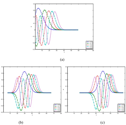
We use a noise-free binary Chinese character image to compare the performance of the proposed method with Legendre, Tchebichef and Krawtchouk moments. The image size is 60 × 60 pixels. Fig. 8 shows the reconstruction results. Note that the parameters are set to a = c = 7, and b = 67 for the proposed moments, and p1 = p2 = 0.5 is used in the Krawtchouk moments.

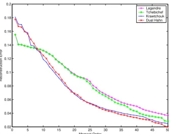
Fig. 9 displays the detailed plot of the mean square errors using four different orthogonal moments with maximum order up to 50. As it can be seen from Fig. 8 and Fig. 9, the reconstructed images using Krawtchouk and dual Hahn moments perform better than the other moments. When the moment order is high (M ≥ 25), the reconstruction error with dual Hahn moments is the smallest one.

4.3. Image reconstruction capability for gray-level image

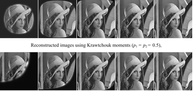
For this experiment, a gray-level standard image Lena of size 256 × 256 pixels is used to compare the performance the proposed dual Hahn moments with the other moments. Moments up to maximum order of 255 are computed from the original image, and the reconstruction results are illustrated in Fig. 10. A detailed comparison of the variation of reconstruction errors is shown in Fig. 11. It can be observed that these data confirm, both qualitatively and quantitatively, the good behavior highlighted above.

4.4. Robustness to different kind of noises

It is well known that the reconstruction quality can be severely affected by image noise. Generally speaking, moments of higher orders are more sensitive to image noise (Mukundan et al., 2001a). To further test the robustness of dual Hahn moments regarding to different kind of noises, we first add in this

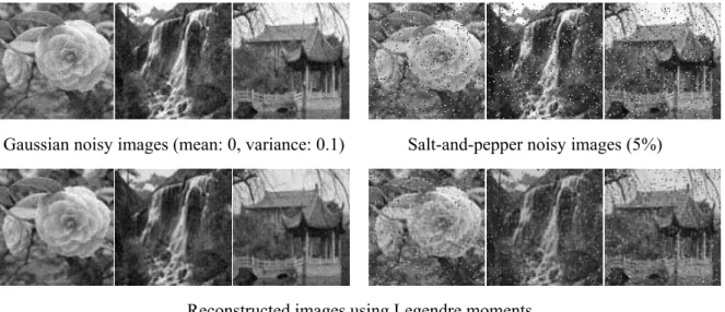
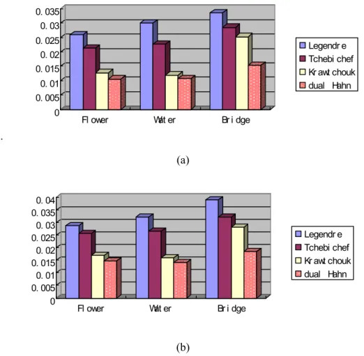
example a zero mean Gaussian noise with variance 0.1 to the three original gray-level images shown in the first row of Fig. 12. Fig. 12 depicts the reconstructed images using Legendre, Tchebichef, Krawtchouk, and dual Hahn moments. The reconstruction errors are shown in Fig. 13 (a) which again indicates the better performance of dual Hahn moments.

The effect of salt-and-pepper noise (5%) is also analyzed. The reconstructed images with the maximum order of moments up to 50 are shown in Fig. 12 and the mean square errors are reported in Fig. 13 (b). It can be seen that the dual Hahn moments is more robust to noise with respect to Legendre and Tchebichef moments, and that the Krawtchouk ones provide similar performances.

4.5. Invariant pattern recognition

This subsection provides the experimental study on the classification accuracy of dual Hahn moments in both noise-free and noisy conditions. In our classification task, we use the following feature vector.

] ~ , ~ , ~ , ~ , ~ , ~ [D₀₀ D₁₀ D₀₁ D₁₁ D₂₀ D₀₂ V = (65) where D~_nmare the dual Hahn moment invariants defined in Section 3.4. The objective of a classifier is to identify the class of the unknown input character. During classification, features of the unknown character are compared against the training information being assigned a particular class. The Euclidean distance measure is commonly used for classification purpose and is given by:

∑

= − = T j tj sj k t s V v v V d 1 2 ) ( _{) ( )} , ( (66)

where is the T-dimensional feature vector of unknown sample, and is the training vector of class

k. In this experiment, the classification accuracy s V (k) t V ηis defined as % 100 test in the used images of number total The images classified correctly of Number × = η (67)

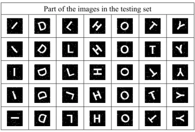
Fig. 14 shows a set of similar binary English characters used as the training set. The reason for choosing such a character set is that the elements in subset {I, L}, {D, O}, and {H, T, Y} can be easily misclassified due to the similarity. Seven testing sets are used, which are generated by adding different densities of salt-and-pepper noise add to the rotational version of each character. Each testing set is composed of 168

images, which are generated by rotating the training images every 45 degrees in the range [0, 360) and then by adding different densities of noises. Fig. 15 shows some of the testing images contaminated by 2% salt-and-pepper noise. The feature vector based on dual Hahn moment invariants are used to classify these images and its recognition accuracy is compared with that of Hu’s moment invariants (Hu, 1962). Table 5 shows the classification results using a full set of features. One can see from this table that 100% recognition results are obtained in noise-free case. Note that the recognition accuracy decreases when the noise is high. The second testing set is generated by rotating and scaling the training set with rotating angles, , , ,…, and scaling factors, S = 0.9, 1.0, 1,1; forming a testing set of 168 images. This is followed by the addition of salt-and-pepper noise similar to that of the first testing set. The classification results of the image with rotation and scaling transformation are depicted in Table 6. Table 6 shows that the better results are obtained with the dual Hahn invariant vector. Experimental results demonstrated that the dual Hahn moments perform better than the traditional Hu’s moments in terms of invariant pattern recognition accuracy in both noise-free and noisy conditions. Therefore, the dual Hahn moments could be useful as new image descriptors.

0 0 =

φ ₄₅0 ₉₀0 ₃₁₅0

5. Conclusion

The hypergeometric polynomials of continuous or discrete variable, whose canonical forms are the so-called classical orthogonal polynomial systems, play a crucial role in many scientific research fields. Recently, some sets of discrete orthogonal moment functions have been introduced in image processing. The discrete orthogonal moments based on discrete orthogonal polynomials, such as Tchebichef and Krawtchouk polynomials, have better image representation capability than the continuous orthogonal moments. These discrete orthogonal polynomials are the polynomial solutions of the difference equation on the uniform lattice.

In this paper, we have proposed the use of a new type of discrete orthogonal polynomials (so-called dual Hahn polynomials) on a non-uniform lattice to define the moments. It is noted that the reconstructed images still have uniform pixel lattices. The discrete Krawtchouk polynomials, discrete Tchebichef polynomials are special cases of dual Hahn polynomials. All of them are orthogonal in certain range. The

computational aspects and symmetry property of dual Hahn moments have been discussed in detail. In experimental studies, we have compared the dual Hahn moments with other orthogonal moments such as Legendre, Tchebichef and Krawtchouk moments in terms of the reconstruction capability with and without noise. The reconstruction results and detailed error analysis have shown that the dual Hahn moments perform better than other moment’s methods. Pattern classification experiments also demonstrated that the dual Hahn moments perform better than the Hu’s moment invariants in terms of invariant pattern recognition accuracy in both noise-free and noisy conditions. To conclude, the discrete dual Hahn moments are potentially useful as feature descriptors for image analysis, and the method described in this paper can be easily extended to the construction of moment functions from other discrete orthogonal polynomials on the non-uniform lattice.

Acknowledgement: This work was supported by National Basic Research Program of China under grant No.2003CB716102, the National Natural Science Foundation of China under grant No. 60272045, and Program for New Century Excellent Talents in University under grant No. NCET-04-0477. We thank the anonymous referees for their helpful comments and suggestions.

Appendix A

In this appendix, we give a detailed derivation of the recurrence relation with respect to n

According to Nikiforov and Uvarov (1988), we can construct the recursive relation for dual Hahn orthogonal polynomials as follows

) ( ) ( ) ( ) (x y ₁ x y x y ₁ x xy_n =α_{n n+} +β_{n n} +γ_{n n−} (A1) with α_n = n+1 (A2) 2 2 ) 1 2 )( 1 (b a c n n bc ac ab n= − + + − − − + − β (A3) ) )( )( (a c n b a n b c n n = + + − − − − γ (A4)

Using equations (A1)-(A4), we have

) ( ) ( ) (x Ay ₁ x By ₂ x y_n = _n− + _n− (A5) with ] ) 1 ( 2 ) 1 2 )( 1 ( ) 1 ( [ 1 ] ) 1 ( 2 ) 1 2 )( 1 ( [ 1 2 2 − + − − − − − − + − + = − + − − − − − − + − = n n c a b bc ac ab s s n n n c a b bc ac ab x n A (A6) ) 1 )( 1 )( 1 ( 1 _{+ + − − − + − − +} − = a c n b a n b c n n B (A7)

For dual Hahn orthogonal polynomial, in (A5) is defined as . From equations (21) and (A5), we can obtain the weighted dual Hahn polynomials in recursive form as

) (x y_{n w}(c)(_s,_a,_b) n ) , , ( ˆ ) , , ( ˆ ) , , ( ˆ ( ) 2 2 ) ( 1 1 ) ( _{w s a b} d d B b a s w d d A b a s w c n n n c n n n c n = − − + − − (A8) where ) )( )( ( 2 2 1 n c b n a b n c a n d d n n − − − − + + = − _(A9) ) )( 1 )( )( 1 )( 1 )( ( ) 1 ( 2 2 2 n c b n c b n a b n a b n c a n c a n n d d n n − − + − − − − + − − − + + + + − = − _(A10)

The initial value of ( )( , , )and (see equations (29) and (30)) can be obtained from (8) as 0 s a b wc ( )_{( , , )} 1 s a b wc )] ( [ ) ( ) ( ( ) _s s B s P n _n n n n = _ρ ∇ ρ (A11)

where _P(_s) _w(c)(_s,_a,_b), and is defined as follows(Nikiforov and Uvarov, 1988)

n n ≡ Bn ! / ) 1 ( n B n n = − (A12) thus 1 ) ( ) ( ) , , ( 0 ₀ ) ( 0 = ⋅ s = s B b a s wc _ρ ρ (A13) ) 2 1 ( ) 2 1 ( ) 1 ( ) ( ) ( 1 ) ( ) ( ) ( ) , , ( 1 1 1 1 1 ) ( 1 − − + − − ⋅ − = ⋅ ∇ ∇ ⋅ = s x s x s s s s s x s B b a s wc ρ ρ ρ ρ ρ (A14)

Finally, the original values ˆ( )( , , )and can be obtained from (21). 0 s a b

wc _ˆ( )_{( , , )} 1 s a b

wc

Appendix B

In this appendix we derive the recurrence relation (38) of discrete dual Hahn polynomials. By using equation (5) and x(s) = s (s + 1), we can be rewritten the first term of (5) as

⎥ ⎦ ⎤ ⎢ ⎣ ⎡ ₋ − − + − + + = − − ⋅ + = ∇ ∇ ⋅ + = ∇ ∇ − s s y s y s s y s y s s s s y s y s s s x s y s s s x s y s x s 2 ) 1 ( ) ( ) 1 ( 2 ) ( ) 1 ( 1 2 ) ( ] 2 ) 1 ( ) ( [ 1 2 ) ( ] ) ( ) ( [ 1 2 ) ( ] ) ( ) ( [ ) 2 1 ( ) ( σ σ σ σ Δ Δ Δ Δ (B1)

Similarly, the second term of (5) can also be rewritten as

) 1 ( 2 ) ( ) 1 ( ) ( ] ) ( ) ( )[ ( + − + = s s y s y s s x s y s τ τ Δ Δ (B2)

From (5), (B1), and (B2), we have

0 ) 2 ( ) 1 ( ) 1 ( ))] 1 ( 2 ) 1 ( ) 1 ( ) 1 ( )( 2 1 [( ) ( )] 1 ( ) 1 2 ( ) 1 ( )[ 1 ( = − ⋅ − ⋅ + − − ⋅ + − ⋅ − + − − + − ⋅ − + − − s y s s s y s s s s s s s y s s s s σ λ τ σ τ σ (B3)

where y(s) denotes the dual Hahn polynomials_w(c)(_s,_a,_b).

n

Equation (38) can thus be derived from (B3) and (21). To obtain the initial value of_w(c)(_s,_a,_b), we

n

use the Rodrigues formula (8). )] 0 ( [ ) 0 ( ) 0 ( n (_nn) _n n B P ρ ρ ∇ = (B4)

where P_n(0)≡w_n(c)(0,a,b). Using (33) and (B4), we have

n n n n n c n _{n n} a c b n B b a w ( 1) ( 1) ( ) ) ! ( 1 ! ) 0 ( ) 0 ( ) , , 0 ( ₂ ) ( _{= ⋅}ρ _{=− + + −} ρ (B5) Similarly, P(1) w(c)(1,a,b) n n ≡ ) , , 0 ( 2 ) 1 ( ) 0 ( ) 1 ( ) 1 ( ) 0 ( ) 1 )( 2 ( 2 ) , , 0 ( ) 2 ( ) 1 )( 2 ( 2 ) 0 ( ) 1 ( ) 1 ( ) 0 ( )! 2 ( ) 1 ( )! 2 )( 0 ( ) 1 ( 2 ) 0 ( ! ! ) 1 ( ) 0 ( ) 0 ( ) 0 ( )! 2 ( ) 1 ( ) 1 ( )! 2 ( 2 ) 1 ( ) , , 1 ( ) ( ) ( ) ( b a w n n n n b a w n n n n n n n n n n B n n n n B b a w c n n n c n n n n n n n n n n c n ⎥ ⎦ ⎤ ⎢ ⎣ ⎡ + − ⋅ + + = ⎥ ⎦ ⎤ ⎢ ⎣ ⎡ + − + + ⋅ ⋅ = ⎥ ⎦ ⎤ ⎢ ⎣ ⎡ + + − + ⋅ ⋅ ⋅ = ⎥ ⎦ ⎤ ⎢ ⎣ ⎡ ⋅ + + − ⋅ + ⋅ = ρ ρ ρ ρ ρ ρ ρ ρ ρ ρ ρ ρ ρ ρ ρ ρ ρ (B6)

Using equations (21), (B5) and (B6), we can obtain the weighted initial values of dual Hahn polynomials shown in (39) and (40).

References

Álvarez-Nodarse, R., Arvesú, J., Yáñez, R.J., 2001a. On the connection and linearization problem for discrete hypergeometric q-polynomials. J. of Math. Anal. Appl. 257(1), 52-78.

Álvarez-Nodarse, R., Costas-Santos, R.S., 2001b. Factorization method for difference equations of hypergeometric type on nonuniform lattice. J. Phys. A: Math. Gen. 34, 5551-5569.

Álvarez-Nodarse, R., Smirnov, Y.F., 1996. The Dual Hahn q-polynomials in the lattice x(s)=[s]q[s+1]q

and the q-algebras SUq(2) and SUq(1,1). J. Phys. A: Math. Gen. 29, 1435-1451.

Arvesú, J., Coussement, J., Assche, W.V., 2003. Some discrete multiple orthogonal polynomials. J. Comput. Appl. Math. 153(1), 19-45.

Chong, C.W., Raveendran, P., Mukundan, R., 2003. A comparative analysis of algorithms for fast computation of Zernike moments. Pattern Recognition. 36(3), 731-742.

Foupouagnigni, M., Ronveaux, A., 2003. Difference equations for the co-recursive rth associated orthogonal polynomials of the Dq-Laguerre-Hahn class. J. Comput. Appl. Math. 153, 213-223.

Hu, M.K., 1962. Visual pattern recognition by moment invariants. IRE Trans. Inform. Theory 8, 179-187. Kiryati, N., Bruckstein, A.M., Mizrahi, H., 2000. Comments on: Robust line fitting in a noisy image by

the method of moments. IEEE Trans. Pattern Anal. Machine Intell.12(11), 1340-1341.

Koekoek, R., Swarttouw, R., 1998. The Askey-scheme of hypergeometric orthogonal polynomials and its

q-analogue, Report 98-17, Fac. Techn. Math. Informatics, Delft University of Technology. Delft.

Koepf, W., Schmersau, D., 2001. On a structure formula for classical q-orthogonal polynomials. J. Comput. Appl. Math. 136, 99-107.

Kupershmidt, B.A., 2003. Q-analogs of classical 6-periodicity: from Euler to Chebyshev. J. Nonlinear Math. Phys. 10(3), 318-339.

Mandal, M.K., Aboulnasr, T., Panchanathan, S., 1996. Image indexing using moments and wavelets. IEEE Trans. Consumer Electron. 42(3), 557-565.

Mukundan, R., Ong, S.H., Lee, P.A., 2001a. Discrete vs. continuous orthogonal moments for image analysis. Internationa. Conf. on Imaging Science, Systems and Technology-CISST’01, Las Vegas, 23-29.

Mukundan, R., Ong, S.H., Lee, P.A., 2001b. Image analysis by Tchebichef moments. IEEE Trans. Image Process. 10(9), 1357-1364.

Mukundan, R., 2004. Some computational aspects of discrete orthonormal moments. IEEE Trans. Image Process. 13(8), 1055-1059.

Nikiforov, A.F., Uvarov, V.B., 1988. Special functions of mathematical physics. Birkhauser, Basel Boston. Qing, C., Emil, P., Xiaoli, Y., 2004. A comparative study of Fourier descriptors and Hu's seven moment

invariants for image recognition. Canadian Conference on Electrical and Computer Engineering 1(2-5), 103-106.

Ronveaux, A., Zarzo, A., Area, I., Godoy, E., 2000. Classical orthogonal polynomials: dependence of parameters. J. Comput. Appl. Math. 121(1-2), 95-112.

Shu, H. Z., Luo, L. M., Yu, W. X., Fu, Y., 2000. A new fast method for computing Legendre moments. Pattern Recognition 33, 341-348.

Talenti, G., 1987. Recovering a function from a finite number of moments. Inverse Problem. 3, 501-517. Teague, M.R., 1980. Image analysis via the general theory of moments. J. Opt. Soc. Amer. 70(8),

920-930.

Temme, N.M., López, J.L., 2000. The Askey scheme for hypergeometric orthogonal polynomials viewed from asymptotic analysis. Technology Report, MAS-R0005.

Vega, H.J., 1989. Yang-Baxter algebras, integral theories and quantum groups. Int. J. Mod. Phys. 2371-2463.

Yap, P.T., Paramesran, R., Ong, S.H., 2003. Image Analysis by Krawtchouk Moments. IEEE Trans Image Process. 12(11), 1367-1377.

Yin, J.H., Pierro, A.R.D., Wei, M., 2002. Analysis for the reconstruction of a noisy signal based on orthogonal moments. Appl. Math. Computat. 132(2), 249-263.

Zhu, H.Q., Shu, H.Z., Liang J., Luo, L.M., Coatrieux, J.L., 2007. Image analysis by discrete orthogonal Racah moments. Signal Process. 87, 687-708.

Table 1

Some important discrete orthogonal polynomials on the non-uniform lattice (p, q, a, b, c, γ, μ, α, β, and ω

are parameters attached to the respective polynomials, n denoting the order)

Name Notation Lattice smin smax ρ(s)

dual Hahn w(_nc)(s,a,b) x(s) = s(s + 1) a b ) 1 ( ) 1 ( ) ( ) 1 ( ) 1 ( ) 1 ( + − Γ + + Γ − Γ + − Γ + + Γ + + Γ c s s b s b a s s c s a Racah u_n(α,β)(s,a,b) x(s) = s(s + 1) a b ) 1 ( ) ( ) 1 ( ) 1 ( ) 1 ( ) ( ) 1 ( ) 1 ( + + Γ − Γ + − Γ + + − Γ + + + Γ − + Γ + + − Γ + + Γ s b s b a s s a s b s b a s s a β α α β q-Krawtchouk k_n(p)(s,N,q) x(s) = q2s 0 N ) 1 ( ) 1 ( ]! [ ) 1 ( s N s N q q q s s s − + Γ Γ − ＋ μ _{, μ=p/(1−p)} q-Meixner m_n(r,μ)(s,q) x(s) = q2s 0 ∞ ) 1 ( ) ( ) ( + Γ Γ + Γ s r s r q q q s μ q-Hahn wn(c)(s,a,b)q x(s)=[s]q[s+1]q a b _{[ ] ![ ]![ ] ![ 1]!} ! ] [ ! ] [ ) 1 ( q q q q q q s s s b b s c s a s c s a s q − − + − − + + + − Table 2

Comparison of dual Hahn moments and Racah moments.

Moment Polynomials Symmetry Number of

Parameters

Reconstruction Capability

Compression Capability

dual Hahn Relatively Simple: ₂F₃

Orthogonal About n Three:(a, b, c) Very Good Good

Racah More Complex: ₃F₄ Orthogonal About n + a and s only if a = α = β Four:(a, b, α, β)

Good Very Good

Table 3

Image reconstruction of the letter “F” of size (40×40) without noises, a = 8, b = 48 Original Image (40×40) Reconstructed Image Iterative Number c =−8 c =− 4 c = 0 c = 4 c = 8 1 5 15 39 Table 4

Image reconstruction of the Chinese character of size 60 × 60 without noises Original Image (60 × 60) Reconstructed Image Iterative number a = c = 0, b = 60 a = c = 7, b = 67 a = c = 18, b = 78 10 20 30 50

Table 5

Classification results of the image with rotation transformation

Salt-and-pepper Noise Noise-free 1% 2% 3% 4% Hu 100% 96.62% 87.047% 75.76% 70.83% Dual Hahn 100% 98.22% 92.88% 81.57% 78.67% Table 6

Classification results of the image with Rotation and Scaling transformation. Scale: 0.9, 1, 1.1

Rotation: 00, 450, 900,……. Salt-and-pepper Noise Noise-free 1% 2% 3% 4% Hu 98.70% 89.02% 78.01% 72.16% 65.81% Dual Hahn 98.75% 92.53% 82.48% 79.31% 75.74% 5 10 15 20 25 30 35 40 −0.3 −0.2 −0.1 0 0.1 0.2 0.3 0.4 s w n=0 n=1 n=2 n=3 n=4

Fig.1. Plot of scaled of dual Hahn polynomials

_w

_w

ˆ

(c)

(

_s

,

_a

,

_b

)

for N = 40 with a = c = 0,

n

=

and b = 40.