Numer. Math. (2012) 120:307–343 DOI 10.1007/s00211-011-0408-x
Numerische Mathematik
Reconstructing initial data using observers:
error analysis of the semi-discrete and fully discrete approximations
Ghislain Haine · Karim Ramdani
Received: 24 August 2010 / Revised: 10 May 2011 / Published online: 11 September 2011
© Springer-Verlag 2011
Abstract A new iterative algorithm for solving initial data inverse problems from partial observations has been recently proposed in Ramdani et al. (Automatica 46(10), 1616–1625,2010). Based on the concept of observers (also called Luenberger observ- ers), this algorithm covers a large class of abstract evolution PDE’s. In this paper, we are concerned with the convergence analysis of this algorithm. More precisely, we provide a complete numerical analysis for semi-discrete (in space) and fully discrete approximations derived using finite elements in space and an implicit Euler method in time. The analysis is carried out for abstract Schrödinger and wave conservative systems with bounded observation (locally distributed).
Mathematics Subject Classification (2000) Primary 35Q93; Secondary 35L05· 35J10·65M22
1 Introduction
The goal of this paper is to present a convergence analysis for the iterative algorithm recently proposed in Ramdani et al. [24] for solving initial state inverse problems from measurements over a time interval. This algorithm is based on the use back and forth in time of observers (sometimes called Luenberger observers or Kalman observers;
see for instance Curtain and Zwart [6]). Inspired by the works of Mathias Fink on time
G. Haine
Université Henri Poincaré (Institut Élie Cartan), B.P. 70239, 54506 Vandoeuvre, France, e-mail: [email protected]
K. Ramdani (
B
)INRIA Nancy Grand-Est (CORIDA), 615 rue du Jardin Botanique, 54600 Villers, France e-mail: [email protected]
reversal [9,10], Phung and Zhang [22] used this algorithm in the particular case of the Kirchhoff plate equation with distributed observation, while Ito et al. [15] considered more general evolution PDE’s with locally distributed observation. Let us mention also Auroux and Blum [1] who implemented a similar algorithm in the context of data assimilation. More generally, during the last decade, observers have been designed for linear and nonlinear infinite-dimensional systems in many works, among which we can mention for instance Deguenon et al. [8], Guo and Guo [13], Guo and Shao [14] in the context of wave-type systems, Lasiecka and Triggiani [19], Smyshlyaev and Krstic [26] for parabolic systems and Krstic et al. [17] for the non linear viscous Burgers equation.
Let us first briefly describe the principle of the reconstruction method proposed in [24] in the simplified context of skew-adjoint generators and bounded observa- tion operator. We will always work under these assumptions throughout the paper.
Given two Hilbert spaces X and Y (called state and output spaces respectively), let A : D(A) → X be skew-adjoint operator generating a C0-group Tof isometries on X and let C ∈ L(X,Y)be a bounded observation operator. Consider the infinite dimensional linear system given by
z(t˙ )= Az(t), ∀t0,
y(t)=C z(t), ∀t∈ [0, τ]. (1.1) where z is the state and y the output function (throughout the paper, the dot symbol is used to denote the time derivative). Such systems are often used as models of vibrating systems (e.g., the wave equation, the beam equation,…), electromagnetic phenomena (Maxwell’s equations) or in quantum mechanics (Schrödinger’s equation).
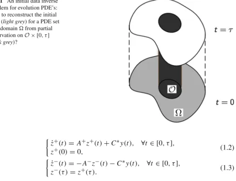
The inverse problem considered here is to reconstruct the initial state z0=z(0)of system (1.1) knowing (the observation) y(t)on the time interval[0, τ](see Fig.1).
Such inverse problems arise in many applications, like thermoacoustic tomography Kuchment and Kunyansky [18] or data assimilation Puel [23]. To solve this inverse problem, we assume here that it is well-posed, i.e. that(A,C)is exactly observable in timeτ >0. In other words, we assume that there exists kτ >0 such that
τ 0
y(t)2dt ≥kτ2z02, ∀z0∈D(A).
For instance, in the case of the wave equation on a bounded domain, this inequality holds provided we observe the state onO×(0, τ)whereO ⊂andτ are chosen such that the geometric optics condition of Bardos et al. [2] holds. For similar results related to other equations, see for instance Burq [3], Burq and Lebeau [4] and Jaffard [16] and the monograph of Lions [20].
Following Liu [21, Theorem 2.3.], we know that A+ = A−C∗C (respectively A−= −A−C∗C) generate an exponentially stable C0-semigroupT+(respectively T−) on X . Then, we introduce the following initial and final Cauchy problems, called respectively forward and backward observers of (1.1)
Fig. 1 An initial data inverse problem for evolution PDE’s:
How to reconstruct the initial state (light grey) for a PDE set on a domainfrom partial observation onO× [0, τ]
(dark grey)?
z˙+(t)= A+z+(t)+C∗y(t), ∀t ∈ [0, τ],
z+(0)=0, (1.2)
z˙−(t)= −A−z−(t)−C∗y(t), ∀t ∈ [0, τ],
z−(τ)=z+(τ). (1.3)
Note that the states z+ and z− of the forward and backward observers are com- pletely determined by the knowledge of the output y. If we setLτ =T−τT+τ, then by [24, Proposition 3.7], we haveη:= LτL(X) <1 and by [24, Proposition 3.3], the following remarkable relation holds true
z0=(I −Lτ)−1z−(0). (1.4)
In particular, one can invert the operator(I−Lτ)using a Neumann series and get the following expression for the initial state
z0=∞
n=0
Lnτz−(0). (1.5)
Thus, at least theoretically, the reconstruction of the initial state is given by the above formula. Note that the computation of the first term in the above sum requires to solve the two non-homogeneous systems (1.2) and (1.3), while the terms for n≥1 involve the resolution of the two homogeneous systems associated with (1.2) and (1.3) (i.e. for y ≡0). In practice, the reconstruction procedure requires the discretization of these two systems and the truncation of the infinite sum in (1.5) to keep only a finite number of back and forth iterations. For instance, if we consider a space semi-discretization corresponding to a mesh size h (typically a finite element approximation), one can only compute
z0,h=
Nh
n=0
Lnh,τz−h(0), (1.6)
where
– Lh,τ =T−h,τT+h,τ, whereT±h,τ ∈L(X)are suitable space discretizations ofT±τ, – z−h(0)∈ Xhis an approximation of z−(0)in a suitable finite dimensional subspace
Xhof X ,
– Nhis a suitable truncation parameter.
Similarly, if a full discretization described by a mesh size h and a time stept is considered, one can compute
z0,h,t =
Nh,t
n=0
Lnh,t,K z−h0
. (1.7)
where
– Lh,t,K =T−h,t,KT+h,t,K, whereT±h,t,Kare suitable space and time discretiza- tions ofT±τ,
–
z−h0
∈ Xhis an approximation of z−(0), – Nh,t is a suitable truncation parameter.
For the sake of clarity, the precise definition of the spaces and discretizations used will be given later in the paper.
Our objective in this work is to present a convergence analysis of z0,hand z0,h,t
towards z0. A particular attention will be devoted to the optimal choice of the trun- cation parameters Nhand Nh,tfor given discretization parameters (mesh size h and time stept ). Let us emphasize that our error estimates (see (2.8), (2.27), (3.15) and (3.25)) provide in particular an upper bound for the maximum admissible noise under which convergence of the algorithm is guaranteed. As usually in approximation error theory of PDE’s, some regularity assumptions are needed to obtain our error esti- mates. Namely, our result allows us to reconstruct only initial data contained in some subspace of X (namelyD
A2 ).
Let us emphasize that similar error estimates have been recently obtained by Cîndea et al. [5] in the context of control problems. Using Russel’s “stabilizability implies controllability” principle, the authors derived a new approximation method of exact controls for second order wave type systems with bounded input operator. The con- vergence analysis is carried out in the case of a Galerkin type semi-discretization.
Let us now make some comments on the type of observation for which we have been able to prove convergence results. First of all, we assume throughout the paper that C∈L(X,Y)is a bounded observation operator (locally distributed observation).
This assumption is crucially used many times in the proofs and it seems difficult to extend our result to the case of unbounded observation. However, the reconstruction algorithm seems to be still efficient in this case, as it can be seen from the numerical results given in [24].
In addition to the boundedness of C, we assume that C∗C ∈ L D
A2 L(D(A)). The fact that C∗C ∈ L(D(A)) ensures that the contraction property∩ forT+andT−is still satisfied when restricted toD(A)andD
A2
(see Lemma1 of the Appendix). Let us point out that this is proved for the damped wave equation in Cîndea et al. [5, Proposition 2.5]. Moreover, we also haveLτD(A) < 1 and LτD(A2) < 1 (by application of [27, Proposition 2.10.4]). The second technical assumption C∗C ∈ L
D A2
appears naturally in our analysis, but not in the one carried out in Cîndea et al. [5]. Indeed, this assumption is used to bound a term which does not appear in the context of control problems they considered. Finally, let us point out that these assumptions are in particular satisfied when the locally distributed observation is obtained via a smooth cut-off function.
Remark 1 Using an implicit Euler method preserves the dissipative properties of the high frequency part of the solution (see (2.30) and (3.30)). This is the main reason for which we did not use an explicit or midpoint Euler scheme, but we do not know if this restriction is only technical or not.
The paper is organized as follows: in Sect.2we provide a convergence analysis of the algorithm for an abstract Schrödinger type system, by considering successively the semi-discretization (Sect.2.1) and the full discretization (Sect.2.2). In Sect.3, similar results are given for an abstract wave system. Once again, we tackle successively the semi-discretization (Sect.3.1) and the full discretization (Sect.3.2). However, since the proofs are very similar to those of the Schrödinger case, they will not be given with full details. Finally, the Appendix is devoted to the proof of two technical lemmas which are used several times throughout the paper.
Throughout the paper, we denote by M a constant independent ofτ, of the initial state z0and of the discretization parameters h andt , but which may differ from line to line in the computations.
2 Schrödinger equation
Let X be a Hilbert space endowed with the inner product·,·. Let A0:D(A0)→X be a strictly positive self-adjoint operator and C ∈ L(X,Y)a bounded observation operator, where Y is an other Hilbert space. The norm in D(Aα0)will be denoted by · α. We assume that there exists some τ > 0 such that(i A0,C) is exactly observable in time τ. Thus by Liu [21, Theorem 2.3.], A+ = i A0−C∗C (resp.
A− = −i A0−C∗C) is the generator of an exponentially stable C0-semigroupT+ (resp.T−). We want to reconstruct the initial value z0of the following system
z˙(t)=i A0z(t), ∀t 0,
y(t)=C z(t), ∀t∈ [0, τ]. (2.1) Throughout this section we always assume that z0∈D
A20
. Thus by applying The- orem 4.1.6 of Tucsnak and Weiss [27], we have
z∈C
[0, τ],D A20
∩C1([0, τ],D(A0)) .
The forward and backward observers (1.2) and (1.3) read then as follows ˙z+(t)=i A0z+(t)−C∗C z+(t)+C∗y(t), ∀t ∈ [0, τ],
z+(0)=0, (2.2)
˙z−(t)=i A0z−(t)+C∗C z−(t)−C∗y(t), ∀t ∈ [0, τ],
z−(τ)=z+(τ). (2.3)
Clearly, the above systems can be rewritten in the general form of an initial value Cauchy problem (simply by using a time reversal for the second system)
q˙(t)= ±i A0q(t)−C∗Cq(t)+F(t), ∀t ∈ [0, τ],
q(0)=q0, (2.4)
where we have set
– for the forward observer (2.2) : F(t)=C∗y(t)=C∗C z(t)and q0=0,
– for the backward observer (2.3) : F(t) = C∗y(τ −t) = C∗C z(τ −t) and q0=z+(τ)∈D
A20 . 2.1 Space semi-discretization 2.1.1 Statement of the main result
We use a Galerkin method to approximate system (2.4). More precisely, consider a family(Xh)h>0of finite-dimensional subspaces ofD A
1 2
0
endowed with the norm in X . We denoteπhthe orthogonal projection fromD A
1 2
0
onto Xh. We assume that there exist M>0, θ >0 and h∗>0 such that we have for all h∈(0,h∗)
πhϕ−ϕ ≤M hθϕ1
2 , ∀ϕ∈D A
1 2
0
. (2.5)
Given q0∈D A20
, the variational formulation of (2.4) reads for all t∈ [0, τ]and all ϕ∈D A
1 2
0
as follows
˙q(t), ϕ = ±iq(t), ϕ1
2 − C∗Cq(t), ϕ + F(t), ϕ,
q(0)=q0. (2.6)
Suppose that q0,h∈Xhand Fhare given approximations of q0and F respectively in the spaces X and L1([0, τ],X). For all t∈ [0, τ], we define qh(t)∈ Xhas the unique solution of the variational problem
˙qh(t), ϕh = ±iqh(t), ϕh1
2 − C∗Cqh(t), ϕh + Fh(t), ϕh,
qh(0)=q0,h. (2.7)
for allϕh ∈Xh.
The above approximation procedure leads in particular to the definition of the semi- discretized versionsT±h of the semigroupsT±that we will use. Indeed, we simply set
T+t q0T+h,tq0=qh(t) T−t q0T−h,tq0=qh(τ−t)
where qhis the solution of Eq. (2.7) with the corresponding sign and for Fh=0 and q0,h=πhq0. The approximation ofLτ =T−τT+τ follows immediately by setting
Lh,τ =T−h,τT+h,τ.
Assume that yhis an approximation of the output y in L1([0, τ],Y)and let zh+and z−h denote the Galerkin approximations of the solutions of systems (2.2) and (2.3), satisfying for all t∈ [0, τ]and allϕh ∈Xh
˙ z+h(t), ϕh
=i
z+h(t), ϕh
1
2 −
C∗C z+h(t), ϕh
+ C∗yh(t), ϕh, zh+(0)=0.
˙ z−h(t), ϕh
=i
z−h(t), ϕh
1
2 +
C∗C z−h(t), ϕh
− C∗yh(t), ϕh, zh−(τ)=z+h(τ).
Thus, our main result in this subsection reads as follows.
Theorem 1 Let A0 : D(A0) → X be a strictly positive self-adjoint operator and C ∈ L(X,Y) such that C∗C ∈ L
D A20
∩L(D(A0)). Assume that the pair (i A0,C) is exactly observable in timeτ > 0 and set η := LτL(X) < 1. Let z0∈D
A20
be the initial value of (2.1) and z0,hbe defined by (1.6).
Then there exist M>0 and h∗>0 such that for all h∈(0,h∗)
z0−z0,h ≤M
⎡
⎣ ηNh+1
1−η +hθτNh2
z02+Nh
τ 0
C∗(y(s)−yh(s))ds
⎤
⎦.
A particular choice of Nh leads to an explicit error estimate (with respect to h) as shown in the next Corollary (the proof is left to the reader because of its simplicity) Corollary 1 Under the assumptions of Theorem1, we set
Nh=θln h lnη.
Then, there exist Mτ >0 and h∗>0 such that for all h∈(0,h∗) z0−z0,h ≤Mτ
⎛
⎝hθln2hz02+ |ln h|
τ 0
C∗(y(s)−yh(s))ds
⎞
⎠. (2.8)
Remark 2 In fact, Theorem1still holds true for z0∈D A
3 2
0
(with the same proofs and slightly adapting the spaces). Nevertheless, we have not been able to carry out this analysis for the fully discrete approximation in this case. This is why we restricted our analysis to the case of an initial data z0∈D
A20 . 2.1.2 Proof of Theorem1
Before proving Theorem1, we first need to prove some auxiliary results. The next Proposition, which constitutes one of the main ingredients of the proof, provides the error estimate for the approximation in space of the initial value problem (2.6) by using the Galerkin scheme (2.7).
Proposition 1 Given q0 ∈ D A20
and q0,h ∈ Xh, let q and qh be the solutions of (2.6) and (2.7) respectively. Assume that C∗C ∈L(D(A0)). Then, there exist M >0 and h∗>0 such that for all t ∈ [0, τ]and all h∈(0,h∗)
πhq(t)−qh(t) ≤ πhq0−q0,h +M hθ
t
q02+ F1,∞
+t2F2,∞
+ t 0
F(s)−Fh(s)ds,
whereFα,∞=supt∈[0,τ]F(t)α.
Proof First, we substract (2.7) from (2.6) and obtain (we omit the time dependence for the sake of clarity) for allϕh∈ Xh
˙q− ˙qh, ϕh = ±iq−qh, ϕh1
2 −
C∗C(q−qh), ϕh
+ F−Fh, ϕh.
Noting thatπhq−q, ϕh1
2 =0 for allϕh ∈ Xhand thatπhq makes sense by the˙ regularity of q (see (4.1)), we obtain from the above equality that for allϕh∈Xh
πhq˙− ˙qh, ϕh = πhq˙− ˙q, ϕh ±iπhq−qh, ϕh1
2
−
C∗C(q−qh) , ϕh
+ F−Fh, ϕh. (2.9)
On the other hand, setting
Eh=1
2πhq−qh2, we have
E˙h =Reπhq˙− ˙qh, πhq−qh.
Applying (2.9) withϕh =πhq−qhand substituting the result in the above relation, we obtain by using Cauchy-Schwarz inequality and the boundedness of C that there exists M >0 such that
E˙h≤(πhq˙− ˙q +Mπhq−q + F−Fh)π hq−qh
=√ 2Eh
.
Since √E˙h 2Eh = d
dt
√2Eh, the integration of the above inequality from 0 to t yields
πhq(t)−qh(t) ≤ πhq0−q0,h+ t 0
(πhq˙(s)− ˙q(s)+Mπhq(s)−q(s))ds
+ t 0
F(s)−Fh(s)ds. (2.10)
Thus, it remains to boundπhq(t)˙ − ˙q(t)andπhq(t)−q(t)for all t ∈ [0, τ].
Using (2.5) and the classical continuous embedding fromD(Aα)toD(Aβ)forα > β, we get that
πhq˙(t)− ˙q(t) ≤M hθ ˙q(t)1
2 ≤M hθ ˙q(t)1, πhq(t)−q(t) ≤M hθq(t)1
2 ≤M hθq(t)2, ∀t∈ [0, τ], h∈(0,h∗).
Using relations (4.2) and (4.3) proved in Lemma2 of the Appendix, we get for all t ∈ [0, τ]and all h∈(0,h∗)
πhq˙(t)− ˙q(t) + πhq(t)−q(t) ≤M hθ
q02+tF2,∞+ F1,∞
. Substituting the above inequality in (2.10), we get the result.
Using the last result, we derive an error approximation for the semigroupsT±and for the operatorLt =T−t T+t .
Proposition 2 Under the assumptions of Proposition1, the following assertions hold true
1. There exist M>0 and h∗>0 such that for all t∈(0, τ)and all h∈(0,h∗) πhT+t q0−T+h,tq0≤ Mt hθq02. (2.11)
πhT−t q0−T−h,tq0≤M(τ−t)hθq02. (2.12) 2. There exist M >0 and h∗ > 0 such that for all n ∈ N, all t ∈ [0, τ]and all
h∈(0,h∗), we have
Lntq0−Lnh,tq0 ≤M(1+nτ)hθq02. (2.13)
Proof
1. It suffices to take F=Fh=0 and q0,h=πhq0in Proposition1.
2. We first note that
Lntq0−Lnh,tq0 ≤ Lntq0−πhLntq0 + πhLntq0−Lnh,tq0. (2.14) Using (2.5) and the fact thatLtL(D(A)) ≤1 proved in Lemma1of the Appendix, the first term in the above relation can be estimated as follows
Lntq0−πhLntq0 ≤M hθq02, ∀h∈(0,h∗). (2.15) For the second term in (2.14), we prove by induction that for all n ∈N
πhLntq0−Lnh,tq0 ≤Mnτhθq02, ∀h∈(0,h∗). (2.16) By definition, we have
πhLtq0−Lh,tq0 = πhT−t T+t q0−T−h,tT+h,tq0,
≤ πhT−t T+t q0−T−h,tT+t q0 + T−h,t(T+t q0−T+h,tq0).
By Lemma1of the Appendix and Eq. (2.12), we get
πhT−t T+t q0−T−h,tT+t q0 ≤M(τ−t)hθq02, ∀h ∈(0,h∗).
ObviouslyT−hL(X)is uniformly bounded with respect to h (this follows for example from (2.12)), and thus by (2.5) and Eq. (2.11), we have
T−h,t(T+t q0−T+h,tq0) ≤ T+t q0−πhT+t q0 + πhT+t q0−T+h,tq0
≤Mt hθq02, ∀h∈(0,h∗).
Consequently
πhLtq0−Lh,tq0 ≤Mτhθq02, ∀h ∈(0,h∗), (2.17) which shows that (2.16) holds for n=1. Suppose now that for a given n≥2, there holds
πhLnt−1q0−Lnh−,t1q0 ≤M(n−1)τhθq02. (2.18) We write
πhLntq0−Lnh,tq0 ≤ πhLtLnt−1q0−Lh,tLnt−1q0 + Lh,t(Lnt−1q0−Lnh−,t1q0).
Thanks to Lemma1of the Appendix and to the uniform boundedness ofLh,tL(X)
with respect to h (which follows from the uniform boundedness ofT±h,t) and using (2.17) and (2.18), we obtain
πhLntq0−Lnh,tq0 ≤M(τ+(n−1)τ)hθq02,
which is exactly (2.16). Substituting (2.15) and (2.16) in (2.14), we obtain the result.
We are now able to prove Theorem1.
Proof of Theorem1 Introducing the termNh
n=0Lnh,τz−(0), we rewrite z0−z0,hin the following form
z0−z0,h=∞
n=0
Lnτz−(0)−
Nh
n=0
Lnh,τz−h(0),
=
n>Nh
Lnτz−(0)+
Nh
n=0
Lnτ−Lnh,τ
z−(0)+
Nh
n=0
Lnh,τ
z−(0)−z−h(0) .
Therefore, we have
z0−z0,h ≤S1+S2+S3, (2.19) where we have set
⎧⎪
⎪⎪
⎪⎨
⎪⎪
⎪⎪
⎩
S1=!
n>NhLnτz−(0), S2=!Nh
n=0
Lnτ−Lnh,τ
z−(0), S3= !Nh
n=0Lnh,τ
L(X) z−(0)−z−h(0).
Note that the term S1is the truncation error of the tail of the infinite sum (1.5), the term S2represents the cumulated error due to the approximation of the semigroups T±while the term S3comes from the approximation of the first iterate z−(0)of the algorithm.
Sinceη= LτL(X)<1, using relation (1.4), the first term can be estimated very easily
S1≤M ηNh+1
1−ηz02. (2.20)
The term S2can be estimated using the estimate (2.13) from Proposition2
S2≤M
⎛
⎝Nh
n=0
(1+nτ)
⎞
⎠hθz−(0)2, ∀h∈(0,h∗).
Therefore, using (1.4) and the fact thatLτD(A2) < 1 in the above relation, we finally get that
S2≤ M
1+(1+τ)Nh+Nh2τ
hθz02, ∀h∈(0,h∗). (2.21) It remains to estimate the term S3. As η = LτL(X) < 1, (2.13) implies that Lh,τL(X) is also uniformly with respect to h bounded by 1, provided h is small enough. Hence, we have
S3≤ M Nhz−(0)−z−h(0)
≤ M Nhz−(0)−πhz−(0)+πhz−(0)−z−h(0). (2.22) By using (2.5) and (1.4), we immediately obtain that
z−(0)−πhz−(0)≤ M hθz02. (2.23) To estimate the second termπhz−(0)−z−h(0), we apply twice Proposition1first for the time reversed backward observer z−(τ − ·)and then for the forward observer z+(the time reversal step is introduced as in the formulation of Proposition1, only initial value Cauchy problems can be considered). After straightforward calculation we obtain that for all h∈(0,h∗)
πhz−(0)−z−h(0)≤ M hθ
τ(z+(τ)2+ C∗y1,∞)+τ2C∗y2,∞
+
τ 0
C∗(y(τ−s)−yh(τ−s))ds
+ τ 0
C∗(y(s)−yh(s))ds. (2.24)
Applying (4.2) of Lemma2of the Appendix with zero initial data, we obtain that z+(τ)2≤τC∗y2,∞.
Therefore (2.24) also reads
πhz−(0)−z−h(0)≤ M hθ(τ+τ2)C∗y2,∞+2 τ 0
C∗(y(s)−yh(s))ds.
As C∗C ∈ L D
A20
∩L(D(A0)) andz2,∞ = z02(since i A0 is skew- adjoint), the last relation becomes
πhz−(0)−z−h(0)≤M hθ(τ+τ2)z02+2 τ 0
C∗(y(s)−yh(s))ds.
Substituting the above relation and (2.23) in (2.22), we get
S3≤M Nh
⎛
⎝hθ(1+τ +τ2)z02+ τ 0
C∗(y(s)−yh(s))ds
⎞
⎠. (2.25)
Substituting (2.20), (2.21) and (2.25) in (2.19), we get for all h∈(0,h∗)
z0−z0,h ≤M
⎡
⎣ ηNh+1 1−η +hθ
1+(1+τ +τ2)Nh+τNh2
z02
+Nh
τ 0
C∗(y(s)−yh(s))ds
⎤
⎦,
which leads to the result (with possibly reducing the value of h∗).
2.2 Full discretization
2.2.1 Statement of the main result
In order to approximate (2.6), we use an implicit Euler scheme in time combined with the previous Galerkin approximation in space. In others words, we discretize the time interval[0, τ]using a time stept >0. We obtain a discretization tk =kt , where 0≤k≤K and where we assumed, without loss of generality, thatτ =Kt . Given a continuously differentiable function of time f , we approximate its derivative at time tkby the formula
f(tk)Dt f(tk):= f(tk)− f(tk−1)
t .
We suppose that q0,h ∈ Xhand Fhk, for 0≤k≤ K , are given approximations of q0and F(tk)in the space X . We define(qhk), for 0 ≤ k≤ K , as the solution of the following problem: for allϕh∈Xh:
Dtqhk, ϕh
= ±i qhk, ϕh
1
2 −
C∗Cqhk, ϕh
+ Fhk, ϕh
,
qh0=q0,h. (2.26)
Note that the above procedure leads to a natural approximationT±h,t,kof the contin- uous semigroupT±tk by setting
T+tkq0T+h,t,kq0:=qhk, T−tkq0T−h,t,kq0:=qhK−k,
where qhksolves (2.26) with Fhk=0 for all 0≤k≤K and for q0,h=πhq0. Obviously, this also leads to an approximation ofLτ =T−τT+τ by setting
Lh,t,K =T−h,t,KT+h,t,K.
Assume that for all 0≤k≤ K,yhk is a given approximation of y(tk)in Y and let z+hk
and z−hk
be respectively the approximations of (2.2) and (2.3) obtained via (2.26) as follows:
– For all 0 ≤ k ≤ K, z+hk
= qhk where qhk solves (2.26) with Fhk = C∗yhk and qh0=0,
– For all 0≤ k ≤ K, zh−k
=qhK−k where qhk solves (2.26) with Fhk =C∗yhK−k and qh0=(zh+)K.
Then, our main result (which is the fully discrete counterpart of Theorem1) reads as follows
Theorem 2 Let A0:D(A0)→ X be a strictly positive self-adjoint operator and C ∈ L(X,Y)such that C∗C ∈L
D A20
∩L(D(A0)). We assume that the pair(i A0,C) is exactly observable in timeτ >0. Let z0∈D
A20
be the initial value of (2.1). With the above notation, let z0,h,t be defined by (1.7) and denoteη := LτL(X) < 1.
Then there exist M >0,h∗ >0 andt∗ >0 such that for all h ∈ (0,h∗)and all t ∈(0, t∗)we have
z0−z0,h,t ≤M
" ηNh,t+1
1−η +(hθ +t)(1+τ)Nh2,t
z02
+Nh,tt K
=0
C∗(y(t)−yh)# .
Corollary 2 Under the assumptions of Theorem2, we set
Nh,t =ln(hθ+t) lnη
Then, there exist Mτ > 0,h∗ > 0 andt∗ > 0 such that for all h ∈ (0,h∗)and t ∈(0, t∗)
z0−z0,h,t ≤ Mτ
"
(hθ+t)ln2(hθ+t)z02
+$$ln(hθ+t)$$t K
=0
C∗(y(t)−yh)#
. (2.27)
Remark 3 Contrarily to the semi-discrete case, we have not been able to extend our results for z0in a larger space thanD
A20 .
Remark 4 Let us emphasize that our results hold without assuming a CFL type con- dition.
2.2.2 Proof of Theorem2
The proof of Theorem2goes along the same lines as the one of Theorem1in the semi-discrete case and uses energy estimates similar to those developed in Fujita and Suzuki [11, p. 865]. The main ingredient for the convergence analysis is the follow- ing result (the counterpart of Proposition 1) which gives the error estimate for the approximation (in space and time) of system (2.6) by (2.26).
Proposition 3 Given initial states q0 ∈ D A20
and q0,h ∈ Xh, let q and qhk, for 0 ≤ k ≤ K , be respectively the solutions of (2.6) and (2.26). Assume that C∗C ∈ L(D(A0)). Then, there exist M>0,h∗>0 andt∗>0 such that for all h ∈(0,h∗), allt∈(0, t∗)and all 0≤k≤ K :
πhq(tk)−qhk ≤ πhq0−q0,h +M
t k
=1
F(t)−Fh
+
hθ +t tk
q02+ F1,∞+ ˙F∞
+tk2F2,∞
%.
Proof Let r1(tk)denote the residual term in the first order Taylor expansion of q around tk−1, so that
˙
q(tk)= q(tk)−q(tk−1)
t − 1
tr1(tk)=Dtq(tk)− 1
tr1(tk), (2.28) Subtracting (2.26) from the continuous weak formulation (2.6) applied for t =tkand for an arbitrary test functionϕ =ϕh ∈ Xh, we immediately get by using (2.28) that for all 1≤k≤K