The effect of export to the deep sea on the long-range transport potential of persistent organic pollutants

(1)

POPs Series

Deap Sea Export

ESPR-UWSF: POPs-Series

-

Persistent Organic Pollutants (POPs)

Editors: Walter KI6pffer 1 and Martin Scheringer 2

1 Prof. Dr. Walter KISpffer, LCA Consult & Review, Am Dachsberg 56E, D-60435 Frankfurt/M (walter.kloeDffer@t-online.de)

2 Dr. Martin Scheringer, Safety and Environmental Technology Group, Institute for Chemical and Bioengineering, Swiss Federal Institute of Technology, ETH HSnggerberg, CH-8093 ZCJrich, Switzerland (scheringer@tech.chem.ethz.ch)

The Effect of Export to the Deep Sea on the Long-Range Transport

Potential of Persistent Organic Pollutants

M a r t i n Scheringer l', Maximilian Stroebe 1, Frank Wania 2, Fabio W e g m a n n t and K o n r a d Hungerbfihler l 1 Institute for Chemical and Bioengineering, Swiss Federal Institute of Technology Zfirich, CH-8093 Zfirich, Switzerland

z Department of Physical and Environmental Sciences, University of Toronto at Scarborough, Toronto, Ontario, Canada M1C 1 A4 * Corresponding author (scheringer@tech.chem.ethz.chl

DOh htto://dx.doi.ora/10.1065/esor2003.11.176 Abstract

Background: Export to the deep sea has been found to be a relevant pathway for highly hydrophobic chemicals. The objec- tive of this study is to investigate the influence of this process on the potential for long-range transport (LRT) of such chemicals.

Methods: The spatial range as a measure of potential for LRT is calculated for seven PCB congeners with the multimedia fate and transport model ChemRange. Spatial ranges for cases with and without deep sea export are compared.

Results and Discussion: Export to the deep sea leads to increased transfer from the air to the surface ocean and, thereby, to lower spatial ranges for PCB congeners whose net deposition rate constant is similar to or greater than the atmospheric degradation rate constant. This is fulfilled for the PCB congeners 101, 153, 180, and 194. The spatial ranges of the congeners 8, 28, and 52, in contrast, are not affected by deep sea export. With export to the deep sea included in the model, the spatial ranges of the heavier congener are similar to those of the lighter ones, while the intermediate congeners I 01 and 153 have the highest potential for long-range transport.

Conclusions: Transfer to the deep ocean affects the mass bal- ance and the potential for LRT of highly hydrophobic chemicals and should be included in multimedia fate models contain- ing a compartment for ocean water.

Keywords: Deep sea export; exposure modeling; long-range transport; multimedia model; PCBs; persistent organic pollutants (POPs)

1 Introduction

Export of polychlorinated biphenyls (PCBs) and organochlorine pesticides to the deep sea with settling particles has been measured (Kr~imer et al. 1984, Fowler and Knauer 1986, Dachs et al. 1997, Gustafsson et al. 1997, Froescheis et al. 2000) and calculated with multimedia fate models (Wania and Daly 2002). These studies provided estimates of absolute downward fluxes of PCBs in coastal and pelagic waters, demonstrated that concentrations in organisms liv-

ing in the deep sea can be considerably higher than in organisms living in the surface ocean, and pointed out, for highly chlorinated PCBs, that export to the deep sea is a relevant pathway in comparison to chemical degradation by O H radicals in the troposphere. However, the deep ocean is not a true sink, but deposited POPs are a threat to deep- sea ecosystems and their transfer to the deeper ocean should be considered as a source of concern.

A question that has not yet been addressed in this context is the effect of export to the deep sea on the potential for long- range transport of POPs. In general, a chemical's potential for long-range transport is influenced by the competition of processes removing the chemical from a mobile medium (air or water), and the transport process itself (Beyer et al. 2000, Scheringer et al. 2001). Therefore, if export to the deeper ocean is a relevant mass flux that reduces the availability of certain POPs in oceanic surface water and air, it can be ex- pected that it also affects the chemicals' potential for long- range transport.

Here, we use the multimedia fate and transport model ChemRange (Scheringer 1996, Scheringer et al. 2002) to investigate the influence of deposition with settling particles in ocean water on the long-range transport potential of different PCBs. To this end, we first quantify the rate constant for deep sea export, using data for the global production and deposition of organic carbon in the oceans. With this process implemented in the ChemRange model, we calcu- late the spatial ranges of the different PCBs and investigate their sensitivity to the inclusion of export to the deep sea.

2 M e t h o d s

2.1 Multimedia fate and transport model

The long-range transport potential of organic chemicals can be estimated with multimedia fate and transport models (Scheringer 1996, Bennett et al. 1998, Beyer et al. 2000). Here, we use the ChemRange model (Scheringer et al. 2002) that is based on the circular global model introduced by Scheringer (1996). The ChemRange model contains soil, tropospheric air,

(2)

Fig. 1 : Geometry of the ChemRange model, d: eddy diffusion coefficient, ~c: degradation rate constant,/,: length of a cell. Here, n = 120 cells are used. Reprinted with permission from Schednger (2002, p. 138)

and oceanic surface water with a depth or height of 0.1 m, 6000 m, and 200 m (the depth of the ocean water has been changed to 200 m from 10 m in the first version of the model), see Fig. 1. The circular system is subdivided into n cells counted with the index j (here, n = 120 is used).

Phase exchange processes include evaporation from soil and water, runoff from the soil, and wet and dry deposition of the chemicals' gaseous and particle-bound fractions in air. The particle-bound fraction in air, denoted by Oa, is calculated from the octanol-air partition coefficient, Koa (Finizio et al. 1997):

logK v = 0.55. log KoA -8.23

₍₁₎

Kp (m3.lag -t) is the partition coefficient between particles and air. In combination with a particle concentration in air, c~,,

(in lag-m-3), it leads to the particle-bound fraction qb a =

Kp.c~eJ

(Kp.cae r + 1). A value of 15 pg-m -3 (clean background con-

centration) is used for c~e ~.

The primary model output are the chemicals' spatial concentration distributions in soil, water and air as well as the mass fluxes in and between the model compartments. From the spatial concentration distribution in air, the spatial range

in air, Ra, is derived as the

95%

interquantile distance (Sche-

ringer et al. 2001, Scheringer 2002), see Fig. 2 below.

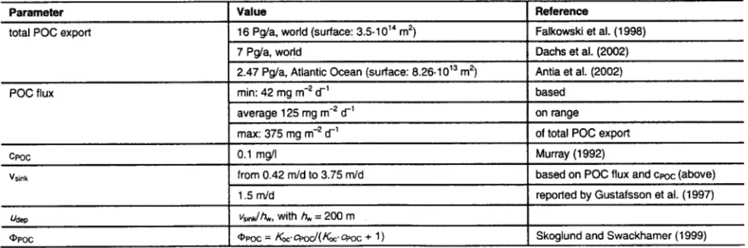
2.2 Parameterization of export to the deep sea

Export to the deep sea takes place via sorption of chemical pollutants onto particles which sink to the deeper ocean by gravitational settling. While most of the particulate organic carbon (POC) present in the surface ocean is in the form of small particles (Fowler and Knauer 1986), the export to the ocean interior of POC and associated chemicals is caused by larger aggregates, often termed 'marine snow', which have sinking velocities up to several 100 m.d -l (Alldredge and Sil- ver 1988, Alldredge and Gottschalk 1989; Pilskaln et al. 1998). The flux of POC-associated chemical, Fchem (in g-m-Z.d-1), can be written as

Fchem

= Vsink " Cpatl ( 2 )

with v,i,k denoting the average sinking velocity of the POC

(in m.d -I) and

Cp~,~

denoting the concentration of the pollut-

ant associated with particles (in g-m -3 of water). For the calculations with ChemRange, a global average of v,i,k needs to be estimated. This can be based on several sources. The approach which is likely to be most reliable on a global scale is based on the relationship between chlorophyll concentra-

tion and carbon export rate (Baines et al.

1994,

Falkowski

et al. 1998, Dachs et al. 2002). Global distributions of chlorophyll concentrations can be obtained from remote sensing data; the carbon export can then be derived from a direct relationship between chlorophyll concentration and carbon export (Baines et al. 1994) or from relationships between chlorophyll concentration and primary production and primary production and carbon export (Falkowski et al.

1998,

Eppley and Peterson

1979,

Behrenfeld and Fal- kowski 1997).

Using the latter approach, Falkowski et al. (1998) determined a global carbon export of 16 Pg POC per year, which converts into 125 mg-m-Zd -1. In combination with an average concentration of POC in the surface ocean of Cpo r = 0.1 mg.1-1 (Murray

1992), this leads to an average sinking velocity of//sink =

1.25 mJd. Using remote sensing data for the period of Octo-

ber to December

1998,

Dachs et al. (2002) estimated a total

export of POC of 7 Pg.a -1 (aggregated data from Table 1 in Dachs et al. (2002), corresponding to 60 mg.m-Z-d -1), which is about half the value reported by Falkowski et al. (1998) and corresponds to a sinking velocity of 0.60 m-d -1. Antia et al. (2002) reported a POC flux of about 80 mg.m-Z.d -1 for the Atlantic Ocean derived from POC measurements at 27 locations and correlations with primary production (calculated from Table 3 in Antia et al. (2002)).

Since the POC flux is caused by larger aggregates, it should be possible to reconcile POC flux measurements from traps moored in the deeper ocean with the flux of aggregates forming marine snow. For the euphotic zone of Monterey Bay,

(3)

POPs Series

Deap Sea Export

Pilskaln et al. (1996) reported annual mean carbon export rates of 240 mg-m-2-d -1 (based on POC flux data for the years 1989 to 1992). Compared with these data, the POC flux estimated from observations of sinking aggregates is somewhat higher; for a discussion of this discrepancy, see Pilskaln et al. (1998).

A second approach to determining POC export rates uses the disequilibrium between the natural isotope 234Th (highly particle bound) and its source 23sU (more water soluble) as a measure of particulate matter flows (Gustafsson et al. 1997). For pelagic surface waters in the Northwest Atlan- tic, Gustafsson et al. (1997) reported sinking velocities v,i.k around 1.5 m.d-L However, this figure refers only to a specific area and time and derivation of a global average from this value is fraught with uncertainty.

Based on the information from the different approaches, a

range of POC fluxes of 42 to 375 mg.m-2-d -~ is used here,

which corresponds to sinking velocities v,i,k from 0.42 to

3.75 m-d -~ (range determined by a factor of 3 around the estimate of 125 mg-m-2.d -1, which is used as a base case). Note that this average sinking velocity v,ink of POC, which is given by the ratio of POC flux and P O C concentration, is significantly lower than the actual sinking velocity of the aggregates forming marine snow because the sinking particles account only for a small fraction of the POC concentration. With an assumed depth of the surface water layer of h w = 200 m, see Fig. 1, a rate constant for POC export is obtained as Usi~ = / / s i n k / h w 9

The fraction of chemicals associated with sinking particles is calculated from the chemicals' Ko~ values (Skoglund and Swackhamer 1999) and the average POC concentration, Cvoc:

cp~ = Ka = Ko~ "cr,oc (3)

Csol

with the chemical's concentrations in the particle-bound phase, eva,, and in solution, C,ol; the dimensionless distribu-

tion coefficient Ka; the organic carbon partition coefficient

Ko~ = 0.41.Kow (in l.kg -1) (Karickhoff 1981); and Cvo c = 0.1 mg-1-1. This leads to the fraction bound to POC, ePoc, as

cp~

K d (4)

( I ) p O C - - -

-C pan + Csol Kd + 1

With c w = c_~, + c,o I, the concentration of particle-bound

chemical is t[~en cp~,~ = evoc.Cw. In the model equations, the

term u,i,k.r accounts for export of particle-bound

chemical from the surface ocean. The quantities and expres- sions used to determine the export of particle-bound chemicals to the deep sea are listed in Table 1.

2.3 Substance properties for selected PCB congeners A set of seven PCB congeners spanning a range of partition coefficients and degradation rate constants is used in the model calculations. The congeners are PCB 8, 28, 52, 101, 153, 180, and 194. Partition coefficients are taken from Li et al. (2003) and degradation rate constants are derived from half-lives reported by Wania and Daly (2002), see Table 2. The KOA values are calculated from the KAW values given in Table 2 in combination with a corrected octanol-water solu-

" ' K

bility rano, Kow=Co _.re / c , v,~. In contrast to the ow, this value is not affected'~y the'mutual solubility of octanol and water (Beyer et al. 2002). For PCBs in particular, Li et al. (2003) report a relationship

Iog[Co,purffCW, pure] = 1.16 log Kow - 0.64 (5)

for this correction. Here, the corrected KOA values are used. Another important modification of the substance properties concerns temperature. To demonstrate the effect of temperature on the model results, the substance properties were adjusted to 280 K, which is closer to the global average surface temperature. These values (Table 2, bottom) are based on temperature dependencies of the partition coefficients as reported by Li et al. (2003) and on activation energies from Anderson and Hites (1996).

Table 1: Parameters used to describe the export of particle-associated chemicals to the deep sea

Parameter Value Reference

total POC export 16 Pg/a, world (surface: 3.5-10 TM m 2) Falkowski et al. (1998)

POC flux

7 Pg/a, wodd Dachs et al. (2002)

Antia et al. (2002) 2.47 Pg/a, Atlantic Ocean (surface: 8.26-10 ~3 m 2)

min: 42 mg m -2 d -1 based

average 125 mg m -2 d -1 on range

of total POC export max: 375 mg m -2 d -~

cPoc 0.1 mg/I Murray (1992)

vsink from 0.42 rn/d to 3.75 m/d based on POC flux and cPoc (above)

1.5 rrVd reported by Gustafsson et al. (1997)

Uaep vsinuJhw, with hw = 200 m

(4)

Table 2: Partition coefficients, degradation rate constants, and particle-bound fractions in water and air of selected PCB congeners. Top: parameter values for 298 K (Wania and Daly 2002, Li et al. 2003), bottom: parameter values adjusted for 280K with activation energies from Anderson and Hites (1996) and phase transfer energies from Li et al. (2003). Second-order rate constants for reaction with OH radicals converted into first-order rate constants with OH radical concentration in air of 7.25.10 s molecules/cm3; see Wania and Daly (2003) for a discussion of this value

PCB k, k . k= log/tAw log Kow log KoA ~ r

(e-') (s -1) (a-')

(-)

(%)

8 3.50.104 6.21.10 "~ 1.05.10 "-s -2.03 5.12 7.34 0.32 0.096 28 1.93"10 "e 3.50.10 "s 7.54.10 -r -1.91 5.66 7.85 1.12 0.18 52 1.13.10 4 1.93.104 4.28.10 -7 -2.00 5.91 8.22 1.95 0.29 101 1.93.104 6.21-104 2.18.10 -r -2.01 6.33 8.73 5.05 0.56 153 3.50.10 -m 3.50.10-9 1.16-10-;' -2.10 6.87 9.44 15.5 1.36 180 1.93-10 -1~ 3.50-10 4 7.25.104 -2.48 7.16 10.16 26.3 3.31 194 1.13-10 -m 3.50.104 3.62.10 "a -2.75 7.76 11.13 58.7 10.5 8 1.61-10 -s 2.86.10 "-s 8.11.10 -7 -2.60 5.37 8.17 0.58 0.28 28 8.84-10 -s 1.61'10 -a 5.81.10 -~ -2.50 5.96 8.74 2.19 0.59 52 5.21-10 -9 8.84-10 "9 3.30.10 -7 -2.60 6.21 9.14 3.88 0.97 101 8.84-10 -~~ 2.86.10-9 1.68-10 -z -2.68 6.60 9.76 8.96 1.89 153 1.61.10 -1~ 1.61-10-9 8.95-10 -e -2.80 7.22 10.51 29.1 5.26 180 8.84.10 ~ 1.61.10-9 5.59.10 -s -3.20 7.49 11.21 43.1 11.9 194 5.21.10 -~1 1.61.10-9 2.80-10 -s -3.49 8.08 12.19 74.7 31.8

3 Model Results _lOO

r -

Model runs are performed for several scenarios. In a first "~

step, the effect of adjusting the physicochemical properties t~ ~ 80

to 280 K is investigated and then the influence of deep sea ~ "6 _o

export is demonstrated for the temperature of 280 K. The -~ ~ 60

first set of model results is for a temperature of 298 K and ~

no export to the deep sea. An example of the spatial concert- .~ E 40

tration distributions obtained from the model is given in .~ .~

Fig. 2 for the example of PCB 101. In all cases, the chemi- o . ~ o

cals are released to the air in cell / = 1; the spatial ranges are ~ o a0

calculated from the atmospheric concentration distributions

as shown in Fig. 2. 1 0 0 2 0 0

194

i " % ₎

300' 40(~ 500

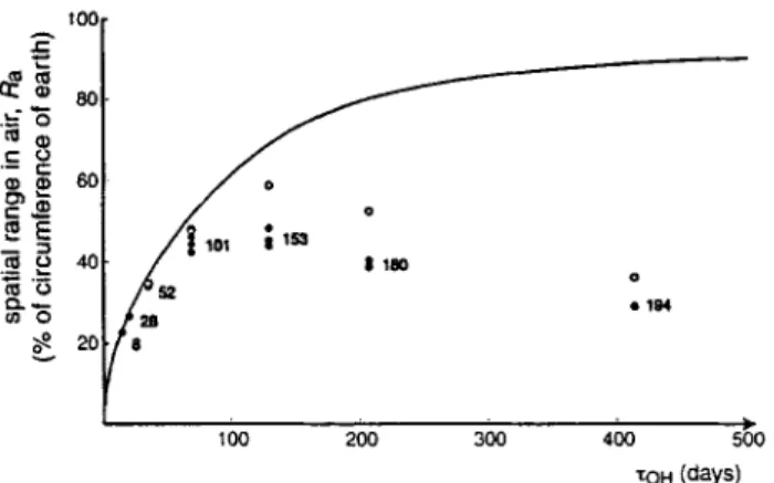
XOH (days) Fig. 3: Spatial ranges in air, Ra, of the seven PCB congeners vs. chemical lifetime in air, ZoH = l/koH for two different temperatures (298 K, open circles, and 280 K, dots). All calculations without export to the deep sea. The solid line represents the function Ra(xa) defined in Eq. 7. AXo~ is the difference between the atmospheric lifetimes of PCB 194 at 280 and 298 K

Fig. 2: Atmospheric concentration distribution and spatial range, Ra, of PCB 101 in the ChemRange model. Data for 298 K, no export to the deep sea, release into air. R a in % of the circumference of the earth

The second set of calculations is for 280 K, again without export to the deep sea. In Fig. 3, the results for the spatial ranges obtained for the two temperatures are shown as func- tions of the inverse of the O H radical reaction rate constant, Xo. = l / k o . , koH is derived from second-order rate constants for reaction with O H and an average O H radical

concentration of CON = 7.25.10 s molecules-cm -3 (Wania and Daly 2002).

The two scenarios shown in Fig. 3 indicate the effect of adjusting the chemical properties to a lower temperature. In the first scenario, data for 298 K, the spatial range increases from about 25% of the circumference of the earth for PCB 8 and PCB 28 to 65% for PCB 180 and PCB 194. Due to their long half-lives in air, the heavier PCBs have the highest spatial ranges; deposition to water and soil is not highly efficient (see below, Discussion Section).

If the chemical properties are adjusted to 280 K, the lifetimes in air, XOH = 1/koH , are higher by a factor of about 1.3 for most congeners (the activation energies are about 10 kJ/mol).

(5)

POPs Series

Deap Sea Export

1oo r - ~ 60

==_=

. ~ E ._~ 9 40

~~

2o 8 0 0 9 lg4

10o 200 ~0o 4oo 500

T O H (days) Fig. 4: Spatial ranges in air, Ra, of the seven PCB congeners vs. chemical

lifetime in air, "COB = 1/koH. Dots: Data for 280 K, with export to the deep

sea, base case and cases with low and high POC export. Circles: Results

for 280 K, without export to the deep sea (same as in Fig. 3); for congeners 8 and 28, these are neady identical to the scenarios with deep sea

export and therefore not indicated. The solid line represents the function R3(x,) defined in Eq. 7.

This corresponds to an increase from 11 d to 14 d for PCB 8 and from 320 d to 413 d for PCB 194, indicated as ~%H in Fig. 3. For the lighter congeners (8 to 52), the higher lifetime in air leads to an increase in the spatial range by a factor of 1.1. The heavier congeners, in contrast, exhibit a decrease in the spatial range because, in addition to the increase in XOH , their ~ values increase significantly and therefore also their depositional fluxes (Beyer et ai. 2003): PCB 194 has a particle-bound fraction of 30% (instead of 10% at 298 K) and PCB 180 has 12% instead of 3%. This causes a considerable reduction of their spatial ranges by a factor of 0.65 (PCB 194) and 0.85 (PCB 180).

A third set of model runs is performed with the data for 280 K and with export to the deep sea. Here, the base case of the export flux and the cases with high and low POC export were considered. The spatial ranges for these three cases are shown in Fig. 4 in combination with the results for 280 K, no deep sea export, from Fig. 3.

Comparison of the base case with the results for the case without export to the deep sea shows that transfer to the deep sea reduces the spatial ranges of congeners 101 to 194 by factors of 0.93, 0.77, 0.75, and 0.8, respectively. The highly chlorinated congeners now have spatial ranges which are compara- ble to those of the lighter ones and a maximum spatial range is obtained for intermediate congeners 101 and 153. Com- pared to this general effect, the cases with high and low POC export lead to small differences in the spatial range (less than +5% in most cases). In other words, the spatial range is relatively insensitive to changes in the depositional flux and the uncertainty of the parameterization of the deposition process does not strongly affect the results for the spatial range.

4 Discussion

4.1 Analysis of spatial ranges and mass fluxes

The model results can be interpreted by analyzing the congeners' residence time in air, '[~, which is given by the in-

verse of the effective rate constant for removal from the air, k~, see Eq. 6.

1 1

r, - - (6)

ka koH " ( 1 - ~ a ) + F ' u d e p

koH-(1 - ~ ) is the effective O H radical reaction rate constant; the factor (1 - ~ ) represents the assumption that the particle-bound fraction ~3 is not degraded (see Scheringer 2002, p. 175, for a discussion of this assumption). The term F.ud~ p is the net deposition rate constant, consisting of the overall rate constant for deposition from the air to the ground, uae p (in d -l), and the 'stickiness', F (Beyer et al. 2000). ude p depends on the dry particle deposition rate, the rain rate, the particle scavenging ratio, and the chemicals' partition coefficients. The stickiness denotes the fraction of the depositional flux that is degraded in soil or water or other- wise lost from the surface media, for example by export to the deep sea. F can vary between 0 and 1; low F indicates that a large fraction of the chemical revolatilizes, high F indicates that a large fraction is lost in the surface media. F is mainly determined by the loss processes in the surface media, but not by a chemical's partition coefficients (see below, section 4.2, for a more detailed discussion of this point). We therefore suggest the term 'net deposition factor' instead of 'stickiness' for F: the magnitude of F determines the net

deposition rate constant, F-u,~cp , as compared to the overall

deposition rate constant, ujc0, but it does not signify whether a chemical is 'sticky' in terms of a high affinity to the surface media as expressed by high Koa or low KAw.

The solid line in Figs. 3 and 4 provides a reference point for the analysis of '[3- It is the analytical relationship between the spatial range in air and '[~, which reads (Held 2001)

9 arsinh 0 05.sinh

R = 1 G

(7)

Here, D~ = 2.106 m 2 s -1 is the eddy diffusion coefficient de- scribing large-scale mixing of the atmosphere (Scheringer 1996) and G is the circumference of the earth.

In a plot of R 3 vs '[OH, as shown in Figs. 3 and 4, chemicals whose residence time in air, x3, is given by ZOH lie on this line. Deviations from the line are caused by processes leading to residence times '[3 different from '[oH- These include associa- tion with aerosol particles, expressed by the factor (1 - ~3) in Eq. 6, and net deposition to the ground, expressed by the term F.ud~ p in Eq. 6. While the factor (1 - ~3) increases "~ as

compared to '[oH, the net deposition term F'ude p decreases

z 3. If degradation or other removal processes in soil and water are slow compared to revolatilization, F is close to 0 and there is no net deposition so that '[3 is approximately given by 1/(koH- (1 - q ~ ) ) . If degradation or other losses in soil and water are fast compared to revolatilization, F approaches 1 and ud~ p describes the net deposition. In this case, '[~ depends on the relative magnitude of koH.(1 -(I)a) and ude p.

(6)

Table 3: Chemical lifetime in air, "Coil, effective OH radical reaction rate constant, koH.(1 - Oa), deposition rate constant, u~o, net deposition factor ('stickiness'), F, and atmospheric residence time, "ca, of the selected PCB congeners. Data for 280 K, without and with deposition to the deep sea (indices 'w/out' and 'with')

PCB ~OH koH.(1 -- 0.) U ~ Fwlo~ ~. we,. Fweh ~, w,h

(d) (d -~) (d -~) (-) (d) . (-) (d) 8 14.3 6.99.10 -2 7.18.10 -3 0.779 13.2 0.781 13.2 28 19.9 4.99-10 -2 7.17.10-3 0.634 18.4 0.655 18.3 52 35.1 2.83.10 -2 7,99-10-3 0.547 30.7 0.612 30.2 101 69,0 1.43.10 -2 9,33.10-3 0.355 57.1 0.617 50.1 153 129 7.33.10-3 1,35.10 -2 0.352 82.9 0.859 52.9 180 207 4.26.10-3 2.19.10 .-2 0.562 60.3 0.959 39.5 194 413 1.65.10-3 4.48.10 -2 0.797 26.7 0.992 21.7

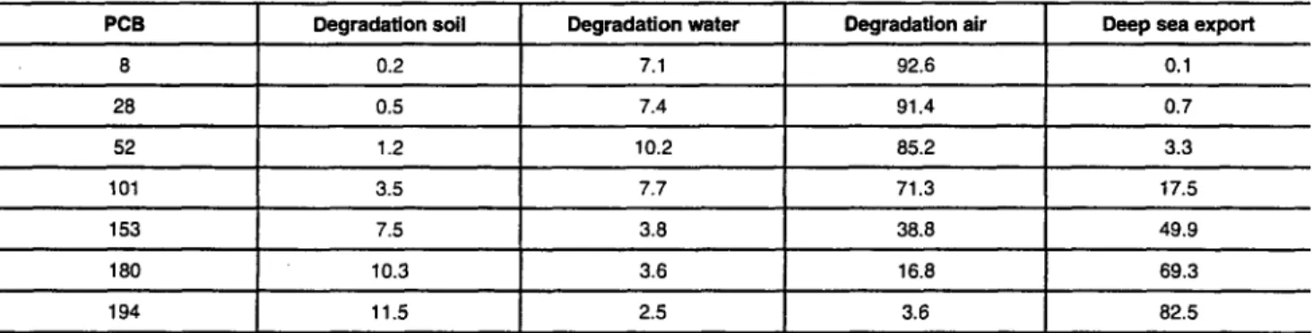
Table 4: Mass fluxes of degradation processes in all media and deep s e a export (in percent of the continuous source). Data for 280 K, export base case

PCB Degradation soil Degradation water Degradation air Deep sea export

8 0.2 7.1 92.6 0.1 28 0.5 7.4 91.4 0.7 52 1.2 10.2 85.2 3.3 101 3.5 7.7 71.3 17.5 153 7.5 3.8 38.8 49.9 180 10.3 3.6 16.8 69.3 194 11.5 2.5 3.6 82.5

In Table 3, the atmospheric lifetime ZOH = 1 / k o . , the effective OH radical reaction rate constant, koH.(1 - Oa), the

deposition rate constant Uar the net deposition factor F,

and the atmospheric residence time Xa are given for the seven PCB congeners (data for 280 K, scenarios without deep sea export and with the export base case). In the scenario without deep sea export, the net deposition factor F is almost identical for PCB 8 and PCB 194 (about 0.8) and has a minimum for PCB 153 (0.35). If export to the deep sea takes place, F has a minimum of 0.61 for PCB 52 and increases up to 0.99 for PCB 194. This represents the increase of the net deposition caused by export to the deep sea.

The figures in Table 3 show that the lighter congeners have atmospheric residence times, z~, close to the chemical lifetime, Zo8, although their net deposition factors are relatively high. Despite high F, the net deposition is ineffective compared to atmospheric degradation, because Uae p is small compared to koH-(1 - O). The heavier congeners, in contrast, h a v e Ude p values greater than koH.(1 - Oa) and, therefore, their residence times are much lower than %H, especially in combination with high F values. The value of F alone does not indicate whether or not x~ is close to ZoH but the net deposition rate constant, F.u&p, needs to be compared to the atmospheric degradation rate constant.

For the PCBs considered here, the relative magnitude of F.ud~ p and koH.(1 - 9 a) changes between congeners 101 and 153 (see Table 3). PCB 153 has F.Ude p smaller than koH-(1 - qb)

for the case without deep sea export but, because of the

high value of F = 0.859, F.Udc p greater than koH.(1 - O~) if

export takes place. For this reason, the most pronounced difference in R~ between the cases without and with export

is observed for PCB 153. PCB 101, in contrast, has F.ua, p

below ko8.(1 - Oa) for both cases, without and with export and therefore inclusion of deep sea export has a less pronounced effect. However, PCB 101 has the highest relative difference between the F values for the cases with low and high export (0.789 and 0.475, which is a factor of 1.66). For this reason, the differences between the three export cases are most pronounced for PCB 101.

The relative magnitude of net deposition and atmospheric degradation is reflected by the mass fluxes of all loss processes from the model system listed in Table 4. For PCB 101, degradation in air accounts for 71.3% and deep sea export for 17.5% of the total loss. PCB 153, in contrast, has 38.8%

loss through atmospheric degradation and 4 9 . 9 % loss

through deep sea export. Wania and Daly (2002) investigated the same suite of PCB congeners with the Globe-POP model and found a similar general pattern (deep sea export dominant loss for PCB 153 and heavier congeners, degradation in air dominant for PCB 101 and lighter congeners), although several factors are different in the two models (ide- alized vs. realistic release pattern, steady-state vs. dynamic model, no temperature influence in ChemRange).

(7)

POPs Series

Deap Sea Export

4.2 Influence of model assumptions

There are some aspects of the model results that are caused by the specific assumptions of the ChemRange model. The first one concerns the interpretation of the net deposition factor, F. The increase in/: caused by export to the deep sea (see Table 3) highlights that the value of F is not primarily determined by the partition coefficients Kow or KOA but by the removal rate constants in water and soil. PCBs 8 and 194 have similar F in spite of a difference in log Kow of three units. If the Kow of PCB 8 is increased by one order of magnitude, its net deposition factor changes only margin- ally from 0.779 to 0.794. Increase of the rate constants k s and kw by one order of magnitude, however, leads to F = 0.972. More generally, relatively volatile compounds can have high net deposition factors if they are quickly degraded in water and soil, and semivolatile compounds can have low net deposition factors if they are sufficiently persistent in water and soil.

This finding is a feature specific to steady-state models. A near-zero net deposition factor is obtained for hydrophobic, persistent chemicals because, in a steady-state model, all media are completely 'filled' with the chemical. At the be- ginning of a release period, however, when the different media have not yet achieved a state of equal inflow and outflow, the net deposition factor would be influenced not only by the degradation rate constants, but also by a chemical's affinity to the surface media, which is expressed by its partition coefficients. Under this condition, the interpretation of the net deposition factor as the 'stickiness' of the chemical would be more appropriate.

A second main point concerns the model geometry. As a general result, the finding of highest F values for the highly chlorinated PCBs (see Table 3) is consistent with F values obtained with the TaPL3 model (Beyer et al. 2000). The TaPL3 model, however, represents a continental area and contains 90% soil and 10% freshwater as surface media and its air compartment is only 1000 m high. Accordingly, the primary removal process is degradation in soil, followed by burial in freshwater sediments and degradation in freshwater. In the ChemRange model, in contrast, the ocean water dominates the properties of the surface media. Only with oceanic deposition included, the removal efficiencies of the different PCBs in the surface media and the sequence of the long-range transport potentials obtained with both models for the suite of PCB congeners are similar (Wania and Dugani 2003). In addition, the finding of lower spatial ranges for the heavier congeners, as shown in Fig. 4, is in qualitative agreement with field measurements of the distributions of different PCB congeners along south-north transects (Ocken- den et al. 1998, Meijer et al. 2002).

However, when the results from the ChemRange model are compared with other model results or field data, it should be born in mind that the model assumes identical temperature at all places. Accordingly, it does not account for the effect of varying temperature on the partitioning and degra-

dation of different PCB congeners, which strongly affects field observations and also the results of the Globo-POP model. In addition, the ChemRange model is a steady-state model and represents a situation that would be achieved only after a long time of continuous release. The model does not reflect episodic situations or concentration patterns in the period before a steady state has been achieved. The pur- pose of the ChemRange model is not to predict actual concentrations, but to illustrate effects such as the influence of deep sea export on the spatial range in a semi-quantitative way and to analyze underlying factors such as the interplay of degradation and net deposition.

5 Conclusions

The model results suggest that export to the deep sea indeed has an influence on the atmospheric tong-range transport of highly hydrophobic chemicals. As a general point, this might have been assumed from the finding that transfer to the deeper ocean is an important pathway for these compounds on a global scale (Dachs et al. 2002, Wania and Daly 2002). However, the actual magnitude of the effect can be determined only by including a realistic parameterization of the deposition process into the model. If deposition rates derived from current knowledge on organic carbon export into the ocean interior are used in the model, the spatial ranges of the congeners 153, 180, and 194 are reduced by 20 to 25%. If, in addition, the chemical properties are adjusted to a more realistic temperature of 280 K, the spatial ranges of the heaviest PCBs are similar to the spatial ranges of the lighter congeners 28 and 52. These adaptations make the model results more consistent with experimental findings suggesting that heavier PCB congeners have a lower long- range transport potential than intermediate congeners. These results underline that the long-range transport of POPs is determined by the interaction of the air with the underlying surface media and the processes taking place in these media. An additional aspect that has not been discussed here is that a certain fraction of the amount of a POP that under- goes long-range transport is transported in the ocean water (Stroebe et al. 2003). For these reasons, the long-range transport of POPs needs to be treated as a multimedia problem. The model results further imply that export to the deep sea should be considered in all models of the global distribution dynamics of POPs. Especially for compounds with Kow > 106, oceanic deposition is likely to become a relevant mass flux. Although the transfer to the deeper ocean reduces the long- range transport potential of POPs, it does not represent a true removal process. It is desirable to further elucidate the fate of POPs that have reached the deeper ocean.

References

Alldredge AL, Gottschalk CC (1989): Direct Observations of the Mass Flocculation of Diatom Blooms: Characteristics, Settling Velocities and Formation of Diatom Aggregates. Deep-Sea Res 36:159-171

(8)

Alldredge AL, Silver MW (1988): Characteristics, Dynamics and Significance of Marine Snow. Prog Oceanog 20:41-82 Anderson PN, Hites RA (1996): OH Radical Reactions: The Ma-

jor Removal Pathway for Polychlorinated Biphenyts from the Atmosphere. Environ Sci Technol 30, 1765-1763

Antia AN, Koeve W, Fischer G, Blanz T, Schulz-Bull D, Scholten J, Neuer S, Kremling K, Kuss J, Peinert R, Hebbeln D, Bathmann U, Conte M, Fehner U, Zeitzschel B (2001): Basin-wide particulate carbon flux in the Atlantic Ocean: Regional export patterns and potential for atmospheric CO 2 sequestration. Glo- bal Biogeochem Cy 15, 845-862

Baines SB, Pace ML, Karl DM (1994): Why Does the Relationship between Sinking Flux and Planktonic Primary Production Dif- fer between Lakes and Oceans? Limnol Oceanogr 39:213-226 Behrenfeld MJ, Falkowski PG (1997): Photosynthetic Rates De- rived from Satellite-Based Chlorophyll Concentration. Limnol Oceanogr 42, 1-20

Bennett DH, McKone TE, Matthies M, Kastenberg WE (1998): General Formulation of Characteristic Travel Distance for Semivolatile Organic Chemicals in a Multi-Media Environment. Environ Sci Technol 32, 4023-4030

Beyer A, Mackay D, Matthies M, Wania F, Webster E (2000): As- sessing Long-Range Transport Potential of Persistent Organic Pollutants, Environ Sci Technol 34, 699-703

Beyer A, Wania F, Gouin T, Mackay D, Matthies M (2002): Select- ing Internally Consistent Physical-Chemical Properties of Or- ganic Compounds, Environ Toxicol Chem 21,941-953 Beyer A, Wania F, Gouin T, Mackay D, Matthies M (2003) Tem-

perature Dependence of the Characteristic Travel Distance. Environ Sci Technol 37, 766-771

Dachs J, Bayona JM, Albaig6s J (1997): Spatial distribution, verti- cal profiles and budget of organochlorine compounds in West- ern Mediterranean seawater. Mar Chem 57, 313-324 Dachs J, Lohmann R, Ockenden WA, M6janelle L, Eisenreich SJ,

Jones KC (2002): Oceanic Biogeochemical Controls on Global Dynamics of Persistent Organic Pollutants. Environ Sci Technol 36, 4229-4237

Eppley RW, Peterson BJ (1979): Particulate Organic Matter Flux and Planktonic New Production in the Deep Ocean. Nature 282, 677-680

Falkowski PG, Barber RT, Smetacek V (1998): Biogeochemical Controls and Feedbacks on Ocean Primary Production. Science 281,200-206

Finizio A, Mackay D, Bidleman TF, Harner T (1997): Octanol-Air Partition Coefficient as a Predictor of Partitioning of Semivolatile Organic Chemicals to Aerosols. Atmos Environ 31,2289-2296 Fowler SW, Knauer GA (1986): Role of Large Particles in the Trans- port of Elements and Organic Compounds Through the Oce- anic Water Column. Prog Oceanog 16, 147-194

Froescheis O, Looser R, Cailliet GM, Jarman WM, Ballschmiter K (2000): The Deep-Sea as a Final Global Sink of Semivolatile Persistent Organic Pollutants? Part I: PCBs in Surface and Deep- Sea Dwelling Fish of the North and South Atlantic and the Monterey Bay Canyon (California). Chemosphere 40, 651-660 Gustafsson O, Gschwend PM, Buesseler KO (1997): Settling Re- moval Rates of PCBs into the Northwestern Atlantic Derived from 23sU-234Th Disequilibria. Environ Sci Techno131, 3544-3550 Held H. (2001): Semianalytical Spatial Ranges and Persistences of

Non-Polar Chemicals for Reaction-Diffusion Type Dynamics. In: Integrated Systems Approaches to Natural and Social Dy- namics (Eds. M. Matthies, H. Malchow, J. Kriz), Springer, Heidelberg

Karickhoff SW (1981): Semi-Empirical Estimation of Sorption of Hydrophobic Pollutants on Natural Sediments and Soils. Chemo- sphere 10, 833-846

Kr~imer W, Buchert H, Reuter U, Biscoito M, Maul DC, Le Grand G, Ballschmiter K (1984): Global Baseline Pollution Studies IX: C6-C14 Organochlorine Compounds in Surface-Water and Deep-Sea Fish from the Eastern North Atlantic. Chemosphere 13, 1255-1267

Li N, Wania F, Lei YD, Daly G (2003): A Comprehensive and Criti- cal Compilation, Evaluation and Selection of Physical Chemi- cal Property Data for Selected Polychlorinated Biphenyls. J Phys Chem Ref Data, in press

Meijer SN, Steinnes E, Ockenden WA, Jones KC (2002): Influence of Environmental Variables on the Spatial Distribution of PCBs in Norwegian and U.K. Soils: Implications for Global Cycling. Environ Sci Technol 36, 2146-2153

Murray JW (1992): The Oceans. In: Butcher SS, Charlson RJ, Orians GH, Wolfe GV (Eds.): Global Biogeochemical Cycles. Academic Press, London, 175-211

Ockenden WA, Sweetman A J, Prest HF, Steinnes E, Jones KC (1998): Toward an Understanding of the Global Atmospheric Distribu- tion of Persistent Organic Pollutants: The Use of Semipermeable Membrane Devices as Time-Integrated Passive Samplers. Environ Sci Technol 32, 2795-2803

Pilskaln CH, Paduan JB, Chavez FP, Anderson RY, Berelson WM (1996): Carbon Export and Regeneration in the Coastal Upwelling System of Monterey Bay, Central California. J Ma- rine Res 54, 114~-1178

Pilskaln CH, Lehmann C, Paduan JB, Silver MW (1998): Spatial and Temporal Dynamics in Marine Aggregate Abundance, Sink- ing Rate and Flux: Monterey Bay, Central California. Deep-Sea Res II 45, 1803-1837

Scheringer M (1996): Persistence and Spatial Range as Endpoints of an Exposure-Based Assessment of Organic Chemicals. Environ Sci Technol 30, 1652-1659

Scheringer M (2002): Persistence and Spatial Range of Environ- mental Chemicals. Wiley-VCH, Weinheim

Scheringer M, Matthies M, Hungerbiihler K (2001): The Spatial Scale of Organic Chemicals in Multimedia Fate Modeling - Re- cent Developments and Significance for Chemicals Assessment. Environ Sci Pollut Res 8, 150-155

Scheringer M, Stroebe M, Held H (2002): Chemrange 2.1 - A Mul- timedia Transport Model for Calculating Persistence and Spa- tial Range of Organic Chemicals. ETH Ziirich, Ziirich httn:// ltcmail.ethz.ch/hungerb/research/product/cbemrange.html Skoglund RS, Swackhamer DL (1999): Evidence for the Use of Or-

ganic Carbon as the Sorbing Matrix in the Modeling of PCB Ac- cumulation in Phytoplankton. Environ Sci Technol 33:1516-1519 Stroebe M, Scheringer M, Held H, Hungerb/ihler K (2003): Inter- Comparison of Multimedia Modeling Approaches: Modes of Transport, Measures of Long Range Transport Potential and the Spatial Remote State. Sci Total Environ, in press

Wania F, Daly G (2002): Estimating the Contribution of Degrada- tion in Air and Deposition to the Deep Sea to the Global Loss of PCBs. Atmos Environ 36, 5581-5593

Wania F, Dugani C (2003): Assessing the Long-Range Transport Potential of Polybrominated Diphenyl Ethers: A Comparison of Four Multimedia Models, Environ. Toxicol. Chem. 22, 1252-1261

Received: March 10th, 2003 Accepted: October 29th, 2003