Depth and orbital tuning : a new chronology of glaciation and nonlinear orbital climate change

Depth and Orbital Tuning:

Glaciation and Nonlinear Orbital Climate Change.

by

Peter Huybers

Submitted to the Department of Earth, Atmospheric, and Planetary

Sciences

in partial fulfillment of the requirements for the degree of

Master of Science in Climate Physics and Chemistry

at the

MASSACHUSETTS INSTITUTE OF TECHNOLOGY

May 2002

@

Peter Huybers, MMII. All rights reserved.

The author hereby grants to MIT permission to reproduce and

distribute publicly paper and electronic copies of this thesis document

in whole or in part.

Author ...

Department of Earth, Atmosphr ,

....

.. ... -.

...

and Planetar Sciences

II

M 18, 2002

Certified by...

Carl Wunsch

Director, Program in

mosp e

Oceans, and Climate

Thesis Supervisor

Accepted by...

Ronald Prinn

d Department of Earth Atmospheric and Planetary Sciences

ES

MASSACHUSETTS INSTITute

I

_{J L .*V 't}

~JULM

Depth and Orbital Tuning: a New Chronology of Glaciation

and Nonlinear Orbital Climate Change.

by

Peter Huybers

Submitted to the Department of Earth, Atmospheric, and Planetary Sciences on May 18, 2002, in partial fulfillment of the

requirements for the degree of

Master of Science in Climate Physics and Chemistry

Abstract

It is suggested that orbital tuning casts a false light upon the chronology of glaciation and the understanding of the climatic response to orbital variations. By developing a new age-model, independent of orbital assumptions, a significant non-linear response to orbital forcing becomes evident in the 6180 record. The new age-model also indi-cates glacial terminations two through eight are 8,000 years older than the orbitally based estimates. A simple obliquity threshold model is presented which reproduces the timing, amplitude, and observed non-linearities of the 6180 record; and supports the plausibility of the new age-model and the inferred non-linear climatic response.

Thesis Supervisor: Carl Wunsch

Acknowledgments

I thank Carl Wunsch for being both an advisor and mentor. I also thank Ed Boyle,

Bill Curry, Jerry McManus, Delia Oppo, and Maureen Raymo for making much of the data available to me and for invaluable discussion and comments. This work was supported by the National Defense Science and Engineering Graduate Fellowship Program.

Contents

1 Orbitally-tuned Age-models 13

1.1 Simple Model of Sediment Accumulation . . . . 13

1.2 Orbital Parameters and Modulation . . . . 14

1.2.1 Amplitude and Frequency Modulation . . . . 14

1.2.2 Eccentricity . . . . 17 1.2.3 O bliquity . . . . 17 1.2.4 Precession . . . . 18 1.3 Orbitally-Tuned Noise . . . . 20 1.3.1 W hite Noise . . . . 22 1.3.2 R ed N oise . . . . 24

1.4 Monte Carlo Test of Orbital-Tuning . . . . 25

1.4.1 Number of Adjustable Age Control Points . . . . 25

1.4.2 Brunhes-Matuyama Age . . . . 27

1.4.3 Detailed Age-model Corrections . . . . 29

2 Depth-Tuned Age-models 33 2.1 The 6180 Records . . . . 34

2.2 Building a Depth-Tuned Age-Model . . . . 36

2.2.1 Linear Age-Depth Model . . . . 37

2.2.2 Visual Event Correlation . . . . 38

2.2.3 Automated Record Correlation . . . . 41

2.3 Monte Carlo Test of Depth-Tuning . . . . 44

2.3.1 Coherent and Incoherent 610 Energy . . . . 45

2.3.2 Skill in Correlating 6180 Records . . . . 48

2.3.3 Estimate of the True Coherent 6180 Energy . . . . 49

2.4.1 Accumulation Rate Anomalies . . . . 52

2.4.2 Mean Accumulation Rate . . . . 53

2.5 Spatial Correlation of Sediment Accumulation . . . . 57

2.6 Age-Model Uncertainties . . . . 61

2.6.1 Synchroneity of Events . . . . 61

2.6.2 Uncertainties Due to Jitter . . . . 62

2.6.3 Systematic Errors . . . . 65

2.7 Comparing the Orbital and Depth-tuned Age-models . . . . 69

2.7.1 Orbital-tuning of ODP677 . . . . 72

2.7.2 Radiometric Dates . . . . 73

3 Non-Linear Responses to Orbital Forcing. 81 3.1 Depth-tuned 6180 Record . . . . 83

3.1.1 Spectral Description . . . . 83

3.1.2 Estimating the True Spectra . . . . 85

3.1.3 The Time Rate of Change . . . . 88

3.2 Non-linear Coupling of Obliquity and the quasi-100KY Band . . . . . 90

3.2.1 Bi-linear Coupling . . . . 90

3.2.2 Non-linearities in the Vostok Spectra . . . . 92

3.3 Speculation on the quasi-100KY Glacial Cycle . . . . 93

3.3.1 Re-tuning Imbrie and Imbrie's Ice-Volume Model . . . . 93

3.3.2 Simple Models of the quasi-100KY Cycle . . . . 96

3.3.3 Threshold Model of Glaciation . . . . 100

A The XCM Tuning Algorithm 109

Introduction

Much of the process of inference concerning past climate relies heavily upon the assignment of ages to measurements and events recorded in deep-sea and ice cores. Sediment and ice accumulation are analogous to strip-chart recorders, marking the record of the past climate state in a large variety of physical variables. These records tend to be noisy and blurred by bioturbation and a variety of diffusive processes [e.g. Pestiaux and Berger, 1984]. The major difficulty, however, is that these strip-chart recorders run at irregular rates, stretching and squeezing the apparent time scale, and so distorting the signals being sought if depth in the core is taken to be linearly related to time. It is not an exaggeration to say that understanding and removing these age-depth (or 'age-model') errors is one of the most important of all problems facing the paleoclimate community, as the accuracy of such models is crucial to understanding both the nature of climate variability and underlies any serious hope of understanding cause and effect.

Orbital-tuning assumes a constant phase relationship between paleo-climatic mea-surements and an orbital forcing based on Milankovitch theory [Milankovitch, 1941], and is the currently favored method by which Pleistocene age is estimated [e.g. Imbrie 1984, Martinson 1987, Bassinot 1994, and Kent 1999]. The presence of eccentricity-like amplitude modulation in the precession band of orbitally-tuned 6180 records seems to be the clinching argument for orbital-tuning [e.g. Imbrie, 1984 and Shack-leton, 1995]. But contrary to the assertion that orbital-tuning does not affect am-plitude modulation [Paillard, 2001], the precession parameter is shown to undergo strong frequency modulation during times of low eccentricity, which when narrow-pass-band filtered, produces eccentricity-like amplitude modulation. Since the pre-cession band accounts for only a small part of the total 6180 variance [Wunsch, 2002], the narrow-pass-band filtering is necessary, and orbital tuning assures the presence of eccentricity-like amplitude modulation. This non-verification of orbital age-models is emphasized by showing orbitally-tuned noise meets the criteria [Bruggerman, 1992] for an accurately tuned 6180 record. Tuning is accomplished here by a new objec-tive algorithm termed XCM which seeks a maximum cross-correlation between two records. Having shown that post-orbital-tuning analysis of a record cannot verify an age-model, a Monte Carlo test is introduced which instead estimates the expected skill of an orbital-tuning procedure. XCM demonstrates some skill in correcting system-atic age-model errors in linear age-depth relationships (e.g. an under-estimated mean

sediment accumulation rate), but no skill in making detailed age-model corrections (e.g. correcting for random fluctuations in accumulation rate).

An alternative to orbital-tuning is to estimate age using mean sediment accu-mulation rates [Shaw, 1964, and is termed depth-tuning. The literature has numer-ous examples of depth-tuning [e.g. Shackleton and Opdyke 1972, Hays et al 1976, Williams 1988, Martinson et al 1987, and Raymo, 1997], but in each case the au-thors ultimately deem an orbitally-tuned age-model as more accurate. This uniform preference for orbital age-models reflects a confidence in the Milankovitch theory, but this theory has has recently come under question [e.g. Winograd 1992, Muller and MacDonald 1997, and Henderson and Slowey 2000, Elkibi 2001, Gallup 2002, and

Wunsch, 2002]. Compared to previous depth-tuned age-models this study benefits from a significantly greater number of V150 records (26 vs. 11 as the previous largest [Raymo, 1997]) and an analysis of sediment compaction with a correction for it at-tendant effects. Relative to orbital age-models, the depth-tuned age-model indicates terminations two through eight are each eight KY older, a conclusion supported by the available radiometric constraints on termination ages [e.g. Karner and Marra

1998, Esat et al 1999, Henderson and Slowey 2000, and Gallup 2002]. The

develop-ment of a stochastic sedidevelop-ment accumulation model allows for a Monte Carlo test of the depth-tuning procedure and provides uncertainty estimates for the depth-tuned age-model. The depth-tuned age-model has an average estimated uncertainty of 8.5KY for any individual date and it is unlikely that the systematic offset between orbital and depth-tuned ages is a result of sediment accumulation rate variations. Also, an empirical orthogonal functions (EOF) analysis of accumulation rates demonstrates basin-wide spatial patterns which are themselves of climatic significance.

Spectral analysis of the 6180 record, using the new depth-tuned age-model, indi-cates that significant energy is concentrated at

1 n

f(n)=

41 100

and at the 1/1OOKY frequency band where 1/41KY represents the obliquity band. For the leading EOF of the 26 6180 record, each spectral peak at f(n) is above of the 95% confidence level and together they account for more than 60% of the total variance. These same frequency bands display significant auto-bicoherency which strongly indicates a non-linear coupling between the 1/41KY obliquity variations and the quasi-1/100KY oscillation. A Monte Carlo spectral simulation indicates only 23% of 6180 variance is linearly attributable to obliquity and precession and, by inference,

the majority of the orbital response is non-linear. The new depth-tuned age-model is also used to re-estimate parameters for Imbrie and Imbrie's [1980] ice-volume. The re-tuned ice-volume model indicates the presence of stronger obliquity forcing and a more rapid glacial melt response, and while the model reproduces the depth-tuned timing of glaciations, the amplitudes are incorrect.

The apparent non-linear coupling between obliquity and the 1/100KY cycle mo-tivates the construction of a simple obliquity based threshold model of glaciation. The model has three adjustable parameters which set the accumulation rate, melt rate, and initial ice volume; it also successfully reproduces the depth-tuned timing of terminations, approximate amplitude of each termination, spectral peaks at f(n) and 1/1OOKY, and the observed auto-bicoherence pattern. Relative to other sim-ple climate models, this model achieves a high squared cross-correlation (0.63) with the 6180 observations using few adjustable parameters. The fidelity with which this model reproduces the salient features of the 6180 observations supports both the plausibility of the depth-tuned age-model and the inferences of non-linear climatic behavior.

Chapter 1

Orbitally-tuned Age-models

1.1

Simple Model of Sediment Accumulation

Orbital-tuning refers to the process of assigning an age to a record based on an as-sumed relationship with the earth's orbital variations. In marine sediment cores where records are initially measured against depth, orbital-tuning is, in effect, estimating sediment accumulation rates1. Beginning with the supposition that sediment accu-mulation is stochastic, the age-depth relationship can be modeled as a random walk process. Let dt be the accumulated sediment (the "depth" ) in a core at time t. t is to be regarded as a discrete variable. Then per unit time, At, dt increases at the mean sediment accumulation rate (S) plus an anomaly (S'),

dt+₁ = dt

+

Dividing by S converts the depth increment to a true time increment plus an anomaly,

n1= n~ + At + At-=.(1)

S

If S' is a stochastic variable of zero mean, and variance ou, then Eq. (1.1) rep-resents a random walk in the time variable. The simplest such model is one of uncorrelated increments, < S, >= 0, t f t'. (We use the brackets, < -> to denote expected value.) Then, the variance of the difference between the apparent and true time grows linearly on average [Feller, 1966],

1Post-deposition processes and core recovery effects are considered in more detail later in this

< (t' - nt) 2 >=

nAt--n S2

Following Moore and Thomson (1991) and Wunsch (2000), we term the rate of growth the jitter,

J _- (1.2)

S2

By permitting S' to take on more interesting temporal covariances, one can

gen-erate very complex behavior in the statistics of tn, but in the interests of simplicity, the discussion is initially confined to this basic case. The purpose of the paper is to investigate how to best infer t from measurements in t' and then to apply the results to the observed 6180 record.

1.2

Orbital Parameters and Modulation

Following the demonstration by Hays et al. (1976) of the apparent presence of Mi-lankovitch band spectral features in deep-sea cores, the plausible assumption has been made that such features are present in most climate records. Along with certain further simple assumptions, such as that of a fixed phase response to Milankovitch forcing throughout the core duration, tuning the records so as to sharpen and enhance the Milankovitch frequency bands has become the favored method to recover t (t'). We thus begin by reviewing some of the basic structure of the Milankovitch forcing.

The eccentricity, obliquity, and precessional earth orbital parameters along with the solar constant and the mean earth-sun distance are sufficient to calculate the solar radiation incident at the top of the earth's atmosphere for any given time and place. Apart from some weak secular terms, this insolation can be well approximated by a finite number of interacting periodic terms [e.g. Berger and Loutre, 1991]. These in-teractions involve only products of sinusoids, and we pause to recall the basic elements of amplitude (AM) and frequency modulation (FM).

1.2.1

Amplitude and Frequency Modulation

Consider a pure cosine, cos(27rtfi), of "carrier "frequency fi multiplied by another cosine of frequency f2. Then,

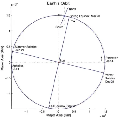
Earth's Orbit 0.5 Summer Solstice E Jun 21 Perihelion 0 .- --- . ..-.- ..- -..-.- . S ...--- u u:J ... . . . . .. a n 4 0 . Aphelion Jul 4 .Winter -0.5- Solstice Dec 21 -1-all Equinox, Se -1 -0.5 0 0.5 1 1.5 Major Axis (Km) _X 108

Figure 1-1: The current orbital configuration of the earth viewed looking downward on the North Pole. The solid line is earth's slightly eccentric orbital path (to scale), and the dotted line is a circle centered on the sun. Note that the earth is furthest from the sun during northern hemisphere summer. The earth and elliptic axis are both moving counter-clockwise, while the equinoxes and solstices are moving clockwise.

p(t) = cos(27rtfi) cos(27rtf2) = cos(27rt(fi + f2)) + cos(27rt(f1 - f2)) (1.3)

here the carrier frequency, fi, is split into two new frequencies, fi ± f2, in the process

known as amplitude modulation. A power spectrum of p (t) would display peaks not at fi, but at (fi ± f2), that is, with two-sidebands.

If instead a cosine is "frequency modulated" by another cosine we have.

p(t) = cos(27rtfi + 27r6 cos(27rtf2))

= cos(27rtfi) cos(27r6 cos(27rtf₂)) + sin(27rtfi) sin(27ro cos(27rtf₂)). (1.4)

Using a simple identity [Olver 1962, Eqs 9.1.44-45] Eq. (1.4) is,

Eccentricity ooo1 2 010-4 -0-2.6 100 102 0.03 0.015 10o 04 0.01 005 24-5 102 23-3 22.1 W*WN*V* 2.5 100 0.64 10-2 0.0281 0.025 0.02 10-4 0.01 0-05 Prece ssicn 10 2.6 1-2: 10 1 .3 0.0521-0.077 1 0-049 0-02 ~104A 120011001000900 800 700 600 500 400 300 200 100 0.01 0.05

Trime (Klyrs 13P) Prequency (1/Klyrs B3P)

Figure 1-2: Each orbital parameter is shown along with its amplitude modulation (middle), frequency modulation (bottom), and power density spectrum (right). For obliquity the orbital inclination is plotted along with the AM (dotted middle). By definition the AM of the precession parameter is eccentricity. Note in the power density spectrums that each parameter is largely confined to a unique frequency band.

00

p(t)= cos(2rtfi)[J, (276f2) + 2 E J2k (27r6f 2) cos(47ktf2)]

k=1

00

- sin(27rtfi) 1k J2k+1 (27r6fi) cos(27r(2k + 1)tf2) (1.5)

k=O

where the J, are Bessel functions. Now m(t) has spectral peaks at fi ± nf2 for n = [0,1,

2...}

1.2.2

Eccentricity

A diagram of earth's present orbital configuration is shown in Figure 1-1. The solid

ellipse shows earth's current slightly eccentric orbit to scale, while the dashed line is a circle centered on the sun. Eccentricity is measured as

L 2

e= I major (1.6)

Lminor

where L represents the length of the major and minor orbital axis. Currently the eccentricity of the earth is .01672. This produces a 7% annual change in the insolation incident at the top of the atmosphere from 354 (aphelion) to 3 3 1wts (perihelion).

This difference is primarily due to the sun's displacement from the geometric center of the earth's orbit to one of the two foci of the orbital ellipse. Eccentricity is unique among the orbital parameters in that it affects the total insolation incident on the earth rather than only redistributing it.

Figure 1-2 shows the frequency modulation and amplitude modulation of each orbital parameter [see Berger and Loutre, 1991] along with its power density spec-trum. Eccentricity, e, displays rapid transitions in frequency and amplitude at its local minima. While e is dominated by a few low-frequency terms, it also has a sig-nificant broadband component. Note however, that on these timescales, the orbital parameters are deterministic, and the frequency domain behavior of e is not that or red-noise process. This stochastic (broadband spectrum) behavior has to be included in any discussion of the effects of eccentricity on climate.

1.2.3

Obliquity

Obliquity measures the angle between earth's equatorial and orbital planes and is currently 23.50. The earth's equatorial plane precesses with a period of 25.8KY and the earth's orbital plane precesses with a period of 70KY. Obliquity measures the difference between these two planes which results in a primary insolation frequency of 1/25.8 - 1/70 = 1/41KY [see Muller and MacDonald, 2000]. Apart from the 7% change in insolation due to eccentricity and timed by precession, obliquity accounts

for the magnitude of the seasonal insolation variations.

Obliquity AM (ranging from 2.40 to 0.70) is primarily caused by variations in the inclination of the orbital plane which, measured relative to the invariant plane 2,

2

has a red noise spectrum dominated by a 1/100KY peak. Muller and MacDonald,

[1997] have proposed that the periodic alignment of the earth's orbital plane with

a galactic plane of dust could provide a physical link to the quasi-100KY glacial oscillation. Obliquity FM has a red noise spectrum dominated by two peaks at 1/170 and 1/100KY [see Liu and Chao, 1998]. Liu [1998] propose that variations in the time integrated insolation forcing due to FM accounts for the 100KY glacial oscillation. The result of these AM and FM modulations on the spectrum of obliquity is evident in the minor side-lobes flanking the central 1/41KY peak.

1.2.4

Precession

The earth precesses because of the torque exerted on its equatorial bulge by the moon and sun. This precession is nearly periodic at 25.8KY. In Milankovitch theory, however, one is interested in the climatic effect of precession which is to shift the phase of the longitude of perihelion relative to the seasonal cycle. Measuring the degree of alignment of the line of apsides with the spring equinox, and scaling by the degree of eccentricity provides a measure of the precessional influence on seasonal insolation changes. The climatic precession parameter is accordingly defined as

p(t) = e(t) sin(w(t))

where e(t) is the eccentricity, and w(t) is the angle between perihelion and the spring equinox. Climatic precession does not affect yearly mean insolation, and a model with seasonal sensitivity to insolation forcing is necessary to elicit a precessional response [see Rubincam, 1994]. Precession is elicited in Milankovitch theory by relating the glacial configuration to northern hemisphere summer insolation.

Over the last 800KY the mean frequency of the precession parameter, dfi'/dt, has been 1/20.4KY with lows in instantaneous frequency reaching 1/50KY and highs of 1/13KY. These dramatic excursions from the mean frequency are due to rapid changes in the longitude of perihelion which can be understood by considering a perturbation, F = Ri + Nh + Th x i, applied impulsively to the earth. The relevant vector components of F are i pointing from the sun to the earth and h perpendicular to the orbital plane, and the resultant change in the longitude of perihelion is [e.g.

Danby, Eq. 11.5.11, 1992]

dw = V ae

jP-Rdt

nae 1-I+ ecosv

where n is earth's average orbital angular velocity, v is the angle between perihelion and the earth, and a is earth's mean distance from the sun. The equation is valid over at least the last 5Ma as eccentricity is always greater than zero. Only those components of the impulse in the orbital plane (R and T) act to change w. Clearly the longitude of perihelion is more susceptible to perturbations when e is small and, accordingly, Figure 1-2 shows the largest excursion in dw/dt, or frequency, when eccentricity is near zero. These large variations in the frequency of precession are important for understanding why precessional amplitude modulation does not indi-cate an accurately orbitally-tuned age-model. Major causes of these perturbations to earth's orbit are Jupiter since it is massive, and Venus because it is close [Muller and MacDonald, 2000]. The time average mean of dw/dt over the last 800KY is 1/25.8-1/20.4=1/98KY, where perihelion tends to move in the opposite direction of the spring equinox.

Figure 1-3 shows the time series and power density spectra of the non-AM signal, p(t)/e(t), and that the characteristic triplet of precessional peaks is generated by FM alone. From Eq 1.3, one expects multiplication by e(t) to result in a splitting of the triplet of precessional carrier frequencies into a multitude of side-lobes. A peculiar relationship between the AM and FM of precession, however, suppresses these side-lobes as evidenced in the PSD of p(t). To gain insight into this filtering effect note that the triplet of eccentricity frequencies equals the differences of the triplet of precessional frequencies.

fP1 23.7 fP2 22.4 1 fP3 19.0 fei 4 042 -1f1 fe2 = = fP3 -fp2 fe3 98.7 fp3 -fpl

where the subscripts p and e refer to the precessional and eccentricity frequencies. Considering only the dominant triplets, the precession parameter may be written as

p(t) [sin(27t(fp2 -

fri)

[sin(27rtfp1 + #p1)

+

The ensuing sum and difference frequencies from these multiple AM relationships produce side-lobes coincident with the original precessional triplet of frequencies. For example fpi t (fp2 -

fri)

frequency and amplitude modulation are arranged to cancel one another out, and this effect is observed regardless of which period between zero and five Ma BP is chosen. The suppression of energy outside of the main triplet of precessional frequen-cies is tantamount to narrow band-pass filtering. Indeed, when comparing the PSD of p(t) with a boxcar pass-band filtered version of p(t)/e(t) (bottom of Figure 1-3) it appears the interaction of the FM and AM better suppress the energy outside of the precessional triplet than the boxcar filter itself. It is not surprising, then, that a narrow band-passed precession-like FM signal exhibits amplitude modulation similar to eccentricity.

An alternative description of the generation of precession-like AM is that, as indicated by Eq 1.7, during minima in eccentricity there are large excursions in pre-cessional frequency. Pass-band filtering diminishes the energy at these excursional frequencies, which translates into a decreased amplitude during periods of low eccen-tricity. As such, any pass-band filter can generate a precession like AM signal from a precession-like FM signal. In the next section it is shown that orbital-tuning can transform noise into a precession-like FM signal, and after pass-band filtering over the precessional triplet, the tuned noise displays precession-like AM.

1.3

Orbitally-Tuned Noise

The last section described insolation as a frequency and amplitude modulated set of carriers. If climate linearly responds to insolation variations, one would expect the modulation structure of the forcing to be at least qualitatively mimicked in the response. A multitude of methods have been used to orbitally-tune paleo-climatic records to the assumed linear insolation response. The criteria used to assess the ac-curacy of an orbitally-tuned timescale are outlined by Imbrie et al [1984] , Bruggerman

[1992] , and Shackleton et al [1995]. Generally these criteria are that geochronolog-ical data should be respected within their estimated accuracies, sedimentation rates

sin(w) 0.07 0.048 _dw/dt 0.025 Filtered sin(w) e sin(w) 800 600 400 200 0 0.02 0.04 0.06 0.08

Time (Kyrs BP) Freqeuncy (1/Kyrs)

Figure 1-3: The precession parameter divided by eccentricity and its associated PSD, (top sin w). The instantaneous frequency estimate (dw/dt in 1/KY) is shown along with the cut-off frequencies of a pass-band filter (horizontal dotted black lines and vertical in the PSD). Applying this pass-band filter results in an amplitude modulated signal (Filtered sin w) which is very similar to the precession parameter (e sin w). Note that large frequency excursions in w occur when eccentricity is small, and extend beyond the cut-off frequencies. The AM of the filtered FM signal, then, corresponds to the eccentricity AM precession parameter. Also note that the side-bands in the

PSD of e sin w drop off more quickly than the filtered signal itself; eccentricity is

effectively pass-band filtering sin w.

remain plausible, variance should become concentrated at the Milankovitch frequen-cies with a high coherency between the orbital signal and the data, and what seems to be the clinching argument, similar amplitude modulation should appear in the Milankovitch-derived insolation and in the tuned result. Imbrie et al [1984] asserted that the "statistical evidence of a close relationship between the time-varying am-plitudes of orbital forcing and the time-varying amam-plitudes of the isotopic response implies that orbital variations are the main external cause of the succession of late Pleistocene ice ages." More recently Shackleton et al [1995] concludes, "Probably the most important feature through which the orbital imprint may be unambiguously recognized in ancient geological records is the amplitude modulation of the

preces-sion component by the varying eccentricity of the Earth orbit." These assertions take on the air of accepted truths as Paillard [2001] states in comparing a band-passed

SPECMAP record with precession, "It is remarkable that both time series have a

quite similar modulation of their amplitude. This is probably one of the strongest ar-guments in favor of a simple causal relationship between the precessional forcing and the climatic response in this frequency band. Indeed, in contrast to other techniques, amplitude modulation is not affected by tuning."This section examines the degree to which apparent consistency of amplitude modulation can in fact be assumed to demonstrate accuracy in a tuned age-model.

Tuning of core data against insolation curves has been done in a number of different ways, ranging from subjective methods [Imbrie et al, 1984] to more objective methods

[Martinson et al, 1987]. Here, a simple and repeatable algorithm is used for objective tuning, but which is readily demonstrated to transform a pure noise process into one with an apparent orbitally dominated signal. In common with most such methods [e.g. Martinson, 1982 and Bruggerman, 1992], the algorithm can be used to enhance the orbital features of a record. The procedure used here is to maximize the cross-correlation between two records and is termed XCM (cross-cross-correlation maximizer)

3. XCM begins with a noise process, to be defined-below, 7(t'), and an

orbitally-based target record, T(t). For convenience, both are assumed to have zero

time-mean. A spurious assumption is made that adjustments to t' which increase the cross-correlation between T(t') and T(t) indicates an improved age-model. The adjustments

to t' take the form of a time adjustment function, y, such that ideally t' + p(t') = t. At the end of the optimization, r2 _{typically increases from near zero to about 0.25.}

See Appendix A for a detailed explanation of the XCM routine.

1.3.1

White Noise

A typical realization of XCM tuning is presented in Figure 1-4. Pure white noise, i7(t'),

is tuned to the precession parameter [Berger and Loutre, 1992], T(t)-= p, over a 800KY

period. Consistent with the results of Neeman [1993], a squared cross-correlation of

0.19 is achieved, a concentration of variance at the triplet of precessional peaks occurs,

a coherency in the precession band of greater than 0.9 is achieved (0.65 is the approx-imate 95% level of no significance), and both AM and FM similar to the precession

3

800 600 400 200 0

Time (Kyrs BP) _{Frequency (1 /Kyrs)}10-1

Figure 1-4: By tuning white noise to the precession parameter, the squared cross-correlation was increased from zero to 0.19. On the left are time series of (top) white noise, (middle) white noise tuned to precession (thin) and superimposed on the precession parameter (thick), and (bottom) tuned noise pass-band filtered over the precession band (thin) and again superimposed on the precession parameter (thick). The right shows the power density spectra (PSD) associated with each modification of the noise.

parameter has appeared-completely spuriously. This result should not be a sur-prise; attempts to maximize the correlation between two records necessarily requires the amplitudes of variations to be brought into alignment, and imposes common fre-quency modulations. The combination of these imposed amplitude and frefre-quency modulations, when pass band filtered, produces a visual amplitude modulation in the two series.

In the tuning done in this paper the sediment accumulation rates are constrained to remain within plausible levels of variation by requiring a record to never be squeezed or stretched by more than a factor of five. Considering the difficulty of determining geochronological dates in the interval between termination two (approx-imately 130KYBP) and the Brunhes-Matuyama (B-M) boundary (approx(approx-imately 780KYBP), it seems unlikely the available geochronological constraints would con-flict with this tuned age-model.

precession band

WW1AP4v4ftv\

800 600 400 200 0 0.01 0.025 0.05

Time (Kyrs BP) Frequency (1 /Kyrs)

Figure 1-5: Red noise orbitally-tuned to summer insolation at 65' North. In this case the squared cross-correlation was increased from zero to 0.31. The band-passed filtered record is shown for the precessional and obliquity bands superimposed on the

respective orbital parameters. The associated PSD are shown to the right.

1.3.2

Red Noise

Figure 1-5 shows a second tuning realization where a q(t') of red noise is tuned to a T(t) of insolation at 65 North on July 15th [Berger and Loutre, 1992]. 7(t') is

characterized by a power density spectrum, 1

f

₁₀₀₂

<D(f) has a -2 power law relationship giving way to white noise at frequencies be-low 1/100KY. This spectral relationship approximates the background continuum observed in the 6180 [see Section 2.3.1]4. The variance in T(t) is composed of 13% obliquity, 84% precession, and because the insolation is calculated for a fixed date, only .02% eccentricity. Orbital-tuning increases the squared cross-correlation from zero to 0.31. Again high coherencies and a concentration of variance are observed at

4_{For a discussion of the significance of power law relationships to the 6180 record see Shackleton} and Imbrie [1990].

the orbital frequencies. This indicates that regardless of the true nature of the 6180

record, orbital-tuning will generate an orbital-like behavior.

1.4

Monte Carlo Test of Orbital-Tuning

This section seeks to statistically characterize the capacity of tuning to increase the accuracy of an age-model when an orbital signal is present. The method adopted is to generate a synthetic record composed of an orbital-like signal and noise, jitter the

age-model of the record (this process is fully explained in Chapter 2), orbitally tune the jittered record to the original orbital-like signal, and assess the accuracy of the new age-model. While many orbitally-tuned records are reported with uncertainties, these seem to be based on subjective judgments [e.g. Imbrie et al, 1984]. The method presented here provides a more objective basis by which to estimate age-model accuracy.

The root mean square (rms) deviation of the age-model from the true-age is used to measure the accuracy,

orms () = (ti - m)2

i=0

where N is the number of data points, ti is the true age of the i - th data point, and m is the modeled age. Successful tuning is defined as,

orms (t' + p(t')) < 1, (1.9)

Urms (t)

that is, the rms deviation of the tuned age-model (t' + I(t')) from true time is less than the un-tuned age-model t'. The algorithm introduced in the preceding section is used to make a piecewise estimate of p(t'). Increasing squared cross-correlation from

Eq A apparently satisfies the outlined spectral criteria for a successful tuning. This

exercise is an attempt to see to what extent and under what conditions increasing cross-correlation indicates a more accurate age-model, i.e.

2 1

rms(t' + Pb(t'))

1.4.1

Number of Adjustable Age Control Points

Define an age control point (ACP) as a depth (dk) whose associated age can be adjusted backward and forward in time (tk = t' + pk(t')). An ACP represents a

0.25 -S200 0.2-0 400-0 .1 5 - -.. . . .. . . . .-. ---. .. . . -t 0.1- 600 t -- h(t') . .. ,800 10 20 30 40 50 800 600 400 200 0

Number of Control Points Age Model (Kyrs BP)

T(t) -S(h(t'))

0 100 200 300 400 500 600 700 800

Age (Kyrs BP)

Figure 1-6:

4'(t')

30 ACPs, 0(t' + p (t')30), and the target record, T(t), are shown at the bottom. Note

that while the tuned age-model yields a strong correlation, it is in fact significantly wrong.

degree of freedom in the age-model, but since sediment accumulation is assumed to be a monotonic process, ACPs are constrained to never reverse order. Between ACPs, time is linearly interpolated with depth; thus ACPs are points in time where the slope of (p(t')) may change. In order to recover the true time from a jittered record, assuming accumulation rates vary at all timescales, it would be necessary to assign an ACP to every measurement. But such a large number of degrees freedom coupled with the presence of noise, makes it likely that spurious features would then be correlated. Figure 1-6 shows a signal

4'(t) = v5rq(t) + v5(0(t) + p(t))

comprised of red noise q(t), obliquity 0(t), and precession p(t). 0(t) is jittered to

O(t') and correlated to T(t) = 0(t) +p(t) with three to 50 ACPs using XCM. The true

over-correlated. In this case, the age-model algorithm converges on an age-model t' + pu(t') that is worse than the original linear age-depth estimate, t'.

Because the jittered signal is aliased over the entire frequency range, the signal-to-noise ratio cannot be reliably increased. The tendency for tuning to correlate signal-to-noise can be mitigated by reducing the degrees of freedom available to the age transfer function, p(t'), and thus a small number of ACPs are used in the following exam-ples. p(t') represents a a linear piecewise adjustment to t'. It should be noted that since bioturbational effects, phase lags, and non-linear responses are excluded, these examples discuss tuning under ideal circumstances.

1.4.2

Brunhes-Matuyama Age

One of the well-known successes of orbital-tuning was Johnson's [1982] and later Shackleton's [1990] prediction of the revised radiometric date of the Brunhes-Matuyama magnetic reversal (B-M). To test XCM's ability to to detect a mistiming of the Brunhes-Matuyama magnetic reversal (B-M) an orbital-like signal is generated,

@)(t) = V/1 -_ v1 (t) + 0(t) + pt

where r(t) is red noise obeying the power law relationship of Eq 2.2, 0 is obliquity, and

p is the precession parameter; each of which are normalized to zero-mean and unit

variance processes. The quantity v represents the percent orbital variance, and the signal-to-noise ratio can be expressed as %. The age-model is then subjected to a

jitter

Realizations of 0(t') are generated over the grid defined by J = [0.025, 0.05.. .0.5]

and v = [0.01,0.02, ...1] and tuned to T(t) using XCM. Orbital-tuning results which put the B-M more than 100KY away from 710KY BP are discarded as being incon-sistent with geological data. The cross-correlation between 0(t') and T(t) is initially

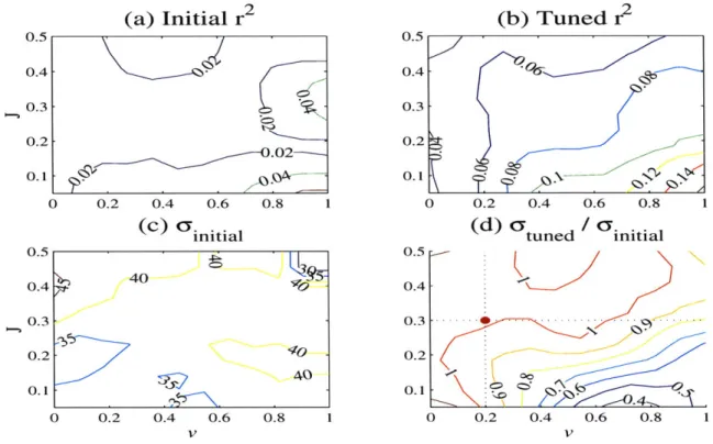
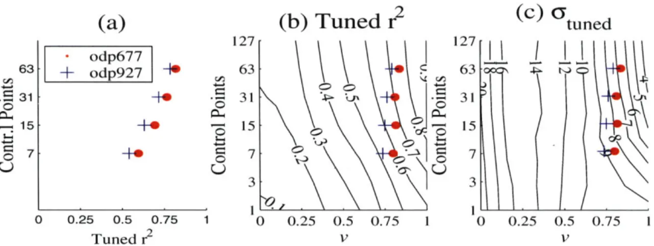
(a) Initial r2 (b) Tuned r2 0.5 0.5 0.4 0.4 0.3 0.3 0.2 0.2 .... 5.... ..- 0 -(c) 0_Yinitial (d) cytuned Cy initial 0.5 _0.5 4O. 0.4 400.4-0.3- 0.3-0.2 00.2 40 0 0.1 0.1 -0 0.2 0.4 0.6 0.8 1 0 0.2 0.4 0.6 0.8 1 V V

Figure 1-7: Orbitally-tuning the Brunhes Matuyama Magnetic Reversal Date. The contour plots are given as: (a) The initial squared cross-correlation between the jit-tered signal, V)(t'), and the target curve, r(t). (b) The tuned squared cross-correlation value. (c) The initial root mean square age-model error, -rms. (d) The ratio of initial to final rms age error, o-(t' + p(t'))rms/o(t')rms . The y-ordinate indicates the degree

of jitter, J, and the x-ordinate gives the percent orbital variance, v. The red dot indicates the best estimate of the orbital variance and jitter typical of ocean sediment core 6180 records.

near zero everywhere and the initial rms age error is on the order of 40KY (ref Fig-ure 1-7a and c). Since only one ACP is permitted, tuning with XCM increases the squared cross-correlation by only 0.04 to 0.1. In regions with J less than 0.3 and v greater than 0.1 the tuning decreased the rms deviation from true age (i.e. an at least partially correct adjustment slope) and the tuning is considered skillful (ref Eq 1.9). In chapter two the degree of jitter for 6180 records is estimated as 0.3 and in chapter three the fraction of 6180 variance linearly related to obliquity and precession is esti-mated as 0.2. This puts the 6180 record just outside the region where tuning shows skill. A 6180 record with either slightly lower J or higher v could well lie within a region of greater skill, and there are indications ODP677 is such a record [see Shack-leton et al, 1990]. The skill of XCM in tuning synthetic signals is thus consistent

(a) Initial r2 0 0.2 0.4 0.6 mC Yiitial (b) Tuned r 0.8 0 0.2 0.4 0.6 0.8 (d) a / C. . tuned initial 0.6 0.8 1 0 0.2 0.4 0.6 0.8 1

Figure 1-8: Same as Figure 1-7, but ACPs are located at 270 and 530KY BP, and the final age is anchored at 800KY BP. The dot indicates the estimated orbital variance and degree of jitter of the 6180 records.

with Johnson's [1982] and Shackleton's [1990] prediction of a more accurate B-M age based on the results of orbital-tuning.

1.4.3

Detailed Age-model Corrections

The second set of examples fixes the start and end times of V)(t') to the true times of 0 and 800KY BP. Two ACPs are introduced at 270 and 530KY BP allowing for three linear segments in approximating p(t'). There are now only half as many data points per ACP, and there is no overall stretching or shrinking of 0(t). Figure 1-8 shows the results of tuning a jittered signal composed of obliquity and red noise to a target signal of obliquity,

$(t') T(t) = 1 -vrW(t') + v6(t') = 9(t) 0.5 0.4 0.3 0.2 0.1 0C 20 15 20 15-0.2 0.4

2 2

(a) Initial r (b) Tuned r

0.5 0.5 0.4 0.4-0.3 0.3-0.2 0.2 .01.002 0.1 0.1 o 0.2 0.4 0.6 0.8 1 0 0.2 0.4 0.6 0.8 1 (C) initial _{(d) tuned} Y initial 0.5 . 0.5-0.4 0.4 20 0.3 0.3 -. 0.2 0.2 ~ 0.1 1f 50.11 0 0.2 0.4 0.6 0.8 1 0 0.2 0.4 0.6 0.8 1 V V

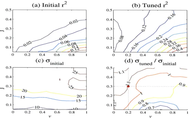
Figure 1-9: Same as Figure 1-8, but the orbital component of the signal, @)(t'), and the target, T(t), is precession.

Figure 1-9 shows a similar tuning result using red noise and precession

$(t') = 1 - vr(t') + \Vp(t')

T(t) = p(t)

The initial orms scales according to J and is equal for both obliquity and pre-cession. The magnitude of the errors is about half the obliquity period while being a full precession cycle. The initial cross-correlation is uniformly small, and for the precession parameter is about half that of obliquity. This accords with higher fre-quencies being more susceptible to the effects of jitter. Tuning increases the obliquity cross-correlation more than precession, and for both scenarios the region of squared cross-correlation greater than 0.18 is coincident with the region where tuning shows skill ('tuned/'initial less than one). Without the benefit of knowing the true age, however, it would be impossible to distinguish where the threshold for an improved age-model lies. For the obliquity simulation, tuning shows some skill with J less than 0.4 and v greater than 0.25, and for precession J less than 0.2 and v greater than

and that approximately 20% of 6180 variance is linearly attributable to obliquity

(vo = 0.13 t 0.07) and precession (v, = 0.1 ± 0.06). This puts the 6180 record out-side the region where tuning shows skill (i.e. orbitally tuning the 6180 records with XCM is expected to make the age-model less accurate). An individual 6180 record with exceptionally low J or high v may be expected to yield a more accurate tuned age-model. Without an independent test for the accuracy of an age-model, however, it is impossible to judge if the tuning was successful.

The original intent of these orbital-tuning exercises was to find an algorithm ca-pable of reliably generating more accurate age-models. A large variety of approaches were attempted, none of which demonstrated greater skill than the examples pre-sented here. Experience with these tuning algorithms indicates that orbital-tuning is capable of correcting for systematic errors over long time scales such as an incorrect date on the B-M boundary. For more detailed corrections to an age-model, primarily

a higher signal-to-noise ratio but also a lower accumulation rate jitter are required than what is estimated for the 6180 record. There are three short-comings of the orbital-tuning approach. (1) There is no statistical test by which the accuracy of an orbitally-tuned record can be judged. (2) Monte Carlo simulations indicate orbital-tuning has poor skill in improving an age-model. (3) Perhaps most importantly, orbital-tuning a priori assumes a model of orbital climate change which it imposes upon the 6180 record. Chapter two develops an alternative age-modeling technique which (1) has objective uncertainty estimates, (2) demonstrates skill in Monte Carlo tests, and (3) is devoid of all orbital assumptions.

Chapter 2

Depth-Tuned Age-models

An age-model based on a single linear age-depth relationship will be stretched or squeezed by each variation in sediment accumulation rate and, subject to certain simplifying assumptions, the variance in linear age from true age is expected to grow at a rate defined by the jitter (J= o2/3, Eq 1.2). A procedure termed depth-tuning

seeks to mitigate the effect of accumulation rate variations by incorporating multiple age-depth relationships into a single age-model. Procedures similar to depth-tuning have been used previously to develop age-models [e.g. Hayes 1976, Williams et al

1988, and Raymo 1997]. Each previous study, however, rejects the age-model implied by mean linear accumulation rates in favor of an orbitally-tuned model. This choice

may reflect the influence of earlier radiometric dates for glacial termination two which accorded with the orbitally tuned age-models [e.g. Broecker et al, 1968; Gallup et al, 1994; and Cheng et al, 1996] and confidence in the Milankovitch theory [e.g. Im-brie et al, 1992]. Recently the Milankovitch theory has come under question [e.g. Winograd et al 1992, Muller and MacDonald 1997, Elkibbi and Rial 2001, and Wun-sch, 2002] and radiometric ages for termination two which conflict with the orbital age-models have been reported [e.g. Esat et al 1999, Henderson and Slowey 2000, and Gallup 2002]. This present study uses significantly more isotopic records than previous studies and corrects for the effects of compaction. The resultant age-model accords with the recent radiometric constraints on termination ages. A statistical model of accumulation rates is developed to provide uncertainty estimates, and a Monte Carlo test with 6180 -like signals indicates the 6180 record can be accurately matched together. Finally, an empirical orthogonal functions (EOF) analysis of ac-cumulation rates demonstrates basin-wide spatial patterns which are themselves of

70o93 60 - ' -0 dsdp552 9 40 ds~p607 - - 30-20 sd 502 0 59 , 10 od.D927 oD-odp 849 o1 677 _{920p 0} 0 od~'924'p md900963 j~ v2e odp 510 04663 O80 odp 46 -10 _v--174 -20 --100 -50 0 50 100 150

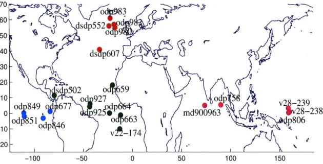
Figure 2-1: The locations of the records used in this study. Shading of dots indicate geographic groupings of cores.

climatic significance.

2.1

The

6180

Records

An ensemble of 26 6180 records from 21 separate drill cores are used for this study whose location are shown in Figure 2-1. The core sites can be divided into four geo-graphical regions; the North Atlantic, Indian Ocean and Western Equatorial Pacific, Equatorial Atlantic, and the Eastern Equatorial Pacific. The geographical distribu-tion heavily favors the Northern Hemisphere and it would be useful to incorporate additional records, particularly in the Southern Hemisphere, as they become avail-able. In five instances two separate 6180 records based on benthic (bottom dwelling) and planktonic (surface dwelling) foraminifera species were measured within the same core. Table 2.1 lists the pertinent statistics and authors of each core. All 6180 records which were available and extend through the Brunhes Matuyama magnetic reversal (B-M) were included in this study. Three of the records are from piston cores

(V28-238, V28-239, and MD900963) while the remainder are Deep Sea Drilling Program (DSDP) or Ocean Drilling Program (ODP) sites which use a composite record spliced

Name Reference Species S At W. Dep Lat Lon DSDP552M DSDP607M ODP980 ODP982 ODP983 ODP677M ODP846M ODP849M ODP851M DSDP502 ODP659M ODP663 ODP664M ODP925 ODP927 v22-174 MD900963M ODP758M ODP806 V28-238M V28-239M

Shackleton and Hall, 1984 Ruddiman et al, 1989 Flower, 1999

Venz et al, 1999 Channell el al, 1997 Shackleton et al, 1990 Mix et al, 1995a Mix et al, 1995b

Ravelo and Shackleton, 1995 Prell, 1982

Tiedemann et al, 1994 de Menocal et al, unpublished Raymo, 1997 Bickert et al, 1997 Cullen et al, 1997 Thierstein et al, 1977 Bassinot et al, 1994 Chen et al, 1995 Berger et al, 1994

Shackleton and Opdyke, 1976 Shackleton and Opdyke, 1976

Table 2.1: A list of the author and characteristics of each core. An 'M' appended to the name of a core indicates the B-M was identified via magnetic susceptibility measurements. From left to right there is 6 80 species B (benthic) and/or P

plank-tonic, the mean sediment accumulation rate (S, cm/KY), the mean interval between 6180 measurements (At, KY), water depth (meters), and the latitude and longitude of each core site.

B B B B,P B B,P B B P P B P B B B,P P P B,P B,P P P 1.9 4.0 12.3 2.5 11.4 3.9 3.7 2.9 2.0 1.9 3.1 3.9 3.7 3.7 4.5 1.8 4.6 1.6 2.0 1.5 0.9 6.4 3.5 1.6 2.3,2.0 .9 2.1,1.8 2.5 3.6 5.0 6.5 3.9 3.0 3.4 2.2 3.2,2.2 5.3 2.3 6.5,6.7 4.8 5.5 5.6 2301 3427 2169 1134 1983 3461 3461 3296 3760 3052 3070 3706 3806 3041 3315 2630 2446 2924 2520 3120 3490 56N 41N 55N 57N 61N IN 3S 0 2S 12N 18N is 0 4N 6N 10s 5N 5N 0 iN 3N 23W 33W 17W 18W 22W 84W 91W 111W 110W 79E 21W 12W 23W 43W 43W 13W 74E 90E 159E 160E 159E Species S

780

11

Age (KY BP)

Figure 2-2: The SPECMAP 6180 stack with the stages and termination mid-points used in this study indicated. The figure is oriented such that upward indicates lighter 3180 (inter-glacial) and the x-axis is arbitrary between stage 19.1 and termination one.

composite depth scale or, if available, the revised composite depth scale was used.

2.2

Building a Depth-Tuned Age-Model

It is useful to define some vocabulary which will be used in developing the depth-tuned age-model. A 6180 event is a feature in the V150 record which can be uniquely identified within each 6180 record. Two types of events are referred to, stages and terminations. Stages are defined as local minima or maxima in the 6180 record [Prell et al, 1986] where the numbering system suggested by Imbrie et al [1984] is used. All the stages referred to in this study have odd numbers after the decimal point, corresponding to low ice volume excursions in the 18O0 record. Terminations are defined as an abrupt shift from glacial to interglacial conditions [Broecker, 1984] where the depth of the midpoint between the local 6180 minima and maxima is used. Figure 2-2 shows the eight termination mid-points and nine stages which are referred to in this study referenced to the SPECMAP 6180 stack [Imbrie et al, 1984].

Depth-tuning is adapted from Shaw's [1964] graphic correlation technique and proceeds in three parts. (1) The Brunhes Matuyama magnetic reversal (B-M) and

termination one are identified in each record and assigned radiometrically estimated ages. Only the portion of the record between the B-M and termination one is retained, between which ages are linearly interpolated with depth. (2) Under the assumption that 6180 variations are global and synchronous, the records are correlated to one another to estimate simultaneous depths between the multiple records. (3) The age estimates (part 1) for the simultaneous depths (part 2) are averaged together to yield a mean age-depth relationship. Assuming variations in accumulation rate are uncorrelated, the mean age estimate is expected to be more accurate than simply taking age as linear with depth in a single core.

Uncertainties inherent in depth-tuning include the ability to uniquely identify and correlate 6180 events given finite sampling resolution and the presence of noise. This possible ambiguity in event identification is addressed by correlating events both visually in section 2.2.2 and objectively in section 2.2.3, and then by a Monte Carlo test in section 2.3. Another uncertainty arises from possible asynchroneity between 6180 events and is addressed in section 2.6.1. Finally, systematic distortions of the age-depth relationships due to changes in mean accumulation rate or core recovery artifacts could bias the resultant age-model, and these issues are also addressed in section 2.6.

2.2.1

Linear Age-Depth Model

To develop a linear age-depth relationship for each 6180 record an age control points

(ACP) is assigned at termination one (10.6 KY BP) and at the B-M magnetic reversal (780 KY BP). The depth of the B-M was reported in the literature as identifiable

via magnetic stratigraphy in 12 of the 21 drill cores, and these cores are indicated by an "M" appended to the name in Table 2.1. For the 6180 records associated with these 12 drill-cores the B-M invariably occurs within 6180 stage 19.1. For core sites at which the B-NI depth was not identifiable, the depth of stage 19.1 is instead used and an age of 780KY BP [see Tauxe et al, 1996] was assigned to both the B-MI and stage 19.1. Between the two ACPs in each record age is linearly interpolated with depth. The resultant linear age-depth relationship is referred to as E(2) where 2 is

the number of ACPs and

j

(d -)-j+, dj, -j (2.1)

tj and d are the age and depth of ACP-1, if and d are the age and depth of

ACP-2, and d. is the depth of each 6180 measurement from each record

j.

2.2.2

Visual Event Correlation

Pisias et al [1984] demonstrated that an ensemble of seven benthic 6180 records could be consistently stratigraphically correlated over the last 300KY in two ways. The first method used visual identification of 6180 events, and under the assumption that events are global and synchronous, correlates the corresponding depths within the ensemble of records. The second method uses Martinson's [1982] correlation algorithm to stretch and squeeze each of the 6180 record to maximize cross-correlation between it and a chosen target 6180 record. This yields a continuous depth transfer function relating each record to the target record. It is shown that both methods produce nearly identical stratigraphic correlations, and it was estimated that benthic 6180 records can be correlated within a resolution of two to four KY. Here both visual event correlation and a cross-correlation maximization routine (XCM) are used to correlate the 26 6180 records between termination one and the B-M. In accordance with Pisias et al's conclusion, both the visual event and XCM correlation methods yield very similar results. Note, however, that Pisias et al sought a 610 stratigraphy and correlated records solely in the depth domain, while depth-tuning seeks an age-model and thus correlates records in the time domain.

The visual event correlation procedure is to (1) put the records onto the E(2

)

J

age-model, (2) identify common isotopic events in each record, (3) average the E2) age of each event over all the records, and (4) constrain each event to occur at the average age for that event.

Seventeen events were visually identified in each core, the midpoint of the eight glacial terminations and stages 5.1, 7.1, 8.5, 11.1, 13.11, 15.1, 17.1, and 19.1. These events are spaced by roughly 50KY with terminations and stages sequentially al-ternating (see Figure 2-2). The end-points are termination one and stage 19.1 or, if available, the B-M magnetic reversal, and are fixed in age by independent radiometric dates. By linearly interpolating age with depth between the end-points, each record