Deep learning methods for the design and understanding of solid materials

Deep Learning Methods for the Design and

Understanding of Solid Materials

by

Tian Xie

Submitted to the Department of Materials Science and Engineering

in partial fulfillment of the requirements for the degree of

Doctor of Philosophy in Materials Science and Engineering

at the

MASSACHUSETTS INSTITUTE OF TECHNOLOGY

September 2020

c

○ Massachusetts Institute of Technology 2020. All rights reserved.

Author . . . .

Department of Materials Science and Engineering

August 7, 2020

Certified by . . . .

Jeffrey Grossman

Professor of Materials Science and Engineering

Thesis Supervisor

Accepted by . . . .

Frances M. Ross

Chair, Departmental Committee on Graduate Studies

Deep Learning Methods for the Design and Understanding

of Solid Materials

by

Tian Xie

Submitted to the Department of Materials Science and Engineering on August 7, 2020, in partial fulfillment of the

requirements for the degree of

Doctor of Philosophy in Materials Science and Engineering

Abstract

The trend of open material data and automation in the past decade offers a unique opportunity for data-driven design of novel materials for various applications as well as fundamental scientific understanding, but it also poses a challenge for conventional machine learning approaches based on structure features. In this thesis, I develop a class of deep learning methods that solve various types of learning problems for solid materials, and demonstrate its application to both accelerate material design and understand scientific knowledge. First, I present a neural network architecture to learn the representations of an arbitrary solid material, which encodes several fundamental symmetries for solid materials as inductive biases. Then, I extend the approach to explore four different learning problems: 1) supervised learning to predict material properties from structures; 2) visualization to understand structure-property relations; 3) unsupervised learning to understand atomic scale dynamics from time series trajectories; 4) active learning to explore an unknown material space. In each learning problem, I demonstrate the performance of the approach compared with previous approaches, and apply it to solve several realistic materials design problems and extract scientific insights from data.

Thesis Supervisor: Jeffrey Grossman

Acknowledgments

I am grateful to many people around me and the wonderful academic environment at MIT. It is fortunate to work on an emerging field with many exciting opportunities to rethink how we do material science. The incredible journey of the last five years would not be possible without the help and support from them.

First and foremost, I would like to thank my advisor professor Jeffrey C. Gross-man. Jeff is a great mentor who has guided and supported me throughout my PhD. He reminds me to think about fundamental breakthroughs rather than incremental improvements, and guides me to shape projects towards broader impact. I am grateful that he is always willing to make time for our discussions despite his busy schedule, and he offers me the freedom to explore new directions. He is also a charismatic leader for our group and creates a group culture that encourages sharing, collaboration, and fun. I am also grateful to him for supporting me to explore future career possibilities and offering advices for career development.

I am grateful to my collaborators who have expanded my knowledge to many different fields of materials science. In particular I would like to thank professor Yang Shao-Horn, professor Jeremiah A. Johnson, professor Adam P. Willard, and professor Rafael Gomez-Bombarelli from the MIT TRI polymer team, as well as current and former students and postdocs including Graham Leverich, Kaitlyn Duelle, Livia Giordano, Shuting Feng, Yivan Jang, Arthur France-Lanord, Yanming Wang, Jeffrey Lopez, Bo Qiao, Michael Stolberg, Megan Hill, Wujie Wang, Sheng Gong. This interdisciplinary team teaches me how to work with researchers from different fields and is extremely beneficial to my professional development. I also thank professor Venkat Viswanathan and Zeeshan Ahmad from Carnegie Mellon University for the collaboration on lithium metal batteries.

I am thankful to my thesis committee members professor Elsa A. Olivetti, pro-fessor Ju Li, and propro-fessor Rafael Gomez-Bombarelli. They provide many valuable advices and suggestions for my projects through committee meetings and individual discussions. I would like add some special thanks to Elsa, who first introduced me to

the field that combines materials science and machine learning in the first year of my PhD. Her passion of using natural language process to extract synthesis route from literature is an important reason why I chose to work on my current field.

It is also important for me to thank all the current and former members of the Grossman group. In particular, I am grateful to Huashan Li who taught me everything about computational material science when I joined the group. I also want to pay special tribute to Arthur France-Lanord and Yanming Wang, who I work closely in the polymer electrolyte project. I also thank Cuiying Jian and Zhengmao Lu for being wonderful officemates, as well as David S Bergsman, Anthony Straub, Brendan Smith, Xining Zang, Thomas Sannicolo, Beza Getachew, Taishan Zhu, Yun Liu, Eric Richard Fadel, Owen Morris, Adam Trebach, Xiang Zhang, Asmita Jana, Cédric Viry, David Chae, Emily Crabb, Ki-Jana Carter, Sheng Gong, Grace Han, and Nicola Ferralis for the time we spent togehter. Additional thanks should be given to Laura M. von Bosau for her passionate administrative support. I have the opportunity to advise several visiting students, William Xu, Pierre-Paul De Breuck, and Doosun Hong, and I thank them for being such awesome students. My graduate life will be much less rewarding and fun without the daily interactions with all the group members. The coffees and football games will always be a special part of my memory at MIT.

Another group of people I would like to thank are the friends who I am fortunate to meet in the last five years. They are Hongzhou Ye, Jiaming Luo, Xinhao Li, Ge Liu, Manxi Wu, Ruizhi Liao, Jiayue Wang, Zhiwei Ding, Yu Xia, Hongzi Mao, Hejin Huang, Yifei Zhang, Danhao Ma, Gufan Yin, Yiqi Ni, Chao Wu, Guo Zong, and many others. The dinners, movies, hiking and many other activities constitute an important part of my life outside campus and will forever be part of memory at MIT. Finally, I would like to thank my parents for their support to my graduate study and career. I feel indebted as my time spent with them is significantly reduced after moving the US. They are always supportive of my decisions, and keep reminding me to relax more and eat healthy. I am grateful for their love and support in the past five years.

Contents

1 Introduction 21

1.1 Motivations for materials science . . . 21

1.1.1 Materials discovery paradigms . . . 21

1.1.2 Application of machine learning in materials . . . 23

1.2 Motivations for deep learning . . . 24

1.2.1 Short introduction to deep learning . . . 24

1.2.2 Inductive biases in neural networks . . . 25

1.3 Unified data representation for solid materials . . . 27

1.3.1 Data representation format . . . 27

1.3.2 Quantum mechanical implications . . . 29

1.3.3 Thermodynamical implications . . . 31

1.4 Problem statement and thesis overview . . . 32

2 Crystal graph convolutional neural networks for the representation learning of solid materials 35 2.1 Introduction . . . 35

2.1.1 Chapter overview . . . 35

2.1.2 Theoretical and practical motivations . . . 36

2.1.3 Related prior research . . . 36

2.2 Invariances in periodic solid materials . . . 36

2.3 Architecture of CGCNN . . . 37

2.3.1 Graph representation of solid materials . . . 37

2.4 Predictive performance . . . 42

2.5 Application to the screening of solid electrolytes for batteries . . . 45

2.5.1 Motivation . . . 45

2.5.2 Stability parameter . . . 47

2.5.3 Predicting the stability parameter with CGCNN ensembles . . 49

2.5.4 Screening of lithium containing compounds for interface stabi-lization . . . 53

3 Visualization of crystal graph convolutional neural networks 59 3.1 Introduction . . . 59

3.1.1 Chapter overview . . . 59

3.1.2 Theoretical and practical motivations . . . 60

3.1.3 Related prior research . . . 60

3.2 Methods . . . 62

3.3 Visualization for different material spaces . . . 64

3.3.1 Overview . . . 64

3.3.2 Perovskite: compositional space . . . 65

3.3.3 Elemental boron: structural space . . . 69

3.3.4 Materials Project: compositional and structural space . . . 75

4 Graph dynamical networks for unsupervised learning of atomic scale dynamics in materials 83 4.1 Introduction . . . 83

4.1.1 Section overview . . . 83

4.1.2 Theoretical and practical motivations . . . 84

4.1.3 Related prior research . . . 85

4.2 Architecture of graph dynamical networks . . . 86

4.2.1 Koopman analysis of atomic scale dynamics. . . 86

4.2.2 Learning feature map function with graph dynamical networks. 87 4.2.3 Hyperparameter optimization and model validation. . . 89

4.4 Application to the understanding of complex dynamics . . . 93

4.4.1 Silicon dynamics in solid-liquid interface . . . 93

4.4.2 Lithium ion dynamics in polymer electrolytes . . . 95

4.4.3 Implications to lithium ion conduction . . . 98

4.5 Discussion . . . 98

4.6 Supplementary notes . . . 101

4.6.1 Computation of global dynamics from local dynamics in the toy system . . . 101

5 Autonomous exploration of the space of polymer electrolytes with Bayesian optimization and coarse-grained molecular dynamics 105 5.1 Introduction . . . 105

5.1.1 Chapter overview . . . 105

5.1.2 Motivations . . . 106

5.2 Coarse Grained Molecular Dynamics-Bayesian Optimization framework 107 5.3 Exploration of the polymer electrolyte space . . . 110

5.3.1 Defining three search spaces . . . 110

5.3.2 Performance of the exploration . . . 111

5.3.3 Understanding the effects of structural modification . . . 112

5.4 Discussion . . . 116

6 Conclusion and outlook 121 6.1 Summary of the thesis . . . 121

List of Figures

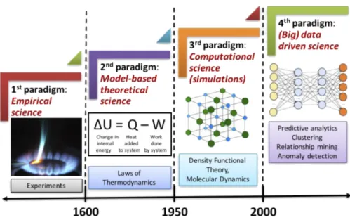
1-1 The four paradigms of science: empirical, theoretical, computational, and data-driven. [3] . . . 22

1-2 Weight sharing in convolution neural network (CNN) and its impact. (a) An illustrative diagram that demonstrates how weights are shared in CNN. [27] (b) The error rate of the best performing models in the ImageNet competition [28]. . . 26

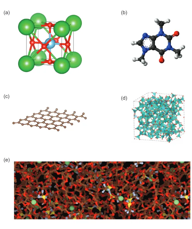
1-3 Representative types of different solid materials. (a) Crystals. Struc-ture of BaTiO3. (b) Molecules. Structure of caffeine. (c) Low

di-mensional materials. Structure of graphene. (d) Amorphous materi-als. Structure of silica glass. [44] (e) Complex materimateri-als. Structure of a mixture of polyethylene oxide (PEO) polymer and lithium bis-(trifluoromethanesulfonyl)-imide (LiTFSI) salts. [45] . . . 30

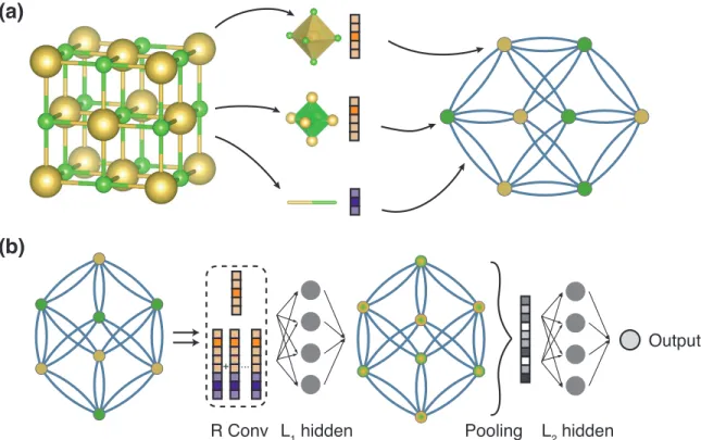
2-1 Illustration of the crystal graph convolutional neural network (CGCNN). (a) Construction of the crystal graph. Crystals are converted to graphs with nodes representing atoms in the unit cell and edges representing atom connections. Nodes and edges are characterized by vectors cor-responding to the atoms and bonds in the crystal, respectively. (b) Structure of the convolutional neural network on top of the crystal graph. 𝑅 convolutional layers and 𝐿1 hidden layers are built on top of

each node, resulting in a new graph with each node representing the local environment of each atom. After pooling, a vector representing the entire crystal is connected to 𝐿2 hidden layers, followed by the

output layer to provide the prediction. . . 38

2-2 The performance of CGCNN on the Materials Project database[70]. (a) Histogram representing the distribution of the number of elements in each crystal. (b) Mean absolute error (MAE) as a function of train-ing crystals for predicttrain-ing formation energy per atom ustrain-ing different convolution functions. The shaded area denotes the MAE of DFT cal-culation compared with experiments[71]. (c) 2D histogram represent-ing the predicted formation per atom against DFT calculated value. (d) Receiver operating characteristic (ROC) curve visualizing the re-sult of metal-semiconductor classification. It plots the proportion of correctly identified metals (true positive rate) against the proportion of wrongly identified semiconductors (false positive rate) under different thresholds. . . 43

2-3 Parity plots comparing the elastic properties: (a) shear modulus 𝐺, and elastic constants (b) 𝐶11, (c) 𝐶12and (d) 𝐶44predicted by the machine

learning models to the DFT calculated values. The shear modulus is predicted using CGCNN and the elastic constants 𝐶11 and 𝐶44 are

predicted using gradient boosting regression while 𝐶12 is predicted

us-ing Kernel ridge regression. The parity plot for shear modulus is on 680 test data points while that for the elastic constants contains all available data (170 points) where each prediction is a cross-validated value. . . 52

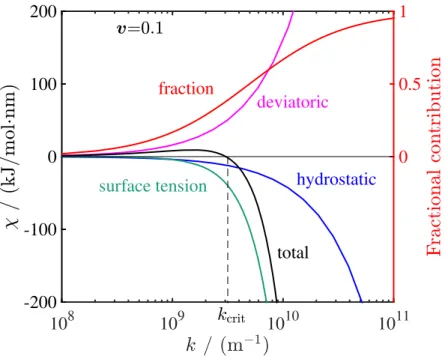
2-4 Contribution of hydrostatic stress, deviatoric stress and surface tension to the stability parameter as a function of surface roughness wavenum-ber. The surface tension term starts dominating at high 𝑘 and ulti-mately stabilizes the interface after 𝑘 = 𝑘crit. The contributions are

plotted for a material with shear modulus ratio 𝐺/𝐺Li = 1 and

Pois-son’s ratio 𝜈 = 0.33 which is not stable (𝜒 > 0) at 𝑘 = 108 _m−1_.

The red line shows the fraction of surface tension contribution to the stability parameter obtained by dividing the absolute value of its con-tribution by the sum of absolute values of all components. . . 54

2-5 Visualization of the latent space representations of 500 random training and 500 random test crystals using t-distributed stochastic neighbor embedding algorithm for CGCNN. . . 55

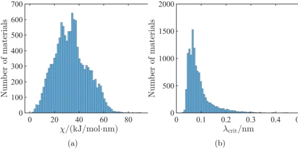
2-6 Results of isotropic screening for 12,950 Li- containing compounds. Distribution of ensemble averaged (a) stability parameter for isotropic Li-solid electrolyte interfaces at 𝑘 = 108 _m−1 _{and (b) critical}

wave-length of surface roughness required for stability. None of the materials in the database can be stabilized without the aid of surface tension. The required critical surface roughness wavenumber depends on the contribution of the stress term in the stability parameter. . . 56

2-7 Isotropic stability diagram showing the position of all solid electrolytes involved in the screening. 𝐺Liis the shear modulus of Li=3.4 GPa. The

critical 𝐺/𝐺Li line separating the stable and unstable regions depends

weakly on the Poisson’s ratio, so the lines corresponding to 𝜈𝑠 = 0.33

and 0.5 are good indicators for assessment of stability. The darker regions indicate more number of materials in the region. . . 58

3-1 The structure of the crystal graph convolutional neural networks. . . 62 3-2 Learning curves for the three representative material spaces. The

mean absolute errors (MAEs) on test data is shown as a function of the number of training data for the perovskites [185, 186], elemental boron [181], and materials project [139] datasets. . . 65 3-3 Visualization of the element representations learned from the perovskite

dataset. (a) The perovskite structure type. (b) Visualization of the two principal dimensions with principal component analysis. (c) Pre-diction performance of several atom properties using a linear model on the element representations. . . 66 3-4 Extraction of site energy of perovskites from total energy above hull.

(a, b) Periodic table with the color of each element representing the mean of the site energy when the element occupies A site (c) or B site (d). . . 68 3-5 Visualization of the local environment representations learned from the

elemental boron dataset. The original 64D vectors are reduced to 2D with the t-distributed stochastic neighbor embedding algorithm. The color of each plot is coded with learned local energy (a), number of neighbors calculated by Pymatgen package [192] (b), and density (c). Representative boron local environments are shown with the center atom colored in red. . . 72 3-6 Example local environments of elemental boron in the four regions:

3-7 The boron fullerene local environments in the boron structural space. The representation of each distinct local environments in the two B40

structures are plotted in the original boron structural space in Fig. 4. 74 3-8 Visualization of the two principal dimensions of the element

repre-sentations learned from the Materials Project dataset using principal component analysis. . . 76 3-9 Visualization of the local oxygen (a) and sulfur (b) coordination

envi-ronments. The points are labelled according to the type of the center atoms in the coordination environments. The colors of the upper parts are coded with learned local energies, and the color of the lower parts are coded with number of neighbors [192], octahedron order parameter, and tetrahedron order parameter [195]. . . 77 3-10 The local energy of oxygen (upper) and sulfur (lower) coordination

environments as a function of atomic number. The blue dotted line denotes the electronegativity of each element. . . 79 3-11 The averaged local energy of 734,077 distinct coordination

environ-ments in the Materials Project dataset. The color is coded with the average of learned local energies while having the corresponding ele-ments as the center atom and the first neighbor atom. White is used when no such coordination environment exists in the dataset. . . 81

4-1 Illustration of the graph dynamical networks architecture. The MD trajectories are represented by a series of graphs dynamically con-structed at each time step. The red nodes denote the target atoms whose dynamics we are interested in, and the blue nodes denote the rest of the atoms. The graphs are input to the same graph convolu-tional neural network to learn an embedding 𝑣_𝑖(𝐾) for each atom that represents its local configuration. The embeddings of the target atoms at 𝑡 and 𝑡 + 𝜏 are merged to compute a VAMP loss that minimizes the errors in Eq. (4.3) [208, 211]. . . 88

4-2 A two-state dynamic model learned for lithium ion in the face-centered cubic lattice. (a) Structure of the FCC lattice and the relative energies of the tetrahedral and octahedral sites. (b-d) Comparison between the local dynamics (left) learned with GDyNet and the global dynamics (right) learned with a standard VAMPnet. (b) Relaxation timescales computed from the Koopman models. (c) Assignment of the two states in the FCC lattice. The color denotes the probability of being in state 0. (d) CK test comparing the long-term dynamics predicted by Koopman models at 𝜏 = 10 ps (blue) and actual dynamics (red). The shaded areas and error bars in (b, d) report the 95% confidence interval from five independent trajectories by dividing the test data equally into chunks. 92

4-3 A four-state dynamical model learned for silicon atoms at solid-liquid interface. (a) Structure of the silicon-gold two-phase system. (b) Cross section of the system, where only silicon atoms are shown and color-coded with the probability of being in each state. (c) The distribution of silicon atoms in each state as a function of z-axis coordinate. (d) Relaxation timescales computed from the Koopman models. (e) Eigen-vectors projected to each state for the three relaxations of Koopman models at 𝜏 = 3 ns. (f) CK test comparing the long-term dynamics predicted by Koopman models at 𝜏 = 3 ns (blue) and actual dynam-ics (red). The shaded areas and error bars in (d, f) report the 95% confidence interval from five sets of Si atoms by randomly dividing the target atoms in the test data. . . 94

4-4 Comparison between the learned states and 𝑞3 order parameters for

silicon atoms at the solid-liquid interface. (a) Cross section of the system, where the silicon atoms are color-coded with their 𝑞3 order

parameters. (b) Distribution of the 𝑞3 order parameter for the silicon

4-5 A four-state dynamical model learned for lithium ion in a PEO/LiTFSI polymer electrolyte. (a) Structure of the PEO/LiTFSI polymer elec-trolyte. (b) Representative configurations of the four Li-ion states learned by the dynamical model. (c) Charge integral of each state around a Li-ion as a function of radius. (d) Relaxation timescales computed from the Koopman models. (e) Eigenvectors projected to each state for the three relaxations of Koopman models at 𝜏 = 0.8 ns. (f) CK test comparing the long-term dynamics predicted by Koopman models at 𝜏 = 0.8 ns (blue) and actual dynamics (red). The shaded areas and error bars in (d, f) report the 95% confidence interval from four independent trajectories in the test data. . . 96

4-6 Contribution from each transition to lithium ion conduction. Each bar denotes the percentage that the transition from state 𝑖 to state

𝑗 contributes to the overall lithium ion conduction. The error bars

report the 95% confidence interval from four independent trajectories in test data. . . 99

4-7 Global relaxation timescales computed for lithium ion hopping in face-centered cubic (FCC) lattice with a 8 dimensional feature space. . . 103

5-1 Illustration of the Coarse Grained Molecular Dynamics-Bayesian Op-timization framework. Schematics of the polymer electrolyte mate-rials design pathway by Bayesian Optimization (BO) guided coarse grained molecular dynamics (CGMD) simulation. Materials design starts with the coarse graining process, to transform the conventional chemical species space to a continuous space composed of CG parame-ters (_{¬→­). This space is then explored by BO guided CGMD} simu-lations in iterations, to predict the resimu-lationships between the transport properties and the associated CG parameters (_{­→®). . . 108}

5-2 Evaluation of the Bayesian Optimization training process. (a) Illustra-tion of the CGMD parameters, which are divided into three groups for describing the properties associated with the anions, secondary sites and backbone chains respectively (from left to right), (b) the inverse of characteristic length scale for each CGMD parameter in the BO training process, (c) the design space exploration efficiency of BO in comparison with random search, and (d) the BO predicted conductiv-ities in comparison with the CGMD test data. . . 110 5-3 Anion effects on lithium conductivity. (a) 3D isosurface plot at the

lithium conductivity value of PEO-LiTFSI, (b) 2D 𝜎_Li+ landscape

projected in 𝜀cat-ani-𝜀cha-ani and 𝑟ani-𝜀cha-ani planes, and (c) 1D cross sectional plots showing the dependence of 𝜎_Li+ on 𝜀cat-ani and

𝑟ani respectively, with the uncertainty evaluations and the acquisition

function values. . . 113 5-4 Effects of secondary sites and polymer backbone chains on lithium

conductivity. A series of 2D 𝜎_Li+ landscape plots for the materials

exploration of (a) secondary sites, and (b) polymer backbone chains. Each subfigure shows the dependence of 𝜎_Li+ on a pair of CGMD

pa-rameters, with the other parameters fixed at the values of the reference PEO-LiTFSI system. The red dots on the graphs denote the reference PEO-LiTFSI system, with the arrows pointing out the directions to maximize 𝜎_Li+. . . 115

5-5 CGMD-BO predictions on conductivity for several common electrolyte systems. The trained BO model predicts conductivities for the PEO-LiTFSI, PEO-LiFSI, PEO-LiPF6 and PEO-LiCl systems, which are

plotted with the uncertainty information (shown as error bars) and their corresponding CG parameters, in comparison with experimental measurements (represented by asterisks)[263, 269, 278, 279]. . . 117

List of Tables

2.1 Properties used in atom feature vector 𝑣(0)_𝑖 . . . 39 2.2 Summary of the prediction performance of seven different properties

on test sets. . . 44 2.3 Comparison of RMSE in log(GPa) for shear and bulk moduli . . . 52 2.4 Solid electrolyte screening results for stable electrodeposition with Li

metal anode together with their materials project id ranked by critical wavelength of surface roughening 𝜆crit required to stabilize

electrode-position. 𝜒 is the stability parameter in kJ/mol·nm which needs to be negative for stability, and 𝑘 = 2𝜋/𝜆 is the surface roughness wavenum-ber. Low 𝑘 corresponds to 𝑘 = 108 _m−1 _{while high 𝑘 corresponds to}

a wavelength 𝜆 = 2𝜋/𝑘 = 1 nm. Only materials with probability of stability 𝑃𝑠 > 0.05 at high 𝑘 are shown. Uncertainty in 𝜒 and 𝜆crit

(standard deviation of their distributions) and 𝑃𝑠 are only shown for

materials whose properties were predicted using CGCNN and not for those whose properties were available in training data. . . 57 3.1 Perovskites with energy above hull lower than 0.2 eV/atom discovered

using combinational search. . . 70 4.1 The charge carried by each state in PEO/LiTFSI. . . 97

Chapter 1

Introduction

1.1

Motivations for materials science

1.1.1

Materials discovery paradigms

The development of new materials plays a central role in the advancement of our civilization. From the stone age to modern society, fundamental innovations in ma-terials have lead to exponential increases of productivity and prosperity. However, the creation and development of a novel material with desired properties is a no-toriously difficult and slow process, mostly due to the lack of understanding of the structure-property relations. Consequently, a significant part of material innovations is still driven by trial-and-error, and many milestone materials are discovered by ac-cident rather than careful design, like copper oxide superconductors in 1986 [1] and perovskite solar cells in 2013 [2].

The paradigms of materials discovery have been gradually shifting from empirical driven towards simulation/data driven over history. 1 Early innovations in materials are usually results from numerous trial-and-errors and empirical knowledge gathered by material scientists. One famous example of this first paradigm is the discovery of a carbonized cotton as the filament of the lightbulb by Thomas Edison in 1880, after

1_{There are multiple different ways to divide the paradigms in materials discovery. Here, we choose}

the narrative by Agrawal et al. in 2016 [3] which divides the entire history into four paradigms. Nevertheless, the overall trend stays the same despite the differences in ways of division.

Figure 1-1: The four paradigms of science: empirical, theoretical, computational, and data-driven. [3]

thousands of failed experiments [4]. Since the early 20th century, the development of quantum mechanics and solid state physics shifted the paradigm to use physical laws and semi-empirical models to guide the design of new materials, as material scientists begin to understand that the atomic structure fundamentally determines material property. Up to today, many material science research are still motivated by exploring neighboring elements in the periodic table, which arranges elements according to periodic trends. In the late 20th century, increasingly powerful computers began to allow the direct computing of material properties by solving the Schrödinger equation, leading to the third paradigm of materials discovery. These simulation methods, called ab-initio simulations, are distinct from earlier physical models as they simulate material properties purely based on first principles like quantum mechanical theory, instead of relying on physical parameters that are fitted using experimental data. The success of ab-initio simulations, especially density functional theory [5], motivated the creation of the Materials Genome Initiative in 2011 [6] to explore the vast space of materials computationally and provide open materials data for the design of novel materials.

paradigm for materials discovery. [3, 7, 8] Since the introduction of Materials Genome Initiative, an increasing number of open databases have emerged that shares both simulation and experiment data of various classes of materials. For example, a recent review paper summarized 10 computational databases and 11 experimental databases that are publicly accessible [7]. There has also been a trend of increased automation in both material synthesis and characterization. [9, 10] The open databases and automation provide an opportunity to develop new data-driven methods that guide the design of novel materials and accelerate the discovery process, and they can also potentially lead to new theories about structure-property relations as patterns emerge from large amounts of data. However, the large size of open material data also indicates that traditional data analysis approaches are incapable of handling these large databases, requiring the development of new machine learning tools for materials. In Chapter 1.1.2, we will overview several classes machine learning tools for solid materials.

1.1.2

Application of machine learning in materials

In this chapter, we overview several types of goals that we aim to achieve by applying machine learning methods to materials discovery. We will focus on their impact to materials design and understanding rather than the methodology, but we list several review papers where various methods are discussed [7, 11, 12]. In chapter 1.4, we will discuss our deep learning approach to provide a unified framework that achieves these different goals.

Property prediction. The goal of property prediction models is to predict material properties based on their structure or chemical composition. Such models can usually run orders of magnitude faster than ab-initio simulations and experiment measurements when they are applied to new materials, thus significantly accelerate material discovery. They been successfully applied to accelerate the screening of organic light-emitting diodes [13], lithium ion batteries [14], etc. A special class of property prediction models are force field models [15], which aim to predict the forces on each atom given the structure of the material. These machine learning force fields

can run close to the speed of classical force fields but have the accuracy close to

ab-initio force fields.

Interpretation and visualization. Material scientists are generally not only interested in discovering new materials, but also understanding how material struc-tures affect their performances. The goal of interpreting machine learning models is to understand the key contributing factors to the property of interest, which can potentially lead to new theory for materials design. Visualization help to understand complex material spaces as they usually include tens of thousands of structures. For example, it can help navigate the complex space of ice structures from zeolite net-works. [16].

Active learning. Active learning aims to explore a complex material space, like intermetallic alloys [17] and the configuration of atomic structures [18], in an iterative fashion that minimizes the number of simulations or experiments. In contrast to property prediction, active learning actively samples the material space and selects materials to evaluate in each iterative step, aiming to thoroughly explore the space with minimum amount of evaluations.

Inverse design. Inverse design aims to directly predict the material structure that has the optimum performance from existing data. Unlike property prediction models that are used to evaluate an existing material space, inverse design aims to predict material structures that are not in the dataset. [19]

1.2

Motivations for deep learning

1.2.1

Short introduction to deep learning

Deep learning is a class of machine learning algorithms that uses multiple layers of neural networks to progressively extract higher level features from the raw input directly from data [20]. In the past ten years, deep learning methods have dramatically improved the state-of-the-art in computer vision, speech recognition, and natural language processing tasks [21], which leads to Hinton, LeCun and Bengio winning

the Turing Award in 2018. Compared with other machine learning methods, deep learning do not rely on human designed features but aims to directly learn the task in an end-to-end fashion. As a result, it usually over-performs other methods when there are large amounts of data, which is a key factor of its success due to the increasing data sizes in multiple fields [22].

The simplest form of neural networks, feedforward networks, include multiple layers of linear transformations plus non-linear activation functions. In each layer, the input vector 𝑥 ∈ R𝑚 _{is transformed by,}

𝑓 (𝑥; 𝑤, 𝑏) = 𝑤|𝑥 + 𝑏, (1.1)

where both 𝑤 ∈ R𝑚×𝑛 _{and 𝑏 ∈ R}𝑛 _{are learned weights. Often non-linearity is added}

via an activation function like ReLU [23] after 𝑓 in each layer. Then, multiple layers of such transformations are applied in a chain, forming multi-layer feedforward networks

𝑓(𝑘)_(𝑓(𝑘−1)_(...𝑓(1)_(𝑥)...)).

A more general neural network differs from this simple form in several aspects: 1) there might be more than one input vectors, 2) each layer might be more com-plicated than linear transformations, and 3) layers might be composed in different ways. However, the general idea is to build complex neural network architecture by combining simple components based on the type of data.

1.2.2

Inductive biases in neural networks

Inductive biases are the set of assumptions in a learning algorithm that are inde-pendent of the observed data. [24] In neural networks, one of the most important inductive biases is the symmetry, or the sharing of weights, within the network ar-chitecture. In the case of feedforward networks, there is no symmetry because the weights are not shared in Eq. 1.1. This means that each individual parameter in the matrix 𝑤 ∈ R𝑚×𝑛 _{has to been learned independently. For a 640 × 480 pixel sized}

image, the input vector size 𝑚 is 640 × 480 = 307, 200, so the number of independent parameters in the first layer will be 307, 200 × 10 = 30, 720, 000 if we choose an output

size 𝑛 of 100, which is almost impossible to learn from data. The lack of sharing of weights in a feedforward neural network makes it unsuitable for complex tasks.

A key breakthrough in modern deep learning is to encode the symmetry of data into the neural network architecture in the form of weight sharing as inductive biases. [25] For example, image data has a translation symmetry for most tasks. To classify an image of a flower, the result should not change if the location of the flower shifts from left to right within the image. This symmetry is not encoded in a feedforward network, which means that a model learned from an image with a flower on the left does not generalize to an image with a flower on the right. The problem is solved by the introduction of convolutional neural network (CNN) [26], which shares the weights across the grid-like structure in images through a convolution operation, as illustrated in Fig. 1-2(a). The weight sharing significantly reduces the number of independent parameters in the networks by incorporating known symmetry in the image data. It has been tremendously successful in many practical applications, and nearly all best performing models in the ImageNet competition are variants of the CNN architecture (Fig. 1-2(b)).

(a) (b)

Figure 1-2: Weight sharing in convolution neural network (CNN) and its impact. (a) An illustrative diagram that demonstrates how weights are shared in CNN. [27] (b) The error rate of the best performing models in the ImageNet competition [28].

Different network architectures are developed to encode the symmetries of various data types into the neural networks. We list several examples below to demonstrate how this concept works in a broader context, and readers can refer to Ref. [25] which discussed the inductive biases in neural networks in depth.

the time invariance in sequential data. [29] RNNs are typically used for language data where sentences and paragraphs are encoded as a sequence of words. Weights are shared across the sequence by applying the same weights to each work sequentially, which enables the generalization to different time in a sequence.

Graph neural networks. Graph neural networks (GNNs) aim to capture the node and edge invariances in graph structured data. [30] It has been used for learning social networks and molecular graphs, as well as many other problems. [31] Weights are shared across both nodes and edges in a graph, which enables the generalization across different graph sizes.

Point networks. Point networks (PointNets) aim to capture the permutation invariance of points in 3D point clouds. [32] Point clouds are a set of data points in 3D space, which are usually generated by 3D scanners. Weights are shared across the points which enable the generalization across 3D space.

1.3

Unified data representation for solid materials

1.3.1

Data representation format

In this section, we seek a general form to represent an arbitrary solid material. We hope this representation will cover various different types of solid materials in a unified way, but still capture the invariances shared by these materials.

We represent the structure of a solid materials as a collection of atoms under a 3D periodic boundary condition. Mathematically, a solid material made up with 𝑁 atoms can be represented by a list of three vectors 𝑚 = {𝑥, 𝑧, 𝑙}, in which

∙ 𝑥 ∈ R𝑁 ×3_{, denoting the coordinates of 𝑁 atoms in 3D space;}

∙ 𝑧 ∈ N𝑁_{, denoting the atomic numbers of each atom in the structure;}

∙ 𝑙 ∈ R3×3_{, denoting the periodic boundary condition of the system, which is}

This representation, which we call periodic solid representation, is widely used to represent solid materials in atomic scale simulations, supported by many existing standard file formats like the Crystallographic Information File (CIF) [33], Protein Data Bank (pdb) file [34], etc. Below, we list several examples of how different types of materials can be represented in this format.

Crystals. Crystal materials (Fig. 1-3(a)) can be naturally represented with pe-riodic solid representation due to their pepe-riodicity. The structure of crystals can measured experimentally using X-ray diffraction (XRD) [35]. Large databases like the Inorganic Crystal Structure Database (ICSD) [36] collects hundreds of thousands of crystal structures.

Molecules. Molecular materials (Fig. 1-3(b)) are often represented by their molecular graphs which describes the connectivity between atoms. However, molec-ular graphs do not capture the 3D structure of molecules, which can be important for many molecular properties. Using the periodic solid representation, molecules can be represented by an isolated molecule with large vacuum space around it un-der a periodic boundary condition. Many molecules have structural polymorphism while forming crystals, which has important pharmaceutical significance. [37] These different structures can be easily capture with periodic solid representation.

Low dimensional materials. Low dimensional materials (Fig. 1-3(c)) are a large class of materials in which periodicity only exists in less than three dimensions. Typical 0D, 1D, and 2D materials includes quantum dots [38], carbon nanotube [39], and graphene [40]. They can be represented with periodic solid representation by introducing large vacuum spaces in dimensions that are not periodic.

Amorphous materials. Amorphous materials (Fig. 1-3(d)) are atomic systems that lack long range order in any direction. [41] Typical amorphous materials include glasses, polymers, gels, etc. Liquids are sometimes considered as amorphous materials as well. Despite the lack of periodicity, representative structures exist for most amor-phous materials. Therefore, they can usually be represented by atomic structures in a very large periodic box where the boundary effects can be ignored.

than one types of above simpler materials. For example, metal-organic frameworks are a class of materials consisting of metal ions coordinated to organic compounds. [42] Solid polymer electrolytes are mixture of polymers and inorganic salts. [43] De-pending on their periodicity, complex materials can also by represented using similar techniques as low dimensional materials and amorphous materials.

1.3.2

Quantum mechanical implications

The periodic solid representation of a material uniquely defines a quantum mechanical system. Given the list 𝑚 = {𝑥, 𝑧, 𝑙}, it defines an atomic system with 𝑁 atoms and 𝑛 electrons under a periodic boundary condition whose full Hamiltonian can be written as, ^ 𝐻 = − 𝑁 ∑︁ 𝐼=1 }2 2𝑀𝐼 ∇2_𝑅𝐼+1 2 ∑︁ 𝐼̸=𝐽 𝑍𝐼𝑍𝐽𝑒2 |𝑅𝐼− 𝑅𝐽| − 𝑁 ∑︁ 𝑖=1 }2 2𝑚∇ 2 𝑟𝑖− 𝑁 ∑︁ 𝐼=1 𝑛 ∑︁ 𝑖=1 𝑍𝐼𝑒2 |𝑅𝐼− 𝑟𝑗| +1 2 ∑︁ 𝑖̸=𝑗 𝑒2 |𝑟𝑖− 𝑟𝑗| (1.2) where 𝑀𝐼, 𝑍𝐼, 𝑅𝐼 are the mass, atomic number, and position of 𝐼th nucleus, 𝑚, 𝑟𝑖

are the mass, and position of 𝑖th electron, 𝑁 and 𝑛 are the total number of nuclei and electrons, } and 𝑒 are Planck’s constant and electron charge.

The many body wavefunction Ψ(𝑟, 𝑅) of this system can be solved with the following eigenvalue problem,

^

𝐻Ψ(𝑟, 𝑅) = 𝐸Ψ(𝑟, 𝑅), (1.3)

which includes both the nuclei and electrons. But in most cases, we can use the Born–Oppenheimer approximation to separate the motion of nuclei and electrons. Assuming that Ψ(𝑟, 𝑅) = Ψ(elec)(𝑟, 𝑅)Ψ(nuc)(𝑅), we could separate the full Hamilto-nian into a nuclei and an electron part,

(a) (b)

(c) _(d)

(e)

Figure 1-3: Representative types of different solid materials. (a) Crystals. Structure of BaTiO3. (b) Molecules. Structure of caffeine. (c) Low dimensional materials.

Structure of graphene. (d) Amorphous materials. Structure of silica glass. [44] (e) Complex materials. Structure of a mixture of polyethylene oxide (PEO) polymer and lithium bis-(trifluoromethanesulfonyl)-imide (LiTFSI) salts. [45]

Then, one could obtain an electronic only eigenvalue problem,

^

𝐻elec(𝑅, 𝑟)Ψ(elec)(𝑟, 𝑅) = 𝐸(𝑅)Ψ(elec)(𝑟, 𝑅). (1.5)

In principle, after obtaining the electronic wavefunction Ψ(elec)_{(𝑟, 𝑅), any material}

property can be computed with its corresponding quantum operators. Note that in this derivation, the periodicity of the system is ignored for simplicity. The derivation under periodic boundary condition is very similar.

Consequently, we know that the periodic solid representation uniquely defines a mapping,

𝑓 : {𝑥, 𝑧, 𝑙} ↦→ 𝑝, (1.6)

where 𝑝 represents an arbitrary material property. This mapping is valid under the Born–Oppenheimer approximation when the motion of the nuclei and electrons can be separated.

We need to pay attention to a special property, energy 𝐸(𝑥, 𝑧, 𝑙), because the system tends to minimize its total energy by changing 𝑥 and 𝑙 and reach a ground state without an external force. It means that the majority of materials in the space of {𝑥, 𝑧, 𝑙} ∈ {R𝑁 ×3_{, N}𝑁_{, R}3×3_{} are not in the ground state and will not form a stable}

material. In most cases, we are interested in stable materials which form a manifold in the space of {R𝑁 ×3_{, N}𝑁_{, R}3×3_}.

1.3.3

Thermodynamical implications

In section 1.3.2, our discussion did not include the temperature effect and is only valid at 0 K. At a finite temperature, the structure of a material will deviate from its ground state structure, forming an ensemble of structures whose distribution is determined by the temperature of the system. It means that macroscopic properties, material properties measured in real life, are determined by this ensemble of structures instead of a single structure. In statistical physics, the structures follow specific distributions according the thermodynamic ensembles. For example, in an isolated system at a fixed

temperature, structures follow a canonical ensemble with a probability distribution,

𝑃 (𝑥, 𝑧, 𝑙) ∝ 𝑒−𝐸(𝑥,𝑧,𝑙)/(𝑘𝐵𝑇 )_{, (1.7)}

where 𝑘𝐵 is the Boltzmann’s constant.

The temperature effect has different implications for different types of materials. For most solid materials, the atoms will only vibrate around its ground-state position at room temperature. It indicates that thermodynamical effect can be approximated with small perturbations to the ground state structure, and Eq. 1.6 still holds if we add the vibration terms into the properties. For liquids and amorphous materials, the energy landscape is more flat, making their macroscopic properties more difficult to define given a single ground state structure.

1.4

Problem statement and thesis overview

In this thesis, we aim to develop a set of unified deep learning methods that solve various learning problems for solid materials. In each chapter of the thesis, we focus on one different learning problem. Each chapter will start by introducing the motiva-tions of the learning problem, then discuss the details of methodology, and end with applications to solve realistic material science problems. The thesis is roughly guided by the following four problems.

Problem 1: how to create a neural network architecture that encodes

material-specific inductive biases and whether such architecture outperforms existing methods?

This problem is the foundation of this thesis. In section 1.3, we defined a unified data representation for the structure of solid materials. This data representation differs from existing data categories like graphs and point clouds, since it has both a discrete component and continuous component. This distinction makes it difficult to use existing neural network architectures for solid materials. In Chapter 2, we will study this problem by introducing a crystal graph convolutional neural networks (CGCNN) architecture [46] that encodes fundamental symmetries of solid materials,

and we will demonstrate the advantages of this architecture over traditional methods and its applications in the design of battery materials [47].

Problem 2: how to extract intuitions that can be understood by human researchers

from the learned representations?

In materials science, it is often desirable to understand the relationship between material structures and properties, since it provides insights that may guide the design of new materials. But improving the interpretability of neural networks has been a challenge for deep learning. In chapter 3, we explore a variety of methods to extract insights from the learned representations, and demonstrate its application to several material systems. [46, 48]

Problem 3: how to learn the representation of atoms in solid materials when no

explicit property labels are available?

In problem 1, we focused on the supervised learning setting that learns the structure-property relations in Eq. 1.6. But it is generally expensive to obtain prop-erty labels either from simulation or experiment. In chapter 4, we explore a dif-ferent scenario to learn the representation of atoms from time-series data without the property labels. The key motivation of this problem is learn a low dimensional representation for atoms and small molecules to understand their complex dynamics behavior from molecular dynamics simulation data. We will also demonstrate the ap-plication of this method to study complex material systems like amorphous polymer electrolytes and liquid-solid interfaces. [45]

Problem 4: how to search an unknown material space in a way that balances

both exploration and exploitation?

The previous problems focus on learning from existing material data. But no data is available when we try to explore an unknown material space. What is the most efficient way to search this space? The major challenge in the problem is the balance of exploration and exploitation. Exploration means searching unknown regions of the space, and exploitation means using existing data to find optimum materials. Designing a strategy to balance these two factors can lead to efficient search of a material space that does not miss potentially important materials. In chapter 5, we

use Bayesian optimization to tackle this problem and apply the approach to the search of polymer electrolytes. [49]

Chapter 2

Crystal graph convolutional neural

networks for the representation

learning of solid materials

2.1

Introduction

2.1.1

Chapter overview

In this chapter, we present a generalized crystal graph convolutional neural networks (CGCNN) framework for the representation learning of periodic solid materials that respects the fundamental invariances. We will first discuss the invariances of periodic solid materials that should be encoded in a neural network architecture. Then, we present how CGCNN encode these invariances into its architecture. Further, we demonstrate the performance of CGCNN in both regression and classification tasks to predict material properties. Finally, we explore the application of CGCNN to a real-world problem for materials design – designing solid electrolytes for lithium metal batteries.

2.1.2

Theoretical and practical motivations

From a theoretical perspective, we aim to solve the supervised learning problem to predict material properties from their structures,

𝑦 = 𝑓 (𝑥, 𝑧, 𝑙), (2.1)

where 𝑓 is a neural network, {𝑥, 𝑧, 𝑙} is a solid material, and 𝑦 is a material property. The goal is to encode the known invariances of solid materials directly into the ar-chitecture of 𝑓 as inductive biases, aiming to achieve better performance than other ML approaches and keep the methods general to various types of solid materials.

From a practical perspective, achieving good performance in the supervised learn-ing problem enables the accelerated screenlearn-ing of new materials in many domains. It is extremely expensive to both measure material properties experimentally or compute them using simulation approaches. A machine learning model that predicts properties with good accuracy can usually run 104_-106 _{orders of magnitude faster than quantum}

mechanical simulations.

2.1.3

Related prior research

The arbitrary size of crystal systems poses a challenge in representing solid materials, as they need to be represented as a fixed length vector in order to be compatible with most ML algorithms. This problem is previously resolved by manually construct-ing fixed-length feature vectors usconstruct-ing simple material properties[50–54] or designconstruct-ing symmetry-invariant transformations of atom coordinates[55–57]. However, the former requires case-by-case design for predicting different properties and the latter makes it hard to interpret the models as a result of the complex transformations.

2.2

Invariances in periodic solid materials

In section 1.3, we proposed an unified representation for solid materials as a three member list 𝑚 = {𝑥, 𝑧, 𝑙}. For a specific solid material, the quantum mechanical

description of the system (Eq. 1.2) guarantees the following invariances.

∙ Permutation invariance. Exchanging two identical atoms (e.g. two hydrogen atoms) will not change the representation of the system. It means that ex-changing 𝑥𝑖 ∈ R3 and 𝑥𝑗 ∈ R3 should not change the learned representation if

𝑧𝑖 = 𝑧𝑗.

∙ Periodicity. Choosing different unit cells for the periodic system will not change the representations of the system. It means that 𝑚1 = {𝑥1, 𝑧1, 𝑙1} and 𝑚2 =

{𝑥2, 𝑧2, 𝑙2} should have the same learned representation if they are different

unit cells of the same periodic structure.

2.3

Architecture of CGCNN

2.3.1

Graph representation of solid materials

The main idea in our approach is to represent the crystal structure by a crystal graph that encodes both atomic information and bonding interactions between atoms, and then build a convolutional neural network on top of the graph to automatically extract representations that are optimum for predicting target properties by training with data. As illustrated in Figure 2-1 (a), a crystal graph 𝒢 is an undirected multigraph which is defined by nodes representing atoms and edges representing connections between atoms in a crystal. The crystal graph is unlike normal graphs since it allows multiple edges between the same pair of end nodes, a characteristic for crystal graphs due to their periodicity, in contrast to molecular graphs. Each node 𝑖 is represented by a feature vector 𝑣𝑖, encoding the property of the atom corresponding to node 𝑖.

Similarly, each edge (𝑖, 𝑗)𝑘 is represented by a feature vector 𝑢(𝑖,𝑗)𝑘 corresponding to

the 𝑘-th bond connecting atom 𝑖 and atom 𝑗.

For the same crystal structure 𝑚 = {𝑥, 𝑧, 𝑙}, there can be multiple different graph representations depending on 1) how connectivity between nodes are determined; 2) how node feature vectors 𝑣(0)_𝑖 are initialized; and 3) how edge feature vectors 𝑢_(𝑖,𝑗)(0)

𝑘

(a)

(b)

R Conv

+ ...

L₁ hidden Pooling L₂ hidden

Output

Figure 2-1: Illustration of the crystal graph convolutional neural network (CGCNN). (a) Construction of the crystal graph. Crystals are converted to graphs with nodes representing atoms in the unit cell and edges representing atom connections. Nodes and edges are characterized by vectors corresponding to the atoms and bonds in the crystal, respectively. (b) Structure of the convolutional neural network on top of the crystal graph. 𝑅 convolutional layers and 𝐿1 hidden layers are built on top of each

node, resulting in a new graph with each node representing the local environment of each atom. After pooling, a vector representing the entire crystal is connected to 𝐿2

In this work, we propose the following methods to construct the graph represen-tations, but other methods are also possible under the framework and several such methods [58] have been proposed since the publication of our work.

Connectivity between nodes. We explore two different methods to deter-mine the connectivity. The first is inspired by Ref. [50] which utilizes the Voronoi tessellation. Only strong bonding interactions are considered in this crystal graph construction. The second method is the nearest neighbor algorithm, where we con-nect 12 nearest neighbors in the initial graph construction. As we will discuss later, the introduction of a convolution function with gated structure (Eq. 2.5) allows the neural networks to automatically learn the importance of each edge. Practically, we find that both methods perform similarly using Eq. 2.5 as the convolution function, significantly outperforming Eq. 2.4.

Node features. The nodes are initialized by a unique mapping from the atomic number to a feature vector 𝑓node : 𝑧𝑖 ↦→ 𝑣

(0)

𝑖 . We designed a feature vector that reflects

the similarity between different elements using their element properties summarized in Table 2.1, which allows the neural networks to generalize to elements that appear less frequently in the dataset.

Table 2.1: Properties used in atom feature vector 𝑣_𝑖(0)

Property Unit Range # of categories Group number – 1,2, ..., 18 18 Period number – 1,2, ..., 91 9 Electronegativity[59, 60] – 0.5–4.0 10

Covalent radius[61] pm 25–250 10 Valence electrons – 1, 2, ..., 12 12 First ionization energy[62](Log) eV 1.3–3.3 10 Electron affinity[63] eV -3–3.7 10

Block – s, p, d, f 4

Atomic volume (Log) cm3_{/mol 1.5–4.3 10}

Edge features. The edges are initialized by a unique mapping from the distance between the connected atoms 𝑓edge : 𝑑𝑖,𝑗 ↦→ 𝑢_(𝑖,𝑗)(0)

𝑘

. In this work, we use the mapping function,

where 𝜇𝑡 = 𝑡 · 0.2 Å for 𝑡 = 0, 1, ..., 𝐾, 𝜎 = 0.2 Å.

2.3.2

Graph neural network architecture

The convolutional neural networks built on top of the crystal graph consists of two ma-jor components: convolutional layers and pooling layers. Similar architectures have been used for computer vision[64], natural language processing[65], molecular finger-printing[66], and general graph-structured data[67, 68] but not for crystal property prediction to the best of our knowledge. The convolutional layers iteratively update the atom feature vector 𝑣𝑖 by “convolution” with surrounding atoms and bonds with

a non-linear graph convolution function.

𝑣_𝑖(𝑡+1)= Conv(︁𝑣_𝑖(𝑡), 𝑣_𝑗(𝑡), 𝑢(𝑖,𝑗)𝑘

)︁

, (𝑖, 𝑗)𝑘∈ 𝒢 (2.3)

The convolution function Eq. 2.3 needs to respect the permutation invariance of atoms, which is achieved by sharing weights between both nodes 𝑣(𝑡)_𝑖 and edges 𝑢(𝑖,𝑗)𝑘.

In this work, we proposed two types of convolution functions. We start with a simple convolution function, 𝑣_𝑖(𝑡+1)= 𝑔 ⎡ ⎣ ⎛ ⎝ ∑︁ 𝑗,𝑘 𝑣(𝑡)_𝑗 ⊕ 𝑢(𝑖,𝑗)𝑘 ⎞ ⎠𝑊_𝑐(𝑡) + 𝑣 (𝑡) 𝑖 𝑊𝑠(𝑡)+ 𝑏(𝑡) ⎤ ⎦ (2.4)

where ⊕ denotes concatenation of atom and bond feature vectors, 𝑊(𝑡)

𝑐 , 𝑊𝑠(𝑡), 𝑏(𝑡) are

the convolution weight matrix, self weight matrix, and bias of the 𝑡-th layer, respec-tively, and 𝑔 is the activation function for introducing non-linear coupling between layers. By optimizing hyperparameters, the lowest mean absolute error (MAE) for the validation set is 0.108 eV/atom. One limitation of Eq. 2.4 is that it uses a shared weight matrix 𝑊(𝑡)

𝑐 for all neighbors of 𝑖, which neglects the differences of interaction

strength between neighbors. To overcome this problem, we design a new convolution function that first concatenates neighbor vectors 𝑧(𝑡)_(𝑖,𝑗)

𝑘 = 𝑣

(𝑡)

𝑖 ⊕ 𝑣

(𝑡)

perform convolution by, 𝑣_𝑖(𝑡+1)= 𝑣(𝑡)_𝑖 +∑︁ 𝑗,𝑘 𝜎(𝑧_(𝑖,𝑗)(𝑡) 𝑘𝑊 (𝑡) 𝑓 + 𝑏 (𝑡) 𝑓 ) ⊙ 𝑔(𝑧 (𝑡) (𝑖,𝑗)𝑘𝑊 (𝑡) 𝑠 + 𝑏(𝑡)𝑠 ) (2.5)

where ⊙ denotes element-wise multiplication and 𝜎 denotes a sigmoid function. In Eq. 2.5, the 𝜎(·) functions as a learned weight matrix to differentiate interactions between neighbors, and adding 𝑣_𝑖(𝑡) makes learning deeper networks easier[69]. We achieve MAE on the validation set of 0.039 eV/atom using the modified convolution function, a significant improvement compared to Eq. 2.4.

After 𝑅 convolutions, the network automatically learns the feature vector 𝑣_𝑖(𝑅)for each atom by iteratively including its surrounding environment. The pooling layer is then used for producing an overall feature vector 𝑣𝑐 for the crystal, which can be

represented by a pooling function,

𝑣𝑐 = Pool

(︁

𝑣(0)₀ , 𝑣₁(0), ..., 𝑣_𝑁(0), ..., 𝑣(𝑅)_𝑁 )︁ (2.6) that satisfies both permutational invariance with respect to atom indexing and pe-riodicity with respect to unit cell choice. In this work, a normalized summation is used as the pooling function for simplicity but other functions can also be used. In addition to the convolutional and pooling layers, two fully-connected hidden layers with the depth of 𝐿1 and 𝐿2 are added to capture the complex mapping between

crystal structure and property. Finally, an output layer is used to connect the 𝐿2

hidden layer to predict the target property ^𝑦.

The training is performed by minimizing the difference between the predicted property ^𝑦 and the DFT calculated property 𝑦, defined by a cost function 𝐽 (𝑦, ^𝑦).

The whole CGCNN can be considered as a function 𝑓 parameterized by weights

𝑊 that maps a crystal 𝒞 to the target property ^𝑦. Using backpropagation and

stochastic gradient descent (SGD), we can solve the following optimization problem by iteratively updating the weights with DFT calculated data,

min

the learned weights can then be used to predict material properties and provide chemical insights for future materials design.

2.4

Predictive performance

To demonstrate the performance of the CGCNN, we train the model using calculated properties from the Materials Project[70]. One key advantage of CGCNN over pre-vious methods is its generality, since our representation cover various types of solid materials (section 1.3). We focus on two types of generality in this work: (1) The structure types and chemical compositions for which our model can be applied, and (2) the number of properties that our model can accurately predict.

The database we used includes a diverse set of inorganic crystals ranging from simple metals to complex minerals. After removing ill-converged crystals, the full database has 46744 materials covering 87 elements, 7 lattice systems and 216 space groups. As shown in Figure 2-2(a), the materials consist of as many as seven different elements, with 90% of them binary, ternary and quaternary compounds. The number of atoms in the primitive cell ranges from 1 to 200, and 90% of crystals have less than 60 atoms(Figure S2). Considering most of the crystals originate from the Inorganic Crystal Structure Database (ICSD)[72], this database is a good representation of known stoichiometric inorganic crystals.

Figure 2-2(b)(c) shows the performance of the two models on 9350 test crystals for predicting the formation energy per atom. We find a systematic decrease of the mean absolute error (MAE) of the predicted values compared with DFT calculated values for both convolution functions as the number of training data is increased. The best MAE’s we achieved with Eq. 2.4 and Eq. 2.5 are 0.136 eV/atom and 0.039 eV/atom, and 90% of the crystals are predicted within 0.3 eV/atom and 0.08 eV/atom errors, respectively. In comparison, Kirklin et al. reports that the MAE of DFT calculation with respect to experimental measurements in the Open Quantum Materials Database (OQMD) is 0.081–0.136 eV/atom depending on whether the energies of the elemental reference states are fitted, although they also find a large MAE of 0.082 eV/atom

0 1 2 3 4 5 6 7 8 9

Number of elements

10

0

10

1

10

2

10

3

10

4

10

5

Co

un

t

10

₁₀

₁₀

₁₀

Number of training crystals

0.0

0.1

0.2

0.3

0.4

0.5

0.6

0.7

0.8

MA

E (

eV

/at

om

)

Eq 4

Eq 5

ROC curve (area = 0.95)

(a)

(b)

(c)

(d)

Figure 2-2: The performance of CGCNN on the Materials Project database[70]. (a) Histogram representing the distribution of the number of elements in each crystal. (b) Mean absolute error (MAE) as a function of training crystals for predicting formation energy per atom using different convolution functions. The shaded area denotes the MAE of DFT calculation compared with experiments[71]. (c) 2D histogram repre-senting the predicted formation per atom against DFT calculated value. (d) Receiver operating characteristic (ROC) curve visualizing the result of metal-semiconductor classification. It plots the proportion of correctly identified metals (true positive rate) against the proportion of wrongly identified semiconductors (false positive rate) under different thresholds.

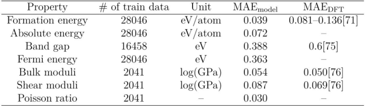
Table 2.2: Summary of the prediction performance of seven different properties on test sets.

Property # of train data Unit MAEmodel MAEDFT

Formation energy 28046 eV/atom 0.039 0.081–0.136[71] Absolute energy 28046 eV/atom 0.072 –

Band gap 16458 eV 0.388 0.6[75]

Fermi energy 28046 eV 0.363 –

Bulk moduli 2041 log(GPa) 0.054 0.050[76] Shear moduli 2041 log(GPa) 0.087 0.069[76]

Poisson ratio 2041 – 0.030 –

between different sources of experimental data. Given the comparison, our CGCNN approach provides a reliable estimation of DFT calculations and can potentially be applied to predict properties calculated by more accurate methods like GW [73] and quantum Monte Carlo[74].

After establishing the generality of CGCNN with respect to the diversity of crys-tals, we next explore its prediction performance for different material properties. We apply the same framework to predict the absolute energy, band gap, Fermi energy, bulk moduli, shear moduli, and Poisson ratio of crystals using DFT calculated data from the Materials Project[70]. The prediction performance of Eq. 2.5 is improved compared to Eq. 2.4 for all six properties (Table S4). We summarize the performance in Table 2.2 and the corresponding 2D histograms in Figure S4. As we can see, the MAE of our model are close to or higher than DFT accuracy relative to experiments for most properties when ∼104 _{training data is used. For elastic properties, the errors}

are higher since less data is available, and the accuracy of DFT relative to experiments can be expected if ∼104 _{training data is available.}

In addition to predicting continuous properties, CGCNN can also predict discrete properties by changing the output layer. By using a softmax activation function for the output layer and a cross entropy cost function, we can predict the classification of metal and semiconductor with the same framework. In Figure 2-2(d), we show the receiver operating characteristic (ROC) curve of the prediction on 9350 test crystals. Excellent prediction performance is achieved with the area under the curve (AUC) at 0.95. By choosing a threshold of 0.5, we get metal prediction accuracy at 0.80,

semiconductor prediction accuracy at 0.95, and overall prediction accuracy at 0.90.

2.5

Application to the screening of solid electrolytes

for batteries

2.5.1

Motivation

In this section, we aim to apply CGCNN to accelerate the discovery of an important type of materials – solid electrolytes for lithium metal batteries. Increased energy densities of Li-ion batteries are crucial for progress towards complete electrification of transportation [77–79]. Among the many possible routes, Li metal anodes have emerged as one of the most likely near-term commercialization options.[80] Coupled with a conventional intercalation cathode, batteries utilizing Li metal anodes could achieve specific energy of > 400 Wh/kg, much higher than the current state of the art ∼250 Wh/kg [81, 82]. Unstable and dendritic electrodeposition on Li metal anode coupled with capacity fade due to consumption of electrolyte has been one of the major hurdles in its commercialization [81, 83–88]. For large scale adoption, a stable, smooth and dendrite-free electrodeposition on Li metal is crucial.

Numerous approaches are being actively pursued for suppressing dendrite growth through the design of novel additives in liquid electrolytes [89–95], surface nanos-tructuring [96, 97], modified charging protocols[98, 99], artificial solid electrolyte interphase or protective coatings [100–102], polymers [103–105] or inorganic solid electrolytes [106–109]. Among these, dramatic improvements in the ionic conductiv-ity of solid electrolytes [110, 111] have made them extremely attractive candidates for enabling Li metal anodes.

A comprehensive and precise criterion for dendrite suppression is still elusive. In-terfacial effects [112, 113] and spatial inhomogeneities within the solid electrolyte like voids, grain boundaries and impurities [114] make the problem challenging. Monroe and Newman performed a dendrite initiation analysis and showed that solid polymer electrolytes with shear modulus roughly twice that of Li could achieve stable