When unstable, growth is less pro poor

HAL Id: halshs-00556672

https://halshs.archives-ouvertes.fr/halshs-00556672

Preprint submitted on 17 Jan 2011

HAL is a multi-disciplinary open access archive for the deposit and dissemination of sci-entific research documents, whether they are pub-lished or not. The documents may come from teaching and research institutions in France or abroad, or from public or private research centers.

L’archive ouverte pluridisciplinaire HAL, est destinée au dépôt et à la diffusion de documents scientifiques de niveau recherche, publiés ou non, émanant des établissements d’enseignement et de recherche français ou étrangers, des laboratoires publics ou privés.

Patrick Guillaumont, Catherine Korachais

To cite this version:

Patrick Guillaumont, Catherine Korachais. When unstable, growth is less pro poor. 2011. �halshs-00556672�

1

Document de travail de la série

Etudes et Documents

E 2008.27

When unstable, growth is less pro poor

Patrick Guillaumont and Catherine Korachais

CERDI

CNRS-Université d'Auvergne

31 p.

2 Summary. – Macroeconomic instability has been increasingly considered as a factor lowering average income growth and by this way is a factor slowing down poverty reduction. But it can also result in slower poverty reduction for a given average rate of growth, due to poverty traps, often examined at the microeconomic level. Testing a model of poverty change on a panel of data for 70 countries from 1981 to 1999, we do find that income instability results in a lower poverty reduction for a given growth. It reflects a distributional effect not fully captured by a change in the Gini coefficient.

Key words – income instability, poverty, inequality, economic growth, growth elasticity of poverty, poverty trap

3 The analysis of the determinants of poverty change across countries considers their impact both through the growth of income per capita and the change in distribution, the latter being generally measured by a Gini coefficient. The impacts of the change in these two variables have been shown to depend on their initial level (Bourguignon, 2003; Heltberg, 2004; Klasen, 2006). It might be a reason why so few cross-section studies have evidenced an impact of macroeconomic factors on poverty change. We argue in this paper that the instability of average income matters. Indeed, macroeconomic instability has been increasingly considered as a factor lowering average income growth and by this way a factor of slower poverty reduction. But it can also be a factor of slower poverty reduction for a given income growth. Here we argue that income volatility slows down poverty reduction because of the existence of poverty traps, often examined at the microeconomic level (for a review see Dercon, 2006). While several micro-studies evidence the impact of shocks and vulnerability on poverty, this relationship is hardly considered at the macroeconomic level. This paper aims to fill in this gap. Using poverty data for 70 countries, we do find that income instability generally results in a lower reduction of poverty for a given growth of income. Figure 1 illustrates the intuition behind the paper.

The paper is organized as follows. The first section describes the ways by which instability may have an impact on poverty at the macro level. The second section develops a model of poverty change taking income instability into account. The third section presents some econometric estimates corresponding to this model. Finally the last section summarizes the results and implications and suggests some further research in that field.

INSY low INSY high -0,50 0,00 0,50 1,00 1,50 2,00 2,50 3,00

Income growth low

Income growth high

S ix y e a r ch a n g e in p o v e rt y

Figure 1. Poverty grows more when income instability is higher.

4

1.

Income instability and poverty change

Many works have examined the effects of income growth on poverty (Ravallion and Chen, 1997; Bourguignon, 2003; Dollar and Kraay, 2002; Adams, 2004; Heltberg, 2004). But only few works deal with the effects of income instability on poverty (see however Guillaumont, 2006, and Guillaumont et al., 2008). The effect of shocks on poverty is yet often considered in the literature, in particular in microeconomic literature, highlighting that negative shocks on income increase the number of people below the poverty line, at least in a short term. Conversely, positive shocks do not result in a proportionate decrease in the extent of poverty (see for example De Janvry and Sadoulet, 2000). For this reason, we are here interested in income instability, i.e. in the succession of positive and negative shocks of income. Instability so defined generally has two types of effects on income: ex ante risk effects, and ex post asymmetry effects due to different responses to falls and rises of income (Guillaumont, 2006). Asymmetry effects are of particular interest with regard to the impact on poverty.

These two effects however are at work through the two channels of transmission by which instability affects poverty, through growth and through income distribution.

(a)

Effect resulting from a lower growth

Poor countries are often characterized by a strong macroeconomic instability. This observation has led to a significant literature on the relation between instabilities and growth (for an overview see Guillaumont, 2006). Several works have evidenced the negative effect of income growth instability on income growth, in general (Ramey and Ramey, 1995; Hnatkovska and Loayza, 2005; Norbin and Yigit, 2005; Aizenmann and Pinto, 2005), and more particularly in Africa (Guillaumont, Guillaumont Jeanneney and Brun, 1999). The negative effects of instability on income growth are generally supposed to come from uncertainty and risk-aversion (ex ante effect). But they can result as well from asymmetric responses to positive and negative shocks (ex post effect).

As income growth is a major factor of poverty reduction, income instability hurts the poor through its negative effect on income growth. Depending on the initial level of income distribution, a lower average income level leads to a higher percentage of population below a “poverty line” (poverty headcount index), and conversely.

In this study, we mainly consider the effects of instability on poverty that do not result from a lower average income1. It means that we do not re-examine per se the relation between instability

1

However, we take this effect into account in the last part in order to estimate the overall effect of income instability on poverty change.

5 and income growth. We then focus on the effects of instability on poverty which are channeled through income distribution.

(b)

Effect resulting from a change in income distribution

If income instability affects income distribution, it affects poverty for a given average income level.

Actually it is reasonable to suppose that for a given income, growth instability affects income distribution and then poverty. This assumption relies on permanent asymmetrical effects of instability on the living conditions of the poor (people below the poverty line) and the “almost poor” (people close to the poverty line). The poor and “almost poor” are particularly exposed to negative shocks and are therefore more vulnerable to the cyclical nature of growth than the rich. Indeed, during downward periods, people who are not insured are pushed under the poverty line while during upward ones they cannot recover enough to return above the line. This corresponds to the underlying idea of the poverty trap.

Referring to microeconomic results (see for example Dercon, 2006), Agénor (2002, 2004) as well as Laursen and Mahajan (2005) and Guillaumont Jeanneney and Kpodar (2005) examine the main reasons as to why the poor are more vulnerable than the non-poor: the poor have little diversified sources of income and they are less qualified and less mobile between sectors and areas. Likewise, they have little access to credit and insurance markets and they depend more on public transfers and social services.

Therefore, during a crisis, the poor and “almost poor” people are the first to suffer from shock induced decisions. For instance, they have problems smoothing their consumption and subsequently their nutritional status (Dercon et al., 2000 for Ethiopia, 1994-95), and parents may remove their children from school (Thomas et al., 2004 for Indonesia, 1998). Furthermore, non qualified workers are the first to be fired (Agénor, 2002) and people may also sell their productive assets (Dercon, 2006), to mention a few. The common point of all these events is that they are asymmetrical: they are not easily reversible once the crisis goes away.

These are the reasons why we suppose that crisis push poor and “almost poor” people into a poverty trap, whereas richer people may be better protected, and as such less vulnerable to instability. It can be analyzed as an asymmetry of the reaction of the different income groups to the fall and rise in income.

Despite the fact that income instability may change the income distribution, only a few cross-country econometric analyses on this subject have been performed (Breen and Garcia-Peñalosa, 2005; Laursen and Mahajan, 2005). The analyses of instability effects among income groups

6 show that the next to last quintile – rather than the last one – appears to be the most affected. We can therefore suppose that the “almost poor” may become “durably poor” under unstable conditions.

This last piece of information leads to the conclusion that income distribution in presence of volatility does not respect the “log normality” distribution assumption as assumed by Bourguignon (2003) and Klasen (2006). It follows that the impact of volatility on income distribution may not be fully captured through the change in the Gini coefficient. Indeed the Gini coefficient is a relevant inequality index, but it is well known that it does not provide any information about the shape of the Lorenz curve. And, as it follows from the previous observations quoted above, a likely result of instability is to change the shape of the Lorenz curve (as illustrated by Figure A.1 in the appendix): as instability affects the poor and almost poor more than the rich people, instability swells the left part of the Lorenz curve.

Subsequently, in order to explain how instability affects poverty reduction due to its effects on income distribution, we need to consider both the effects of income instability channeled by a change in the Gini coefficient as well as the effects channeled by a change in income distribution not reflected by the Gini coefficient.

In summary, macroeconomic instability can increase poverty in two ways: by reducing the average income growth and by making it more unequal. Moreover, such a rising inequality is not necessarily reflected in the change of the Gini coefficient.

2.

A model where poverty change depends on income instability

(a)

Sources of poverty data

Cross country comparisons of poverty changes have been made possible by the work done at the World Bank, and especially by Chen and Ravallion (2004). The data used in that paper are those collected through PovcalNet2. They come from 454 socio-economic sample surveys spanning 97 countries. An assessment is made from these surveys on how aggregate consumption or income is distributed across the population in each country at the date of each survey. Then the proportion of people who do not reach any given “poverty line” is drawn from this distribution.

Since the surveys were not performed in the same years, they give the evolution of poverty over time periods which are neither of the same length nor related to the same years. Indeed, if income instability has an impact on poverty change, this impact is likely to depend on the length of the time period during which it occurs. Poverty data are to be used on identical time periods, which may allow

2

We used PovcalNet data available in 2006. Data available on:

7 interpolation of survey data to non survey years3. That is done by the World Bank’s research group: they use national accounts data and census-based estimates of the population of each country at each date, combine all this information, and calculate the total number of people living below various international poverty lines, as well as other poverty and inequality measures4. Here the poverty line is taken at “one dollar a day” ($1.08 at 1993 international prices).

Three different size samples have been built from these data:

• One is composed by six three year spells of poverty change: 1981-84, 1984-87, 1987-90, 1990-93, 1993-96, and 1996-99. This sample of 70 countries and almost 400 observations allows a panel econometric study. The rather short period legitimates the use of a measure of instability occurring during only three years.

• The second one is composed by three six years spells of poverty change: 1981-87, 1987-93 and 1993-99. This sample of 70 countries and almost 200 observations still allows a panel econometric study, even if it is not optimal. Here we measure the instability occurring during six years, which may have more significant impact.

• The last one is composed by two nine years spells of poverty change: 1981-90 and 1990-99. This sample of 69 countries and 133 observations allows estimating an effect of rather longer term instability.

These three samples enable us to analyze the effect of instability on poverty change on short, on middle and on long term, and then to see the cumulated effect of instability on long term.

(b)

Income instability

The instability of a variable is always relative to a reference value. It is often measured by the standard deviation of the growth rate, i.e. relative to the average growth rate, or preferably by the deviation from a trend. Subsequently the problem lies in the choice of the trend value. Insofar as the series may be neither purely deterministic, nor purely stochastic, the reference value can be estimated from a mixed adjustment, combining at the same time a deterministic element and a stochastic element (method used in various works of the CERDI and chosen by the Committee for Development Policy, United Nations, for the measurement of the instability components of the Economic Vulnerability

3 _{This may lead to underestimate the impact of instability which does not go through the change in the shape of}

the Lorenz curve.

8 Index (UN, 2005, 2008)). The indicator selected here is the average of the quadratic deviation relative to this mixed trend5:

∑

=         ₋ + = n 0 t 2 t t t quadra Yˆ Yˆ Y 1 n 1 100 Ins

Where n = number of years during the period on which instability is calculated

( )

Y and ln

( )

Y aˆ bˆ.ln

(

Y

)

cˆ.t ln exp Yˆ_{t t}  _t = + _{t 1} +      = − ∧ ∧

(c)

Basic factors determining the “income elasticity of poverty”: a parsimonious

model

The incidence of poverty basically depends on the average level of income per capita and on the degree of income inequality. The latter is most often measured by the Gini coefficient. Thus the standard model of poverty change is a function of the respective changes of income per capita and Gini coefficient (Adams, 2004). However, as clearly shown by Bourguignon (2003), the income elasticity of poverty (often named “growth elasticity of poverty”) is arithmetically determined by the initial levels of the income per capita and of the Gini coefficient. It is shown that “both a lesser level of development and a higher level of inequality reduce the growth-elasticity of poverty” (Bourguignon, 2003).

Consequently, for given values of these initial levels there is an expected level of the income elasticity of poverty. This expected elasticity is found to explain to a large extent the poverty change for a given growth of income per capita. Therefore, the model of poverty change must include the initial level of income and the initial Gini coefficient each multiplied both by the growth of income and the change in the Gini coefficient. The model is then the following:

(1) ∆ =α +β ∆ +β ∆ +β ∆ +γ ∆ +γ ∆ +γ₃ ∆ ₀ +ε 0 2 1 0 3 0 2 1 0 .G G G . Y 1 . G G . G G . G . Y Y . Y 1 . Y Y . Y Y . Pov Pov

where Povrepresents the poverty headcount ratio, Pov

Pov ∆

its relative variation,

0

Y the initial income per capita in log,

Y Y ∆

the per capita income growth,

5

In this paper, we calculate income instability from a “global trend” (i.e. estimated using all the available observations from 1960 to 2002). We also use an alternative and calculate it from a “smoothing 12-years trend” (i.e. calculated from the observations of the twelve preceding years).

9 0

G the initial Gini coefficient,

G G ∆

the Gini relative variation.

The reaction of poverty both to income and Gini changes are conditional to initial income (in log) and initial Gini coefficient. The absolute value of the income elasticity of poverty is higher the higher the initial income per capita and the lower the initial Gini coefficient. In the same way, the Gini elasticity of poverty is the higher the higher the initial income per capita and the lower the initial Gini coefficient.

Since a low initial income per capita and a high Gini coefficient are the main factors of a high level of poverty, it is convenient in a more parsimonious model to replace these two variables by one single variable, the initial level of poverty (which then is multiplied by the rate of income growth and by the change in Gini coefficient). It also allows for more degrees of freedom:

(2) ∆ =α₀ +χ₁ ∆ +χ₂ ∆ ₀ +ϕ₁ ∆ +ϕ₂ ∆ .Pov₀ +η G G . G G . Pov . Y Y . Y Y . Pov Pov (2’) ∆ =α +

(

χ +χ

)

∆ +

(

ϕ +ϕ

)

∆ +η G G . Pov . Y Y . Pov . Pov Pov 0 2 1 0 2 1 0

Where is the initial poverty headcount ratio.

It simply means that the level of the per capita income elasticity of poverty depends on the initial level of poverty: its absolute level is expected to be the higher the lower is the initial level of poverty. By the same way the inequality elasticity of poverty is expected to be the higher the lower the initial level of poverty.

(d)

An augmented model of poverty change

The advantage offered by an econometric estimation, compared to the arithmetic calculation of the expected elasticity, is to leave a room for capturing the impact of variables or relationships not adequately reflected in the arithmetic model. We think in particular of possible changes in income distribution not translated into the variation of the Gini coefficient, as well as those resulting from income instability.

Accordingly, in order to identify the effect of instability on poverty, we proceed in three steps. The first one focuses on the “independent effect of instability” (the effect which does not pass through Gini change or income growth). The second step looks at the way instability affects poverty through its overall effect on distribution: therein we take the impact of instability on the Gini coefficient into account. The last step analyses the global effect of instability, taking into account the impact of instability on both Gini coefficient and the growth of income per capita.

10

Residual distributional effect

We identified two ways by which the instability may affect income distribution: one is the change in the Gini coefficient, the other one is a “residual variable” likely to represent the effect of instability on income distribution which is not reflected by a change in the Gini coefficient. Indeed income instability may weaken the assumption of log-normality of the income distribution: poor and “almost poor” people may fall into the poverty trap while rich people might be well insured and stay rich. In this first step, we introduce income instability in our model of poverty in order to assess the effect of instability on poverty, through the latter effect on income distribution. Moreover, it can be expected that this “direct” effect of instability on poverty is itself dependent on the initial level of poverty, as is the reaction of poverty to the change in the Gini coefficient6.

The model to estimate is then the following:

(3) ∆ =α +

(

χ +χ

)

∆ +

(

ϕ +ϕ

)

∆ +

(

λ +λ .Pov

)

.INSY+υ G G . Pov . Y Y . Pov . Pov Pov 0 2 1 0 2 1 0 2 1 0

Where represents income instability during the spell.

Overall distributional effect

Next, we can estimate the total effect of instability on poverty change via its overall effect on income distribution. Following previous findings in the literature, we assume that the change in Gini coefficient is influenced by instability:

(4)       ∆ + δ + δ = ∆ G G net INSY . G G 1 0 Here,       ∆ G G

net is the residual of the equation. It represents the Gini change which does not

result from instability. We then introduce (4) in (3):

(5)

(

)

(

)

(

λ +λ

)

+υ +             ∆ + δ + δ ϕ + ϕ + ∆ χ + χ + α = ∆ INSY . Pov . G G net INSY . . Pov . Y Y . Pov . Pov Pov 0 2 1 1 0 0 2 1 0 2 1 0 6

The higher the initial poverty level, the less the income instability is expected to increase poverty. On the contrary, if the initial poverty level is medium, then there is a more important part of “almost poor” people, and therefore the part of people likely to fall in the poverty trap is greater.

11 That gives the model to estimate:

(6)

(

)

(

)

(

)

(

) (

)

(

λ +ϕ δ + λ +ϕ δ

)

+υ +       ∆ ϕ + ϕ + ∆ χ + χ + δ ϕ + δ ϕ + α = ∆ INSY .. Pov . . . . G G net . Pov . Y Y . Pov . Pov . . . Pov Pov 0 1 2 2 1 1 1 0 2 1 0 2 1 0 0 2 0 1 0 (6’)

₍

₎

₍

₎

+

₍

ψ +ψ

₎

+υ      ∆ ψ + ψ + ∆ ψ + ψ + ψ + ψ = ∆ INSY . Pov . G G net . Pov . Y Y . Pov . Pov . Pov Pov 0 7 6 0 5 4 0 3 2 0 1 0

Note that compared to (3) the coefficient of the Gini change is not modified. But the coefficient of instability is increased since it now captures the total impact of instability and not only that which is channeled through the Gini change.

Total effect including both distributional and growth effect

The final model estimates the global effect of instability on poverty change, considering its impact both on Gini change and on income growth. Remembering the negative effect of instability on income growth, we write:

(7)       ∆ + κ + κ = ∆ Y Y net INSY . Y Y 1 0 Here,       ∆ Y Y

net is the residual of the equation, it also represents the income growth net

effect of instability. We introduce (7) in (6), and the model to estimate is:

(8)

(

) (

)

(

)

(

)

(

) (

)

(

λ +ϕ δ +χ κ + λ +ϕ δ +χ κ

)

+υ +       ∆ ϕ + ϕ +       ∆ χ + χ + κ χ + δ ϕ + κ χ + δ ϕ + α = ∆ INSY .. Pov . . . . . . G G net . Pov . Y Y net . Pov . Pov . . . . . Pov Pov 0 1 2 1 2 2 1 1 1 1 1 0 2 1 0 2 1 0 0 2 0 2 0 1 0 1 0 (8’)

(

)

(

)

+

(

ζ +ζ

)

+υ      ∆ ζ + ζ +       ∆ ζ + ζ + ζ + ζ = ∆ INSY . Pov . G G net . Pov . Y Y net . Pov . Pov . Pov Pov 0 7 6 0 5 4 0 3 2 0 1 0

12

3.

Econometric results

(a)

Descriptive statistics

As mentioned before, the poverty data used are collected from PovcalNet (World Bank). Three samples are built: one with six three years spells, another with three six years spells and the last one with two nine years spells, all between 1981 and 1999. These three panels are not balanced.

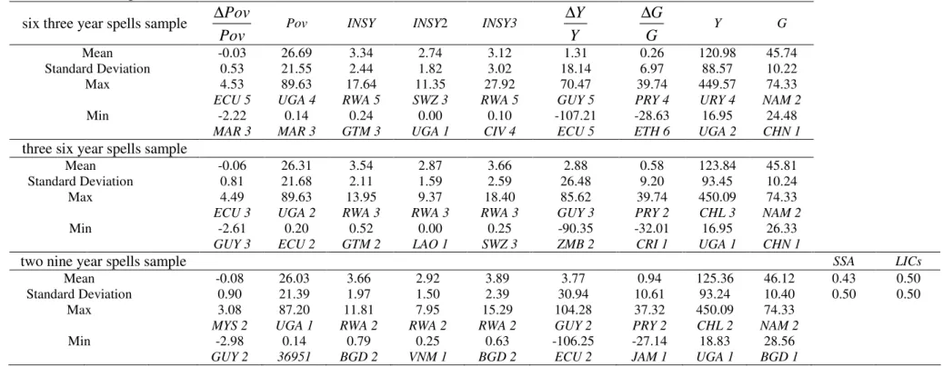
Table B.1 gives the statistical description of the variables in these three panels. Some heterogeneity within these samples can be noted. For instance, looking at the poverty headcount: almost 90% of the population lives with less than one dollar (in PPP) in Uganda whereas the same applies for less than 2% in Morocco or Ecuador (before 1993). It also shows a large heterogeneity in poverty relative change: looking at the six three years spells sample, one can see that the mean of this variable is near 0 (-3%). However, one can observe that the maximum is +453% (Ecuador, 1993-1996) and that the minimum is -222% (Morocco, 1987-1990). Actually, 56% of the observations are positive, 43% are negative which means that poverty increased in 56% of the cases and decreased for only 43% of the observations.

We also observe heterogeneity in levels of income instability. The mean level of INSY is around 3.5% in the three samples, its variance decreases from about 6 in the six three years spells sample to about 4 in the two nine years spells sample. The maximum observed corresponds to the Rwanda genocide and attains there 17% during the period 1993-1996. Table B.2 also gives the list of countries in the two nine years sample, all sorted by their level of income instability.

(b)

Traditional factors of poverty change

This part corresponds to the estimates of the standard model of poverty7 and of a “parsimonious” model which takes Bourguignon (2003) specification into account (model (2)). Table B.3 gives the estimates of these models, with two different estimators (OLS and WITHIN) and with the three different samples. The results are quite similar comparing the estimators. However, different income or Gini elasticities of poverty appear considering the length of the spells.

Results give the main following estimates: • For the standard model:

- Income elasticity of poverty = -2 to -2.5

7

The standard model of poverty is assumed to be :∆ =α +α ∆ +α ∆ +η G G . Y Y . Pov Pov 2 1 0

13 - Gini elasticity of poverty = 2 to 3

• For the “parsimonious augmented” model (model (2), taking into account the initial poverty level of poverty), considering the six year spells sample, which gives the best results, - income elasticity of poverty is -2.9 for an initial poverty level of 10%, and around -1 for an initial

level of 50%.

- Gini elasticity of poverty is 4.2 for an initial poverty level of 10%, and 0.4 for an initial level of 50%.

In summary, income growth and Gini change have a non linear effect on poverty change, which significantly depends on the initial poverty level. In what follows, in order to take this effect into account we refer to the augmented version of the standard model as expressed in model (2).

(c)

The effect of instability on poverty change

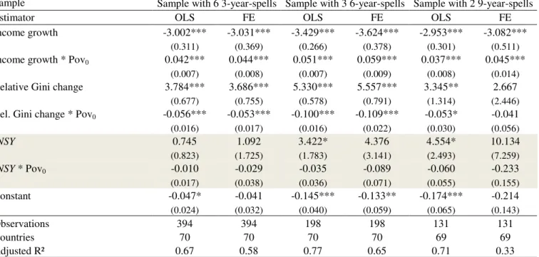
The following estimates (Tables B.4, B.6 and B.7) add as explaining variable the income instability (additively and multiplied by the initial poverty level in order to take the non linear effect of instability on poverty change into account). Coefficients and significances of the standard variables (income growth and Gini change) are not affected by this introduction.

Table B.4 estimates model (3) with the three different samples, and the two estimators (OLS and WITHIN). Table 1 gives the marginal effects of income instability according the different estimates. Income instability is only significant with the samples using six years spells and nine years spells with the OLS estimator. In both of cases, income instability increases poverty change (significant at 10%). To be recalled, in this model the change of the Gini coefficient is a significant control variable, although it is likely to be affected by instability. It captures the impact of all factors affecting poverty through the change in Gini coefficient which includes the likely effects of instability. To assess all the distributional effects of instability, Table B.6 gives estimates of model (6) where the change of the Gini coefficient is introduced net of the effect of income instability8. The coefficient of income instability then represents the effect of income instability on poverty change via its overall effect on inequality. Stronger effects of instability appear: with OLS estimates, income instability has a significant effect on poverty change in the three different samples. Considering the three year spells sample, if income instability increases by one percentage point during a three years period, then poverty change increases by two percentage points over the same period (Table 1). It means for an initial poverty level of 30% (the average of the sample) an increase of poverty level of

8

Table B.5 gives the estimates of the effect on income instability on Gini change. It shows that income instability has a positive and significant effect on Gini change. This is observed with the three samples used. The residuals of these estimates are then introduced in model (6) as “Gini change net of instability”.

14 0.6 percentage points. Both the global results and the effect of instability are stronger when we consider longer periods: if income instability increases by one percentage point during a six years period, then poverty change increases by four percentage points on average over the same period. However, this effect is non linear since the coefficient of the “instability x poverty” multiplicative variable is significant: the effect is all the weaker the initial level of poverty is higher. Table 2 gives the effect of instability on poverty level, on the six year spells sample, for different initial poverty levels and shows that if the initial poverty level is 10%, the overall distributional effect is such that an additional percentage point of instability increases the poverty level by about 0.7 percentage points; if the initial poverty level is 30%, instability makes the poverty level higher by about one percentage point. If it reaches 55%, instability seems to have no distributional effect on poverty. This is easily explainable since we consider the headcount index of poverty (it could be different with the measurement of the poverty gap).

In the nine year periods framework, with the OLS estimates poverty change seems even more affected by an increase of income instability9. It involves that income instability effects on poverty are amplified over time: the effects are even more negative when instability last for a longer time.

Finally, to take into account the total effect of instability, including the effect resulting from a lower growth, Table B.7 estimates model (8): Gini change and income growth variables are both net of the effects of income instability10. Therefore, the coefficient of income instability represents the global effect of income instability on poverty change both through its effect on inequalities and its effect on income. As expected the effect of income instability appears much more important: it is positive and significant in all cases (with all the different spells and estimators). The interactive variable is always negative and significant and as in the previous model, the lower the initial poverty level, the greater the effect of income instability on poverty change.

The effect of income instability is also in this case more important considering longer periods. Best results are obtained when we consider the six year spells and the nine year spells samples.

9

In the nine years periods, a one percentage point increase in income instability generates an increase in the poverty change of about 8.5 percentage points, which means at the average of the sample an increase in the poverty level of 2.3 percentage points.

10

Table B.5 also gives the estimates of the effect on income instability on income growth. It shows that income instability has a negative and significant effect on income growth. This is observed with the three samples used. We use these estimates to calculate “Income growth net of instability” and then to introduce it in model (8).

15 Table 1. Marginal effect of one % point increase of income instability

on the rate of poverty change, for an average poverty level

From OLS estimates

Pure distributional effect of INSY Overall distributional effect of INSY Total effect of INSY

Sample: 6 * 3years none 2.09% 5.12%

Sample: 3 * 6years 3.42% 4.18% 12.41%

Sample: 2 * 9years 4.55% 8.48% 15.70%

From FE estimates

Sample: 6 * 3years none none 4.87%

Sample: 3 * 6years none 3.62% 11.89%

Sample: 2 * 9years none none 15.36%

Calculations made from results from tables B.4, B.6 and B.7, using the average initial poverty level of the sample.

Tips for reading. Example with 2d _{line, 2}d _{column: If INSY increases by one percentage point, the}

Poverty change increases by 4.18 percentage points.

Table 2. Effect of one % point increase of income instability on the poverty level. On the three six years spells sample (in percentage points)

Initial poverty level Estimator Pure distributional effect of INSY Overall distributional effect of INSY Total effect of INSY OLS _{+0.34 +0.68 +1.85} 10% FE +0.00 +0.71 +1.94 OLS _{+1.03 +1.14 +3.45} 30% FE +0.00 +0.93 +3.24 OLS _{+1.71 +0.41 +2.24} 50% FE +0.00 -0.42 +1.11

Calculations made from results from tables B.4, B.6 and B.7.

Another way by which the income growth effect can be roughly compared with the distributional effect of instability is to use a method already by Mo (2001) which although questionable gives an order of magnitude of the relative effects of variables. It consists to measure the respective impact by multiplying the regression coefficients of instability on the intermediate variables (Gini change and income growth) by the regression coefficients of these intermediate variables on poverty. According to our calculates applied on the six year spell sample estimates (Table 3), the distributional effect of instability on poverty change accounts for 33% of the total effect of income instability (of which only 13% corresponding to a change in the Gini coefficient), whereas the ‘income growth’ effect of instability accounts for 67%.

16 Table 3. Relative contributions of the growth effect and the distributional effect of income

instability on poverty change.

Effect of INSY on X Effect of X on Pov.chge Total effect

X beta alpha alpha*

beta Share

…Income growth -4.039 -2.030 8.199 67% 67% Income growth effect of INSY Indirect effect

of INSY through…

…Gini relative change 0.618 2.587 1.599 13%

Direct effect of INSY 2.462 20% 33%

Distributional effect of INSY Total effect of INSY 12.259 100% 100% Total effect of

INSY

All calculations are based on the estimates of equations (3), (4) and (7) made for the three six-year-spells sample (cf. tables B.4 and B.5). They are calculated at the average initial poverty level observed in the sample.

We note that the total effect of instability is clearly non-linear (Table B.7). If we consider the six year spells, the total effect of one percentage point of instability increases the poverty level by about 1.9 percentage points for an initial poverty level of 10%. For an initial level of 30%, instability raises the poverty level by about 3.4 percentage points, and for an initial level of 50%, it raises the poverty level by only 2.2 percentage points.

When the initial poverty level is high the impact of instability on poverty is channeled mainly through lower growth. It can be the result of the headcount definition of poverty adopted.

As robustness checks, Tables B.8 and B.9 give the estimates of models (3), (6) and (8) using different measures of instability: the income instability of Table B.8 is calculated from a 12 years rolling trend (whereas in the main estimates, instability is calculated from a global trend). In Table B.9, instability is measured by the standard deviation of income growth. The given results come from OLS estimates, but the WITHIN estimator gives results that are comparable to Tables B.4, B.6 and B.7. All in all, the results are similar with these two different measures of income instability, no matter which sample is used. Interestingly, the non linear effect of instability leads to a higher poverty whatever the initial level of poverty, although this effect is still decreasing with the initial level.

In addition, in order to consolidate our previous findings, we estimate models (3), (4) and (7) simultaneously with a SUR estimator (Table B.10). Whatever the sample used, the total effect of income instability on poverty change is lower than with the other estimates, since the effect through income growth is divided by two and there is no effect of income instability on the Gini change. However, the distributional effect still accounts for a large share, as we find a similar “direct effect” of income instability compared to previous estimates.

17 To sum up, our hypothesis that income instability contributes to increase poverty by increasing inequalities as well as by lowering income growth is not rejected. Secondly, the distributional effect of instability on poverty is not fully captured by the effect on the Gini coefficient. As it is suggested by these estimates, income instability has a greater distributional incidence on poverty change when the initial poverty level is lower. Indeed, in this case, the part of “almost poor” people is greater than in high poverty countries where more people are already below the poverty line. It follows that income instability has a greater distributional effect on poverty in middle income countries than in low income countries. Table B.11 shows the OLS estimates of models (6) and (8), for the sub-samples LICs and MICs (on the three, six and nine year spells). Indeed, it suggests that the impact of income instability on poverty change is more important in MICs than in LICs. In low income countries, where the initial level of poverty is high, the effect of instability on poverty is probably channeled mainly through a lower growth.

4.

Conclusions, implications for aid effectiveness and further research

We have argued that income instability is likely to affect poverty change beyond its acknowledged effect on income growth. It does so by its effect on income distribution due to the asymmetrical response of poor and almost poor to negative and positive average income shocks.

As almost poor people are more likely to suffer from ups and downs in income than richer ones, income instability may involve stronger inequalities, which is a factor of increasing poverty. Our econometric analysis gives significant results evidencing the relation between income instability and poverty change, reinforcing our previous findings about the effects of income instability on under-five mortality (Guillaumont, Korachais and Subervie, 2008).

Income instability slows down poverty reduction not only because it affects income growth, but because it has a major effect through income distribution and it has such a distribution effect not only by changing the Gini coefficient change: it has also an additional effect on poverty change in the middle and long term not captured by the Gini coefficient. The poverty effect of income instability is then greater when looking at the total income distribution effect.

It has to be kept in mind that instability has a significant impact on the average rate of growth, which is the main determinant of poverty reduction. Our econometric analysis consistently shows the larger global impact of instability on poverty change when taking into account this effect besides those passing through changes in income distribution.

Finally we find that the effect of instability on the change of poverty headcount index is less important in low income countries than in middle income countries. Indeed, the effect of instability on poverty change depends on the initial poverty level, since in low income countries the part of people living below the poverty line (who cannot fall below the line) is higher. On the contrary, middle

18 income countries have a higher part of people above the poverty line and subsequently the probability to observe people falling into the poverty trap is therefore higher. However, income instability may have a negative impact on already poor people and consequently on poverty gap, what remains to be estimated.

The present findings have a major implication for aid effectiveness. In other papers, it has been established that aid is more effective in countries vulnerable to exogenous shocks, because it dampens their negative effect on growth: the stabilizing impact of aid is a main factor of its effectiveness for growth (Guillaumont and Chauvet, 2001; Chauvet and Guillaumont 2004, 2009). According to the argument developed in this paper, if aid has a stabilizing impact on growth, it may lead not only to enhance the average rate of growth, but also to make the growth more pro-poor (see also Guillaumont, 2006). By these two ways it can contribute to poverty reduction, an hypothesis non rejected by preliminary tests not included in this paper.

References

Adams, R. Economic Growth, Inequality and Poverty: Estimating the Growth Elasticity of Poverty. World Development, 32(12), 2004, 1989-2014.

Agénor, P.-R. Business Cycles, Economic Crises, and the Poor testing for Asymmetric Effects. The Journal of Policy Reform, 5(3), 2002, 145-160.

Agénor, P.-R. Macroeconomic Adjustment and the Poor. Journal of Economic Surveys, 18(3), 2004, 351-408.

Aizenmann, J. & B. Pinto. Managing Economic Volatility and Crises: A Practitioner’s Guide, Overview. In J. Aizenmann & B. Pinto (Eds.), Managing Economic Volatility and Crises: A Practitioner’s Guide. The World Bank. Cambridge University Press, 2005.

Bourguignon, F. The Growth Elasticity of Poverty Reduction: Explaining Heterogeneity across Countries and Time Periods. In T. S. Eicher & S. J. Turnovsky (Eds.), Inequality and Growth. The MIT Press, CESifo Seminar Series, 2003, 3-26.

Breen, R. & C. Garcìa-Peñalosa. Income inequality and Macroeconomic Volatility: An Empirical Investigation. Review of Development Economics, 9(3), 2005, 380-398.

Chauvet, L. & P. Guillaumont. Aid, Volatility and Growth Again. Review of Development Economics, forthcoming, August 2009.

Chauvet, L. & P. Guillaumont. Aid and Growth Revisited: Policy, Economic Vulnerability, and Political Instability. In B. Tungodden, N. Stern & I. Kolstad (Eds.), Towards Pro-Poor Policies,

19 Proceedings of the World Bank Annual Conference on Development Economics Europe, 2002. The World Bank. Oxford University Press, 2004, 95-110.

Chen, S. & M. Ravallion. How did the world’s poorest fare since the early 1980s. World Bank Research Observer, 19(2), 2004, 141-169.

De Janvry, A. & E. Sadoulet. Growth, Poverty, and Inequality in Latin America: A Causal Analysis, 1970-94. Review of Income and Wealth, 46(3), 2000, 267-287.

Dercon S. Vulnerability: A Micro Perspective. In F. Bourguignon, B. Pleskovic & J. van der Gaag (Eds.), Securing Development in an Unstable World, Proceedings of the Annual Bank Conference on Development Economics, Amsterdam, 2005. The World Bank, World Bank Publications, 2006, 117-146.

Dercon, S. & P. Krishnan. In Sickness and in Health: Risk Sharing within Households in Rural Ethiopia. Journal of Political Economy, 108(4), 2000, 688-727.

Dollar, D. & A. Kraay. Growth is Good for the Poor. Journal of Economic Growth, 7(3), 2002, 195-225.

Guillaumont, P. (2006). Macro Vulnerability in Low-Income Countries and Aid Responses. In F. Bourguignon, B. Pleskovic & J. van der Gaag (Eds.), Securing Development in an Unstable World, Proceedings of the Annual Bank Conference on Development Economics, Amsterdam, 2005. The World Bank, World Bank Publications, 2006, 65-108.

Guillaumont, P. & L. Chauvet. Aid and Performance: a Reassessment. Journal of Development Studies, 37(6), 2001, 66-92.

Guillaumont, P., S. Guillaumont-Jeanneney & J.F. Brun. How Instability Lowers African Growth. Journal of African Economies, 8(1), 1999, 87-107.

Guillaumont, P., C. Korachais & J. Subervie. How Macroeconomic Instability Lowers Child Survival. UNU-WIDER Research Paper #2008/51, 2008, United Nations University, World Institute for Development Economics Research, Helsinki.

Guillaumont Jeanneney, S. & K. Kpodar. Financial Development, Financial Instability and Poverty. CSAE WPS # 2005-08, 2005, Centre for the Study of African Economies, University of Oxford. Klasen, S. & M. Misselhorn. Determinants of the Growth Semi-Elasticity of Poverty Reduction. Mimeographed, University of Göttingen, Germany, 2006.

Heltberg, R. The Growth Elasticity of Poverty. In A. Shorrocks & R. van der Hoeven (Eds.), Growth, Inequality, and Poverty: Prospects for Pro-Poor Economic Development. United Nations University, World Institute for Development Economics Research, Helsinki. Oxford University Press, 2004, 81-91.

Hnatkovska, V. & N. Loayza. Volatility and Growth. In J. Aizenmann & B. Pinto (Eds.), Managing Economic Volatility and Crises: A Practitioner’s Guide. The World Bank. Cambridge University Press, 2005.

20 Laursen, T. & S. Mahajan. Volatility, Income Distribution, and Poverty. In J. Aizenmann & B. Pinto (Eds.), Managing Economic Volatility and Crises: A Practitioner’s Guide. The World Bank. Cambridge University Press, 2005.

Mo, P. H.. Corruption and Economic Growth. Journal of Comparative Economics, 29, 2001, 66-79. Norrbin, S. C. & F. Pinar Yigit. The Robustness of the Link Between Volatility and Growth of Output. Review of World Economics, 141(2), 2005, 343-356.

Ramey, G. & V. A. Ramey. Cross country evidence on the link between Volatility and Growth. The American Economic Review, 85(5), 1995, 1138-1151.

Ravallion, M. & S. Chen. What Can New Survey Data Tell Us about Recent Changes in Distribution and Poverty? World Bank Economic Review, 11(2), 1997, 357-382.

Thomas, D., K. Beegle, E. Frankenberg, B. Sikoki, J. Strauss & G. Teruel. Education in a crisis. Journal of Development Economics, 74(1), 2004, 53-85.

United Nations. Development Challenges in Sub-Saharan Africa and Post-conflict Countries: Report of the Committee for Development Policy on the Seventh session (14-18 March 2005). United Nations, Department of Economic and Social Affairs. United Nations Publications, 2005.

United Nations. Handbook on the Least Developed Country Category: Inclusion, and Graduation and Special Support Measures. United Nations, Department of Economic and Social Affairs. United Nations Publications, 2008.

21 APPENDIX

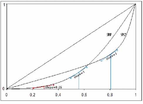
APPENDIX A. FOR A GIVEN GINI COEFFICIENT, INCOME INSTABILITY MAY RESULT IN A MOVE OF THE LORENZ CURVE

Figure A.1. For a given Gini coefficient,

income instability may result in a move of the Lorenz curve.

Let us consider a country, with a given average income per capita and a given Gini coefficient. This country can evidence different income distributions, according to its income instability. Lorenz curves D1 _and D2 _{are two of these possible distributions. We suppose that} D1 _{corresponds to high income} instability, D2 _{to a lower instability.}

Let us imagine that the poverty line is at about 25% of the average income. We can observe from this graph that there’s no “poor” in D2 _{(the slope of the curve is never below 0.25), whereas, in} D1_{, about} 30% of population observes an income which is under the poverty line. Therefore, for a given income per capita and Gini coefficient, we observe different proportions of poverty.

In this paper, we argue that income instability pushes “almost poor” people into a poverty trap. Graphically, income instability makes the income distribution passing from a D2 _{configuration to a} D1 configuration – ceteris paribus.

22 APPENDIX B. EMPIRICAL RESULTS: DESCRIPTIVE STATISTICS AND ECONOMETRIC ANALYSIS

Table B.1. Descriptive statistics

six three year spells sample Pov

Pov

∆

Pov INSY INSY2 INSY3 Y

Y ∆ G G ∆ Y G Mean -0.03 26.69 3.34 2.74 3.12 1.31 0.26 120.98 45.74 Standard Deviation 0.53 21.55 2.44 1.82 3.02 18.14 6.97 88.57 10.22 Max 4.53 89.63 17.64 11.35 27.92 70.47 39.74 449.57 74.33

ECU 5 UGA 4 RWA 5 SWZ 3 RWA 5 GUY 5 PRY 4 URY 4 NAM 2

Min -2.22 0.14 0.24 0.00 0.10 -107.21 -28.63 16.95 24.48

MAR 3 MAR 3 GTM 3 UGA 1 CIV 4 ECU 5 ETH 6 UGA 2 CHN 1

three six year spells sample

Mean -0.06 26.31 3.54 2.87 3.66 2.88 0.58 123.84 45.81

Standard Deviation 0.81 21.68 2.11 1.59 2.59 26.48 9.20 93.45 10.24

Max 4.49 89.63 13.95 9.37 18.40 85.62 39.74 450.09 74.33

ECU 3 UGA 2 RWA 3 RWA 3 RWA 3 GUY 3 PRY 2 CHL 3 NAM 2

Min -2.61 0.20 0.52 0.00 0.25 -90.35 -32.01 16.95 26.33

GUY 3 ECU 2 GTM 2 LAO 1 SWZ 3 ZMB 2 CRI 1 UGA 1 CHN 1

two nine year spells sample SSA LICs

Mean -0.08 26.03 3.66 2.92 3.89 3.77 0.94 125.36 46.12 0.43 0.50

Standard Deviation 0.90 21.39 1.97 1.50 2.39 30.94 10.61 93.24 10.40 0.50 0.50

Max 3.08 87.20 11.81 7.95 15.29 104.28 37.32 450.09 74.33

MYS 2 UGA 1 RWA 2 RWA 2 RWA 2 GUY 2 PRY 2 CHL 2 NAM 2

Min -2.98 0.14 0.79 0.25 0.63 -106.25 -27.14 18.83 28.56

GUY 2 36951 BGD 2 VNM 1 BGD 2 ECU 2 JAM 1 UGA 1 BGD 1

With:

Pov Poverty headcount (% of population)

INSY Income instability, as explained in the text, part 2.2

INSY2 Income instability measured from a 12-years smoothing trend to estimate the reference value

INSY3 Income instability measured as the standard deviation of income growth

Y Average income per capita (at 1993 international prices) G Gini coefficient (comprised between 0 and 100)

SSA Sub Saharan African countries (dummy equal to one if the country is a Sub Saharan African country)

LICs Low Income Countries (dummy equal to one if the country is a Low Income Country)

Pov Pov

∆

Relative poverty change

Y Y

∆

Relative income change (income growth rate)

G G

∆

23 Table B.2. List of countries sorted by decreasing income instability level, in the nine years spells sample

RWA 1990-1999 11.81 LCA 1981-1990 10.42 SWZ 1981-1990 9.58 SLE 1990-1999 8.75 PER 1981-1990 7.88 MOZ 1981-1990 7.37 IRN 1981-1990 7.26 CMR 1981-1990 7.15 MWI 1990-1999 6.75 ETH 1990-1999 6.70 NGA 1981-1990 6.61 PAN 1981-1990 6.25 LCA 1990-1999 6.25 GUY 1981-1990 6.21 ETH 1981-1990 6.04 NER 1981-1990 5.89 MLI 1981-1990 5.86 THA 1990-1999 5.71 CHL 1981-1990 5.51 ZWE 1990-1999 5.44 TTO 1981-1990 5.41 URY 1981-1990 5.41 NIC 1981-1990 5.34 MNG 1990-1999 5.29 MAR 1990-1999 5.16 SLV 1981-1990 4.92 GHA 1981-1990 4.89 CMR 1990-1999 4.86 BDI 1990-1999 4.79 PER 1990-1999 4.75 BRA 1981-1990 4.72 SLE 1981-1990 4.68 JOR 1990-1999 4.68 BDI 1981-1990 4.66 CAF 1981-1990 4.59 PHL 1981-1990 4.54 MYS 1990-1999 4.51 GUY 1990-1999 4.47 VEN 1981-1990 4.39 CRI 1981-1990 4.37 MOZ 1990-1999 4.28 ZMB 1990-1999 4.19 SEN 1981-1990 4.12 PRY 1981-1990 4.10 RWA 1981-1990 4.07 VEN 1990-1999 4.00 MAR 1981-1990 4.00 ZWE 1981-1990 4.00 DOM 1981-1990 3.94 JAM 1981-1990 3.92 NER 1990-1999 3.89 CAF 1990-1999 3.89 ZAF 1981-1990 3.72 MEX 1981-1990 3.66 BWA 1981-1990 3.63 MLI 1990-1999 3.59 CIV 1990-1999 3.59 CHL 1990-1999 3.57 LSO 1990-1999 3.49 NIC 1990-1999 3.48 LSO 1981-1990 3.39 LAO 1981-1990 3.34 IRN 1990-1999 3.32 MDG 1981-1990 3.29 CHN 1981-1990 3.28 GTM 1981-1990 3.26 BFA 1981-1990 3.25 THA 1981-1990 3.24 MRT 1981-1990 3.21 MEX 1990-1999 3.20 ECU 1981-1990 3.15 CIV 1981-1990 3.12 TUN 1981-1990 3.10 BWA 1990-1999 3.05 MYS 1981-1990 3.03 BRA 1990-1999 2.95 CRI 1990-1999 2.91 GMB 1981-1990 2.90 ECU 1990-1999 2.89 MNG 1981-1990 2.86 MWI 1981-1990 2.83 DZA 1990-1999 2.79 CHN 1990-1999 2.76 SWZ 1990-1999 2.74 ZMB 1981-1990 2.72 DZA 1981-1990 2.72 SEN 1990-1999 2.72 TTO 1990-1999 2.70 UGA 1981-1990 2.69 COL 1990-1999 2.67 PAN 1990-1999 2.65 MRT 1990-1999 2.65 SLV 1990-1999 2.64 MDG 1990-1999 2.60 NAM 1990-1999 2.52 HND 1990-1999 2.49 BFA 1990-1999 2.44 HND 1981-1990 2.34 UGA 1990-1999 2.16 PHL 1990-1999 2.16 KEN 1981-1990 2.10 YEM 1990-1999 2.07 EGY 1981-1990 2.01 JAM 1990-1999 1.94 ZAF 1990-1999 1.93 TZA 1990-1999 1.91 NAM 1981-1990 1.90 NGA 1990-1999 1.87 COL 1981-1990 1.86 IND 1990-1999 1.86 TUN 1990-1999 1.84 BOL 1990-1999 1.79 GMB 1990-1999 1.70 PAK 1990-1999 1.69 IND 1981-1990 1.61 PAK 1981-1990 1.61 NPL 1990-1999 1.59 KEN 1990-1999 1.55 TZA 1981-1990 1.44 VNM 1990-1999 1.39 EGY 1990-1999 1.39 BGD 1981-1990 1.34 LKA 1981-1990 1.30 PRY 1990-1999 1.30 KHM 1990-1999 1.23 LKA 1990-1999 1.19 LAO 1990-1999 1.07 GTM 1990-1999 1.04 GHA 1990-1999 1.02 VNM 1981-1990 0.90 BGD 1990-1999 0.79

24 Table B.3. Parsimonious model of poverty change: standard and augmented versions

Sample S a m p l e w i t h 6 3 - y e a r - s p e l l s S a m p l e w i t h 3 6 - y e a r - s p e l l s S a m p l e w i t h 2 9 - y e a r - s p e l l s

Estimator OLS OLS FE FE OLS OLS FE FE OLS OLS FE FE

Income growth -2.087*** -3.001*** -2.120*** -3.051*** -2.316*** -3.410*** -2.467*** -3.658*** -2.181*** -2.958*** -2.510*** -3.195***

(0.231) (0.300) (0.238) (0.330) (0.242) (0.270) (0.273) (0.357) (0.172) (0.282) (0.276) (0.417)

Income growth * Pov0 0.041*** 0.044*** 0.048*** 0.058*** 0.034*** 0.041***

(0.007) (0.008) (0.006) (0.009) (0.007) (0.011)

Relative Gini change 2.368*** 3.754*** 2.354*** 3.663*** 2.844*** 5.183*** 2.981*** 5.460*** 1.994*** 3.186** 1.530 2.490

(0.412) (0.679) (0.428) (0.762) (0.518) (0.582) (0.532) (0.772) (0.630) (1.309) (1.150) (2.279)

Rel. Gini change * Pov0 -0.055*** -0.052*** -0.095*** -0.107*** -0.049 -0.039

(0.016) (0.018) (0.016) (0.021) (0.030) (0.052) Constant -0.010 -0.031** -0.009 -0.032** -0.008 -0.057** -0.004 -0.066** -0.007 -0.061 0.012 -0.062 (0.019) (0.015) (0.020) (0.016) (0.038) (0.027) (0.040) (0.029) (0.047) (0.043) (0.056) (0.053) Observations 401 401 401 401 202 202 202 202 133 133 133 133 Countries 70 70 70 70 70 70 70 70 69 69 69 69 Adjusted R² 0.57 0.68 0.46 0.59 0.63 0.76 0.42 0.65 0.63 0.71 0.25 0.37

Robust standard errors in parentheses. * significant at 10%; ** significant at 5%; *** significant at 1%. Dependent variable: Poverty relative change. Pov0 is the initial poverty headcount.

25 Table B.4. A model of poverty change including income instability

Sample Sample with 6 3-year-spells Sample with 3 6-year-spells Sample with 2 9-year-spells

Estimator OLS FE OLS FE OLS FE

Income growth -3.002*** -3.031*** -3.429*** -3.624*** -2.953*** -3.082***

(0.311) (0.369) (0.266) (0.378) (0.301) (0.511)

Income growth * Pov0 0.042*** 0.044*** 0.051*** 0.059*** 0.037*** 0.045***

(0.007) (0.008) (0.007) (0.009) (0.008) (0.014)

Relative Gini change 3.784*** 3.686*** 5.330*** 5.557*** 3.345** 2.667

(0.677) (0.755) (0.578) (0.791) (1.314) (2.446)

Rel. Gini change * Pov0 -0.056*** -0.053*** -0.100*** -0.109*** -0.053* -0.041

(0.016) (0.017) (0.016) (0.022) (0.030) (0.056) INSY 0.745 1.092 3.422* 4.376 4.554* 10.134 (0.823) (1.725) (1.783) (3.141) (2.493) (7.259) INSY * Pov0 -0.010 -0.029 -0.035 -0.089 -0.060 -0.233 (0.017) (0.038) (0.036) (0.071) (0.055) (0.155) Constant -0.047* -0.041 -0.145*** -0.133** -0.174*** -0.214 (0.024) (0.032) (0.040) (0.059) (0.065) (0.143) Observations 394 394 198 198 131 131 Countries 70 70 70 70 69 69 Adjusted R² 0.67 0.58 0.77 0.65 0.71 0.33

Robust standard errors in parentheses. * significant at 10%; ** significant at 5%; *** significant at 1% Dependent variable: Poverty relative change. Pov0 is the initial poverty headcount.

Random effects estimates have also been done: they give similar results to OLS estimates. In addition, bootstrap shows a stable significance of instability.

Table B.5. Calculations of Gini change and of income change “net of instability effect”

Dependent variable G i n i c h a n g e I n c o m e c h a n g e

Sample 6*3years 3*6years 2*9years 6*3years 3*6years 2*9years INSY 0.329* 0.618* 0.668° -2.109*** -4.039*** -5.857*** (0.169) (0.334) (0.457) (0.468) (0.933) (1.413) Constant -0.000 0.000 0.006 0.074*** 0.145*** 0.223*** (0.007) (0.013) (0.020) (0.017) (0.036) (0.057) Observations 529 264 175 529 264 175 Adjusted R² 0.01 0.02 0.01 0.09 0.13 0.16

OLS estimates. Robust standard errors in parentheses. ° significant at 15%; * significant at 10%; ** significant at 5%; *** significant at 1% Bootstrap shows a stable significance of instability.

26 Table B.6. Effect of instability on the rate of change of poverty via its effect on income distribution

Sample _{Sample with 6 3-years-spells Sample with 3 6-years-spells Sample with 2 9-years-spells}

Estimator OLS FE OLS FE OLS FE

Income growth -3.001*** -3.031*** -3.409*** -3.608*** -2.934*** -3.097***

(0.320) (0.368) (0.272) (0.376) (0.298) (0.535)

Income growth * Pov0 0.042*** 0.045*** 0.050*** 0.057*** 0.036*** 0.046***

(0.008) (0.008) (0.007) (0.009) (0.008) (0.016)

Rel. Gini change net of INSY 3.789*** 3.655*** 5.375*** 5.665*** 3.396** 2.608

(0.675) (0.770) (0.573) (0.823) (1.306) (2.611)

Rel. Gini ch. net of INSY * Pov0 -0.056*** -0.053*** -0.100*** -0.111*** -0.053* -0.039

(0.016) (0.018) (0.016) (0.022) (0.030) (0.061) INSY 2.087° 2.078 8.267*** 9.054** 8.475** 11.207 (1.428) (1.852) (2.711) (3.882) (4.224) (9.047) INSY * Pov0 -0.032 -0.038 -0.149** -0.198** -0.150 -0.237 (0.034) (0.043) (0.064) (0.095) (0.100) (0.209) Pov0 0.000 -0.001 0.002 0.004 0.002 -0.003 (0.001) (0.002) (0.002) (0.005) (0.004) (0.013) Constant -0.052 -0.010 -0.209** -0.245 -0.223 -0.127 (0.063) (0.078) (0.098) (0.164) (0.162) (0.422) Observations 394 394 198 198 131 131 Countries 70 70 70 70 69 69 Adjusted R² 0.67 0.58 0.77 0.65 0.71 0.33

Robust standard errors in parentheses. ° significant at 15% * significant at 10%; ** significant at 5%; *** significant at 1% Dependent variable: Poverty relative change. Pov0 is the initial poverty headcount.

Random effects estimates have also been done: they give similar results to OLS estimates. In addition, bootstrap shows a stable significance of instability.

27 Table B.7. Total effect of income instability on poverty change

Sample _{Sample with 6 3-years-spells Sample with 3 6-years-spells Sample with 2 9-years-spells}

Estimator OLS FE OLS FE OLS FE

Income growth net of INSY -3.001*** -3.031*** -3.409*** -3.608*** -2.934*** -3.097***

(0.320) (0.368) (0.272) (0.376) (0.298) (0.535)

Income growth net of INSY * Pov0 0.042*** 0.045*** 0.050*** 0.057*** 0.036*** 0.046***

(0.008) (0.008) (0.007) (0.009) (0.008) (0.016)

Rel. Gini change net of INSY 3.789*** 3.655*** 5.375*** 5.665*** 3.396** 2.608

(0.675) (0.770) (0.573) (0.823) (1.306) (2.611)

Rel. Gini ch. net of INSY * Pov0 -0.056*** -0.053*** -0.100*** -0.111*** -0.053* -0.039

(0.016) (0.018) (0.016) (0.022) (0.030) (0.061) INSY 8.416*** 8.471*** 22.036*** 23.628*** 25.661*** 29.347*** (1.214) (1.533) (2.948) (4.269) (4.491) (8.635) INSY * Pov0 -0.121*** -0.132*** -0.351*** -0.428*** -0.361*** -0.507** (0.028) (0.036) (0.068) (0.103) (0.101) (0.207) Pov0 0.003*** 0.002 0.010*** 0.012** 0.010** 0.008 (0.001) (0.002) (0.002) (0.005) (0.004) (0.012) Constant -0.275*** -0.236*** -0.703*** -0.768*** -0.878*** -0.819** (0.053) (0.074) (0.098) (0.179) (0.185) (0.403) Observations 394 394 198 198 131 131 Countries 70 70 70 70 69 69 Adjusted R² 0.67 0.58 0.77 0.65 0.71 0.33

Robust st. errors in parentheses. * sig at 10%; ** sig at 5%; *** sig at 1%. Dependent variable: Poverty relative change. Pov0 is the initial poverty headcount.

28 Table B.8. Robustness check of the effect of income instability on poverty change:

instability calculated from a 12 years rolling trend

Sample with 6 3-years-spells Sample with 3 6-years-spells Sample with 2 9-years-spells

Income growth -3.025*** -3.034*** -3.450*** -3.451*** -2.976*** -2.981***

(0.307) (0.304) (0.271) (0.273) (0.303) (0.303)

Income growth net of INSY2 -3.034*** -3.451*** -2.981***

(0.304) (0.273) (0.303)

Income growth * Pov0 0.043*** 0.043*** 0.052*** 0.052*** 0.038*** 0.039***

(0.007) (0.007) (0.007) (0.007) (0.008) (0.008)

Income growth net of INSY 2* Pov0 0.043*** 0.052*** 0.039***

(0.007) (0.007) (0.008)

Relative Gini change 3.730*** 5.312*** 3.367**

(0.681) (0.586) (1.325)

Rel. Gini change net of INSY2 3.680*** 3.680*** 5.311*** 5.311*** 3.354** 3.354**

(0.668) (0.668) (0.579) (0.579) (1.317) (1.317)

Relative Gini change * Pov0 -0.055*** -0.100*** -0.053*

(0.016) (0.016) (0.031)

Rel. Gini ch. net of INSY2 * Pov0 -0.054*** -0.054*** -0.100*** -0.100*** -0.053* -0.053*

(0.016) (0.016) (0.016) (0.016) (0.031) (0.031) INSY2 -0.796 -2.588 2.132 3.701* 2.147 13.379*** 5.522* 7.533* 29.289*** (0.859) (1.750) (1.545) (2.043) (3.052) (3.217) (2.893) (4.318) (4.860) INSY2 * Pov0 0.012 0.071* 0.003 -0.024 0.006 -0.163** -0.053 -0.073 -0.354*** (0.016) (0.042) (0.037) (0.042) (0.075) (0.076) (0.066) (0.102) (0.105) Pov0 -0.003 -0.001 -0.003 0.002 -0.001 0.007* (0.002) (0.002) (0.003) (0.003) (0.003) (0.004) Constant -0.017 0.091 -0.027 -0.147*** 0.026 -0.291*** -0.188*** -0.131 -0.755*** (0.031) (0.074) (0.069) (0.046) (0.106) (0.105) (0.068) (0.142) (0.169) Observations 389 389 389 198 198 198 130 130 130 Countries 70 70 70 70 70 70 69 69 69 Adjusted R² 0.67 0.67 0.67 0.77 0.77 0.77 0.71 0.71 0.71

OLS estimates (FE estimates prove to be almost similar).

Dependent variable: Poverty relative change. Pov0 is the initial poverty headcount.

29 Table B.9. Robustness check of the effect of income instability on poverty change:

instability measured as the standard deviation of income rate of growth

Sample with 6 3-years-spells Sample with 3 6-years-spells Sample with 2 9-years-spells

Income growth -3.015*** -3.018*** -3.447*** -3.428*** -2.975*** -2.946***

(0.308) (0.310) (0.262) (0.264) (0.309) (0.306)

Income growth net of INSY3 -3.018*** -3.428*** -2.946***

(0.310) (0.264) (0.306)

Income growth * Pov0 0.043*** 0.043*** 0.052*** 0.051*** 0.040*** 0.039***

(0.007) (0.007) (0.007) (0.007) (0.008) (0.008)

Income growth net of INSY3 * Pov0 0.043*** 0.051*** 0.039***

(0.007) (0.007) (0.008)

Relative Gini change 3.768*** 5.309*** 3.349**

(0.684) (0.579) (1.311)

Rel. Gini change net of INSY3 3.752*** 3.752*** 5.362*** 5.362*** 3.437*** 3.437***

(0.684) (0.684) (0.582) (0.582) (1.300) (1.300)

Relative Gini change * Pov0 -0.056*** -0.100*** -0.053*

(0.016) (0.016) (0.031)

Rel. Gini ch. net of INSY3 * Pov0 -0.055*** -0.055*** -0.100*** -0.100*** -0.054* -0.054*

(0.016) (0.016) (0.016) (0.016) (0.030) (0.030) INSY3 0.229 0.465 5.377*** 3.322** 8.854*** 18.581*** 3.552 7.425* 20.658*** (0.725) (1.360) (1.253) (1.679) (2.594) (2.824) (2.255) (3.813) (3.835) INSY3 * Pov0 -0.002 -0.001 -0.071** -0.039 -0.174*** -0.318*** -0.050 -0.146 -0.321*** (0.014) (0.032) (0.029) (0.035) (0.063) (0.067) (0.050) (0.092) (0.092) Pov0 -0.001 0.001 0.004 0.009*** 0.003 0.010** (0.002) (0.001) (0.002) (0.002) (0.004) (0.004) Constant -0.035 0.003 -0.142** -0.139*** -0.265*** -0.630*** -0.146** -0.205 -0.729*** (0.023) (0.064) (0.058) (0.039) (0.098) (0.102) (0.057) (0.157) (0.170) Observations 390 390 390 195 195 195 127 127 127 Countries 70 70 70 70 70 70 68 68 68 Adjusted R² 0.67 0.67 0.67 0.77 0.77 0.77 0.71 0.71 0.71

OLS estimates (FE estimates prove to be similar).

Dependent variable: Poverty relative change. Pov0 is the initial poverty headcount.

30

Table B.10. Seemingly Unrelated Regression Estimates

Simultaneous Estimates (1) Simultaneous Estimates (2) Simultaneous Estimates (3)

Sample Six three-year-spells Three six-year-spells Two nine-year-spells

Dependent variable Rel.Pov. Headcount change Rel. Gini change Income growth Rel.Pov. Headcount change Rel. Gini change Income growth Rel.Pov. Headcount change Rel. Gini change Income growth Income growth -3.002*** -3.429*** -2.952*** (0.122) (0.153) (0.199)

Income growth * Pov0 0.042*** 0.051*** 0.037***

(0.004) (0.005) (0.007)

Rel. Gini change 3.784*** 5.330*** 3.345***

(0.341) (0.489) (0.638)

Rel. Gini ch.* Pov0 -0.056*** -0.100*** -0.053**

(0.011) (0.016) (0.021) INSY 0.745 -0.151 -0.972*** 3.422** -0.182 -1.761** 4.554* -0.431 -2.906** (0.836) (0.144) (0.372) (1.636) (0.310) (0.882) (2.622) (0.469) (1.348) INSY * Pov0 -0.010 -0.035 -0.060 (0.018) (0.032) (0.049) Constant -0.047* 0.008 0.046*** -0.145*** 0.012 0.091** -0.174* 0.025 0.144*** (0.026) (0.006) (0.015) (0.055) (0.013) (0.036) (0.093) (0.019) (0.056) Observations 394 198 131