CIRPÉE
Centre interuniversitaire sur le risque, les politiques économiques et l’emploi
Cahier de recherche/Working Paper 06-40
Growth with Equity is Better for the Poor
Sami Bibi
Novembre/November 2006
_______________________
Bibi: Centre Interuniversitaire sur le Risque, les Politiques Économiques et l’Emploi (CIRPÉE) and Poverty and Economic Policy (PEP) Network. Department of Economics, University of Laval, Quebec, Canada G1K 7P4 Fax: +1-418-656-7798
This research was partly funded by the PEP programme of the International Development Research Centre. I am grateful to Jean-Yves Duclos, Abdelkrim Araar, Ali Abdel Gadir Ali, Michael Grimm, Mongi Boughzala, Rim Chatti and Paul Makdissi for useful comments; and to Mathieu Audet, Mohammed Ayadi, Mohammed Goaied, Mohammed Salah Matoussi, Mustapha Kamel Nabli, Rafiq Baccouche, and the Tunisian National Institute of Statistics for kindly providing the micro-data. The usual disclaimer applies.
Abstract:
Putting the combat against poverty to the fore as the main objective of the development process has raised the issue of the linkage between economic growth, inequality and poverty. There is now a growing agreement that booth the rate and the distributional impact of growth are important in fighting poverty. This means that pro-poorness of a given growth rate is more important in certain cases than in others. Using complete and partial poverty orderings, this paper suggests indices of pro-poor growth according to different ethical principals. Evidence from Mexico and Tunisia shows that economic growth periods were to a large extent equitable and even largely pro-poor during the last two decades.
Keywords: Pro-poor growth, Poverty measurement, Robustness analysis JEL Classification: D31, D63, I32, O40
1
Introduction
Enhancing the well-being of the less well-off and reducing inequalities have be-come the principal targets of the development process. The United Nations Gen-eral Assembly in New York notably confirmed these aims in September 2000, when some 189 countries approved, in the context of the Millennium Develop-ment Goals (MDGs), that fighting poverty in all its aspects is the major chal-lenge of the international community. To achieve substantial progress in poverty reduction, most governments and international organisations now agree on both the importance of economic growth and on the need for economic growth to be biased in favor of the poor. Undeniably, absolute poverty is bound to decrease whenever economic growth positively affects the income distribution of the poor. However, it is presumably not the only requirement. Policy makers with an inter-est in poverty reduction are also concerned with the distribution of growth rates amongst the population. This is important because the distribution of any incre-ment to growth will determine the rate at which economic growth is converted into poverty reduction. More precisely, the larger the share of any increment to growth captured by the poor, the higher the pro-poorness feature of economic growth.
The relationship between economic growth and poverty reduction is thus of di-rect relevance to the challenge of fighting poverty in all its aspects. There is grow-ing evidence that achievgrow-ing both high and equitable growth is strengthengrow-ing the linkage between growth and poverty reduction. This represents a major departure from the trickle-down development approach whereby economic growth benefits the more affluent in the first stages of the development process, followed by the less well-off because of the rise in the expenditures of the rich. This means that the development process will be accompanied by a rise in the inequalities since the poor benefit less proportionately from economic growth than do the non-poor. Using data from over 100 countries, Dollar and Kraay (2002) reject the trickle-down approach to poverty reduction. They find that the per capita income of the poorest quintile of the population grew one-for-one with the growth rate of the whole economy over the last four decades; leaving the income distribution unchanged. The principal implications of their findings are that growth is good for poverty reduction, irrespective of the nature of economic growth, and that pro-growth policies are the best poverty reduction strategy. Thus, there is no need for governments to implement specific strategies to achieve the MDGs. They should instead maximise sustainable economic growth by promoting competitive markets and adopting rigorous monetary and fiscal policies.
poverty reduction, they do not offer a significant alternative.1 That growth is good for the poor is self-evident. However, growth is not all that matters. It is under-stood that fighting poverty cannot be continuously relied on redistributive policies in absence of sustainable economic growth. However, there is plenty of evidence suggesting that high rates of growth accompanied with progressive distributional changes will be more effective in reducing poverty than growth patterns that leave the income distribution unchanged.2 Similarly, even if the poor were to benefit from growth as much as the non-poor, the initial distribution of income would still determine the rate of poverty reduction. The higher the level of inequality, the weaker the linkage between poverty reduction and growth; and the higher the growth rate needed to reach a given target of poverty reduction.
That growth is good for the poor is obvious. The real question is how good is economic growth for the poor. Answering this question is the principal ob-jective of this paper. However, computing the extent to which growth is pro-poor is a hotly debated subject.3 For instance, Ravallion and Chen (2003), and Kraay (2004), describe growth as pro-poor whenever it decreases the poverty in-dex of interest. Kakwani and Pernia (2000), Son (2004), and Kakwani and Son (2006), believe that poverty-reducing growth cannot be a sufficient condition for pro-poorness. The growth process should also benefit the poor proportionately more than the non-poor.4 Lopez (2004) and Osmani (2005) find these two def-initions of pro-poorness problematic. They argue that the distributional impact of growth is not all that matters. For instance, Kakwani and Pernia’s (2000) def-inition could conflict with the Pareto principle as an equitable low growth rate can be judged more pro-poor than an inequitable high growth rate even if the for-mer yields less absolute poverty reduction than the latter. Quoting from Osmani (2005),
(...) But if the nature of growth (that is, its distributional impact) is what we are after, why bother to coin a new term (pro-poorness growth)? We already have the concept of equitable growth, which requires growth to be such as to benefit the poor proportionately more
1For Kakwani and Pernia (2000), the findings of Dollar and Kraay (2002) are not robust and in
reality, provide a strong argument for the theory of trickle down development.
2See, for instance, Ravallion (1997, 2004), Bourguignon (2003), Kakwani and Pernia (2000),
White an Anderson (2000), Son (2004), and Kakwani and Son (2006).
3See, among many others, Kakwani and Pernia (2000), Ravallion and Chen (2003), Duclos and
Wodon (2004), Kraay (2004), Son (2004), Osmani (2005), Kakwani and Son (2006), and Araar et al. (2006).
than the rich. Kakwani’s definition does not add anything new to this notion.
Thus, measuring the pro-poorness of growth should include, in addition to the
nature of growth, the scale of poverty reduction in absolute terms enabled by the
growth process. Osmani (2005) goes on to argue that
(...) The quality of pro-poorness is to be attributed not just to the
nature of growth but to the totality of the growth process, including
its rate. Ravallion’s definition refers to the totality of growth process, whereas Kakwani’s stresses the existence of a bias in favor of the poor. We clearly need to combine the strengths of both.
This is precisely the approach followed in this paper. In doing this, the rela-tions between growth, equity, and poverty reduction are addressed in two steps. First, the paper uses complete poverty orderings to develop new measures that capture the extent to which economic growth is pro-poor. Second, it develops the requirements of pro-poor growth using partial poverty orderings. The paper is thus in the spirit of the important contributions of Kakwani and Pernia (2000), Raval-lion and Chen (2003), Kraay (2004), Son (2004), and Kakwani and Son (2006). Methodologically and conceptually, however, the current paper differs from these contributions in a number of important ways:
• This paper makes use of both complete and partial poverty orderings. How-ever, the contributions of Kakwani and Pernia (2000), Kraay (2004), and Kakwani and Son (2006) call only for complete poverty orderings while those of Ravallion and Chen (2003) and Son (2004) are solely based on partial orderings.
• This paper links the concept of pro-poor growth to the desirable proper-ties that poverty measures should satisfy. This enables the characterization of the growth pattern for any ethical order. This makes the methodologi-cal framework general enough to encompass the previous approaches as a special case of the general search for pro-poor growth index.5
• The methodological framework further enables the policy analyst to censor welfare at some upper-bound poverty line so that the ethical focus may be
5For instance, Ravallion and Chen (2003)’s (Son(2004)’s) problem is obtained by checking
first- (second-) order dominance conditions and by setting the upper poverty standard below to infinity.
put (if considered desirable) solely on poverty reduction rather than on a more traditional concept of social welfare improvement.
• To achieve this greater degree of ethical freedom, the ”primal pro-poor growth dominance curves” is relied on more than the dual curves used by Ravallion and Chen (2003) and Son (2004).
In applying the methodology to Mexican and Tunisian data, it is revealed inter
alia that the growth pattern was largely equitable during the two last decades.
These conclusions hold irrespective of the ethical principle chosen to characterize the growth process in these two countries.
The rest of this paper is structured as follows. Section 2 summarizes the theo-retical framework related to the link between economic growth and poverty reduc-tion and suggests a new index that captures the extent to which growth is pro-poor given a pre-selected poverty measure. Section 3 describes how to check for the robustness of pro-poor growth according to different ethical principles. Section 4 computes the extent to which growth was pro-poor in Mexico and Tunisia. Section 5 offers some concluding remarks.
2
Growth contribution to poverty reduction
To assess whether the observed change in the distribution of income is pro-poor, it is conventional to decompose the change in poverty into a change related to a uniform growth of income and a change in relative incomes.6
A more direct approach is to look at growth rates among the poor. For this, let F (y) = p denote the cumulative distribution function (cdf ) of living standards (incomes, for short) giving the proportion of population with income less than y. Inverting the cdf with respect to p gives the quantile function:7
y(p) = F−1(p) for p ∈ [0, 1], (1)
when y(p) is the income level of the individuals whose rank or percentile in the distribution is p. For any given poverty standard z defined in real terms, the pop-ulation can be split into two mutual exclusive groups, namely the poor group and
6See, for instance, Datt and Ravallion (1992) and Kakwani (1997).
7The principal advantage of working with the quantile function is to normalise the population
size to 1. This makes the characterization of the growth pattern in conformity with the principle of
population which states that if an income distribution is replicated several times, overall poverty
the non-poor group. For pro-poorness analysis of economic growth, it is appealing that any index capturing the extent to which growth benefits the poor be indepen-dent of the distribution of growth rates across the non-poor. This is an adapted version of the so-called focus axiom to the context of pro-poor growth analysis.8 Because of this axiom, we make use of the censored income distribution, referred to as y(p; z), instead of the income distribution itself. A censored income dis-tribution sets all income above the poverty cut-off to the poverty standard itself:
y(p; z) = min (y(p), z) . (2)
Further, let x1 be the average of the quantiles x(p), x1(z) be the average of the right censored quantiles x(p; z), x1(p; z) be the average of x(p; z) for the bottom p proportion of the population, xtbe the numerical value of x at date t, and γ(xα,t)
be the growth rate in the pertinent variable xα between the dates t − 1 and t.
To describe how economic growth affects deprivation, we must also address the measurement of poverty. The simplest and most commonly used poverty mea-sure is the headcount ratio, that is the proportion of the population below the poverty line, F (z). When it is deemed to be an appropriate index of poverty, the pro-poorness of economic growth will depend on its ability to bring as many people as possible out of poverty:
γ (yt(Ft(z))) = yt(Ft(z)) − yt−1(Ft(z))
yt−1(Ft(z))
≥ 0. (3)
where, by definition, yt(Ft(z)) = z, yt−1(Ft(z)) is the income of those whose
rank or percentile in the distribution is Ft(z) at date t − 1.
This headcount-decreasing growth could be advantageous, as it is easily un-derstood. Further, for ex-ante analysis, it could be a powerful tool to determine which growth rate is needed to reach a certain target of poverty reduction.9 Nev-ertheless, for an ex-post analysis of poverty-reducing growth, the headcount ra-tio hides the variability of the effects of growth across the poor. As equara-tion (3)
8According to this axiom, any increment to a non-poor person should not matter in measuring
the pro-poorness of economic growth. As argued by Zheng (1997), the desirability of this axiom depends on the perception of the poverty issue. For instance, if poverty is perceived as a relative deprivation, so that the poverty line is fixed as a proportion of the mean income say, this axiom become inappropriate. See Duclos and Wodon (2004) for the use of relative deprivation to study the pro-poorness of distributional changes.
9For instance, in the context of the MDGs, halving the proportion of extreme poverty between
1990 and 2015 is one of the targets of the international community. Using (3), the minimum annual growth rate which is required to reach this goal could be easily inferred.
clearly illustrates, the headcount ratio only records those growth rates that lift peo-ple out of poverty. In other words, only poverty-eliminating growth rates matter, rather than any alleviating growth rates, an example of r-type poverty-reducing growth in Bourguignon and Fields (1997) terminology. Consequently, the effectiveness of economic growth cannot be accurately captured when a large number of the poor benefit from poverty-alleviating growth rates without escaping poverty.10
If in line with Sen (1976), we admit that the poverty measure should be sensi-tive to the welfare change of the poor, a synthetic indicator of poverty-alleviating growth rates could be given by the growth rate in the mean of the censored in-comes γ (y1,t(z)) = R1 0 yt(p; z)dp R1 0 yt−1(p; z)dp − 1 ≥ 0. (4)
Clearly, however, the growth rate in y1,t(z) cannot be a sufficient condition for pro-poorness. An important reason for this is that the income distribution within the poor is far from being equitable. Sen’s (1976) path-breaking study has explained why such inequalities are important in measuring poverty. Logically, they are also important in assessing the pro-poorness of economic growth. Thus, a better pattern of growth satisfies all of Sen’s (1976) core axioms for measur-ing poverty, namely the focus axiom, the monotonicity axiom and the transfer axiom.11
Two approaches have been used to building poverty yardsticks that respect the core axioms of Sen. The first transforms censored incomes and the poverty threshold into normalized poverty gaps,
g(p; z) = z − y(p; z)
z , (5)
and aggregates these gaps using social welfare functions. Many of the common poverty measures are expressed in terms of normalized poverty gaps.12 For this study, we start with the popular Foster-Greer-Thorbecke (1984) (FGT) class of
10Sen’s (1976) path-breaking work on poverty measurement criticized the use of the poverty
incidence for not considering the monotonicity axiom which states that a rise in a poor individual’s income should decrease poverty.
11The focus axiom requires that poverty measures be independent of the income distribution
of the non-poor whereas the transfer axiom asserts that a progressive transfer from a not-so-poor to a poor should decrease the poverty level. Many other axioms have been suggested to address distributional issues in the literature. For a broader survey of this, see Zheng (1997).
poverty indices, although an important aim of this paper is to show how the use of these peculiar indices is also useful for predicting how many other social welfare functions will react to the rate and the nature of growth. The FGT class is defined as
Pα(z) =
Z 1
0
g(p; z)αdp, (6)
α is a parameter that captures the ”aversion to poverty” or the distribution sensi-tivity of the poverty index.13
As is well known, P0(z) = F (z) is the headcount ratio (or the incidence of poverty) which is sensitive neither to the monotonicity axiom, nor to the
trans-fer axiom. P1(z) is the average poverty gap measure and it also fails to be distribution-sensitive. Poverty indices Pα(z) are distribution-sensitive only for
α > 1. As this aversion to poverty parameter rises, poverty evaluation will attach more weight to the deprivation of the worse off individuals, that is, those with lower values of p and thus higher values of g(p; z).
Clearly then, linking the change of P0,t(z) and P1,t(z) to the growth pattern in the context of capturing poverty-reducing growth is both obvious and straight-forward, as equations (3) and (4) illustrate. This arises because interpreting the growth rates needed to decrease either of these two measures is far from being problematic. Nevertheless, this simplicity is lost for α > 1 within this first ap-proach to poverty measurement. The reason is that growth rates describe the rela-tive change of money-metric standards while poverty indices given by (6) are not money-metric for α 6= 1, but ordinal.14 Another problem related to the use of this approach for pro-poorness measure of growth pattern is that for a given censored income distribution, Pα,t(z) falls as α rises. This could appear to contrast with the
above statement that with high values of α, the focus is shifted to the lower end of the distribution. Arguably, it would appear more natural if a rise in the aversion to poverty yields a higher level of poverty.15
13See Zheng (2000) for a more elaborate discussion of this.
14A money metric interpretation of P0,t(z) is given by Besley and Kanbur (1993).
15This desirable property is required for expositional simplicity and could be easily relaxed as
the studies of Kakwani and Pernia (2000), Kray (2004), and Kakwani and Son (2006) evidence. For instance, Kakwani and Pernia (2000) and Kakwani and Son (2006) express the elasticity of
an ordinal poverty measure Ptwith respect to the mean income y1,t, that is, γ(yγ(P1,tt)), in terms of a
pure growth effect and an inequality effect. Following Duclos and Araar (2005) however, it is not directly understandable (by policymakers) what is meant by a fall in an ordinal poverty measure
This requirement is fulfilled under the second approach to poverty measure-ment. This approach yields money-metric poverty indices, which make them di-rectly comparable and easily related to the growth process. It uses the concept of equally distributed equivalent (EDE) incomes and applies it to distributions whose incomes have been censored at the poverty line. Hence, in line with Atkin-son (1970), for the measurement of social welfare and inequality, let yα(z) be
the EDE income, viz, that income which, if assigned equally to everyone within the population, would produce the same poverty measure as that generated by the actual distribution of the censored incomes, y(p; z). Using (5) and (6), yα(z) is
implicitly defined for α ≥ 1 as
Z 1 0 g(p; z)αdp ≡ Z 1 0 (z − yα(z))α z dp, for α ≥ 1 (7) or, alternatively, yα(z) = z ³ 1 − Pα(z) 1 α ´ , for α ≥ 1. (8)
A poverty index Pα(z), in compliance with the EDE approach, is obtained by
calculating the (EDE) normalized poverty gap with respect to yα(z). Using (8),
Pα(z) is simply
Pα(z) = Pα(z)
1
α, for α ≥ 1. (9)
Unlike Pα(z), Pα(z) is an increasing function of α. It could be interpreted
as ”the socially representative” or EDE normalized poverty gap. As a result, Pα(z) could be expressed (if need be) in terms of the average poverty gap, P1(z), and a distribution adjustment factor.16. Further, P
α(z) has the advantage of being
money-metric. This makes it directly comparable to yα(z) and more attractive in
the context of measuring whether economic growth is pro-poor or pro-rich. As equation (8) illustrates, for α = 1, we have simply y1(z), the average censored incomes. As argued above, using γ (y1,t(z)) to measure the growth in-crement to the poor will fail to capture the distributional change generated by the growth process since y1(z) is not distribution-sensitive. This argues that yα(z)
should generally be lower than y1(z) in order for yα(z) to be sensitive to the
pres-ence of inequality across the censored distribution. This is achieved only when α is strictly greater than 1.
Kraay (2004) suggests that growth is pro-poor when the poverty index of inter-est falls. Similarly, we consider that growth is poverty-reducing when the growth rate in the EDE income of interest, γ (yα,t(z)), is strictly positive. The growth
rate in the ”socially representative” income is then the first key indicator for pro-poorness. As α increases, poverty-decreasing growth evaluation will focus more on the relative change in the standard of the most deserving group.
Although equation (8) clearly shows that an EDE income cannot be defined for α = 0, equation (3) reveals that what matters for lessening the incidence of poverty is the growth rate in the income of those whose income is close to the poverty line; more precisely, those whose rank in the distribution is Ft(z) at date
t − 1. Thus, although y0,t(z) is undetermined, the equivalent growth rate which has enabled the observed reduction in the headcount ratio could be inferred using (3).
Since the growth rates of the non-poor do not matter when measuring γ (yα,t(z)),
this first indicator of the pro-poorness of the economic growth is in line with the
focus axiom for any value of α. The monotonicity axiom is observed when α ≥ 1
and the transfer axiom requires that α > 1.
To study whether the achieved growth is distributional improving or worsen-ing, we need to capture separately the impact of growth on poverty when it leaves the relative income distribution unchanged and the impact of growth rate distri-bution on inequality variation when it leaves the average income unchanged. As for α > 1, yα(z) is generally lower than y1(z), a natural measure of the equality index is then given by:
Eα,t(z) =
yα,t(z)
y1,t(z) for α ≥ 1. (10)
Using (10), poverty-reducing growth can alternatively be expressed in terms of the growth rate in the mean censored income and a distribution-adjustment factor
γ (yα,t(z)) = γ (y1,t(z)) + γ (Eα,t(z)) for α ≥ 1 (11)
where γ (y1,t(z)) is the growth effect and γ (Eα,t(z)) is the distribution effect.17
Equation (11) gives initial evidence that rising equality is strengthening the link-age between growth and poverty reduction.18
17In reality, equation (11) should also include an interaction term between the growth effect and
the distribution effect. This interaction term could, however, be neglected whenever γ (y1,t(z))
and γ (Eα,t(z)) are small.
Whereas a positive growth rate in Eα,t(z) is clearly a necessary condition for
equitable growth, it is far from a sufficient one. To see this more precisely, recall that Eα,t(z) reflects the extent of equality across the entire censured distribution
and not exclusively within the poor. Hence, the equality of the within poor group is only one component of Eα,t(z) among the two other components, the equality
within the non-poor and the equality between groups. As a result, even a distri-butionally neutral growth pattern could entail a positive γ (Eα,t(z)) since it rises
both the proportion of the non-poor group (the equity index of whom is, by def-inition, equal to 1) and the mean income of the poor group, increasing then the between-group component of this equality index.
To go a step further in computing how much of any observed change in poverty can be attributed to a larger share of the increment to growth captured by the poor, as distinct from the net changes in the income distribution, a benchmark growth pattern against which the observed one is checked should be set.19 The achieved growth process could be considered highly pro-poor if it has enabled more poverty reduction than the reference growth pattern would have yielded, for a selected poverty line and poverty index. In order to address both the nature and the rate of growth, a natural choice of the counterfactual growth pattern is that growth process that would have left the income distribution unchanged. Hence the outcome of (11) should be evaluated with regard to the effects that would have been yielded by a counterfactual distribution neutrally growth pattern.
Hence, let yt∗(p) be obtained from yt−1(p) after scaling yt−1(p)’s incomes by
(1 + µ∗
t) to yield a counterfactual distribution with average y1,t∗ and overall in-equality unchanged with respect to yt−1(p). In the spirit of Osmani (2005), we
assume that µ∗t could not be lower than the achieved growth rate of the economy, γ(y1,t).20 This means that pro-poor growth demands more than poverty-reducing growth. Defining then y∗t(p; z), yα,t∗ (z) and any other summary index of yt∗(p; z) accordingly.
Relying on Duclos and Wodon (2004), µ∗t could be a function of the evolution
the equity effect into two components: Vertical equality effect and horizontal iniquity effect. The first effect is linked to the changes in the distances between those poor of initially unequal welfare status while the second effect is linked to emerging disparities in income among those poor of initially similar welfare status. Empirical assessment of the pro-poor growth lose duo to the hori-zontal iniquity effect is, however, beyond the scope of this work; since it requires the availability of panel data.
19This need disappears if we admit, in the line of Ravallion and Chen (2003) and Kraay (2004),
that any growth which alleviates poverty is pro-poor.
20Although this assumption could be inappropriate in certain circonstances. The goal of
of the entire income distribution, but it does not need to be. For instance, Kakwani and Pernia (2000) and Kakwani and Son (2006) set µ∗t as the achieved growth rate in the mean income, that is, µ∗t = γ(y1,t); so that y1,t∗ = y1,t. Following Lopez (2004) and Osmani (2005), this leads to putting a strong focus on the distributional impact of growth, leaving the scale of poverty reduction behind. µ∗t could also be set on the basis of political or administrative criteria. In the context of the Millen-nium Development Goals (MDGs) for instance, the international community has fixed the goal to halve the extreme poverty between 1990 and 2015. Setting a µ∗t compatible with the MDGs enables to check whether this objective will be met.
To see how this can be done, let µ (x∗ t) = x∗ t − xt−1 xt−1 (12) be the growth rate in the pertinent welfare indicator xt, (xt = yα,t, Eα,t(z), ..., etc.),
that would occur under the benchmark; and let
∆(xt) = γ(xt) − µ(x∗t) (13)
be a measure of how much more the growth process improves the pertinent indi-cator of welfare than it would have done in the reference situation. The following is obtained.
Theorem 1 The pro-poor effectiveness of economic growth is given by
½ γ (yt(Ft(z))) = µ∗t + ∆ (yt(Ft(z))) if α = 0, γ (yα,t(z)) = µ ¡ y∗ α,t(z) ¢ + ∆ (y1,t(z)) + ∆ (Eα,t(z)) if α ≥ 1, (14) See Appendix.
Theorem 1 is useful for characterizing the various sources of pro-poor growth. The Ravallion and Chen (2003) and Kraay (2004) definition of pro-poor growth suggests that any poverty-reducing growth is deemed pro-poor.21 This simply requires that γ (yα,t(z)) > 0. However, Kakwani and Pernia (2000) consider a
growth process pro-poor when it is equitable.22 To test this, one may set µ∗ t =
γ(y1,t) and check whether the sum of the two last terms in the second line of
21Following this definition, and using an ordinal approach to poverty measurement, Kraay
(2004) also identifies three similar sources of pro-poor growth to those given by (14): a high growth rate in the mean income, a high sensitivity of the poverty index to the growth rate in the mean income, and the growth in relative incomes.
equation (14) is positive.23 Clearly then, by defining pro-poor growth as a growth process that reduces poverty more than it does in the counterfactual situation, Theorem 1 combines the strengths of both conceptions as suggested by Osmani (2005). The pro-poorness of economic growth is a function of
1. the rate at which the counterfactual growth is converted into poverty reduc-tion;
2. the extent to which the poor profit more or less from this growth rate. When-ever this component is positive, the mean income of the poor grows at a higher rate strengthening the rise of the between group equality;
3. and of the distribution of the growth rates among the population. ∆ (Eα,t(z))
will be as high as the poorest of the poor benefit more from economic growth than the less-so-poor.
The first potential source of pro-poor growth is required for pro-poor growth, irrespective of the way poverty is measured. For instance, when only poverty-eliminating growth matters, that is for α = 0, growth is deemed weakly or highly pro-poor according to whether the richest of the poor benefit from growth less or more than they would benefit under the distribution–neutral growth benchmark. Similarly, for α = 1, highly pro-poor growth requires that the mean income of the poor grows faster than would occur under the benchmark, irrespective of how this bias in favor of the poor is distributed across them. Thus, the third source of pro-poor growth matters only for the distribution-sensitive poverty evaluations. In line with Kakwani and Pernia (2000), and Kakwani and Son (2006), this means that the degree of the pro-poorness of economic growth can be captured by this
index ( ψ (yt(Ft(z))) = γ(yt(Fµ∗t(z))) t if α = 0, ψ (yα,t(z)) = µγ(y(yα,t∗ (z)) α,t(z)) if α ≥ 1, (15)
Hence, when both the nature of growth and the scale of poverty reduction are considered, growth is deemed pro-poor when it enhances equality in addition to benefiting more the poor group of the population with respect to the benchmark.24
23Indeed, setting µ∗
t = γ(y1,t) and dividing equation (14) by γ(y1,t) yields an EDE version of Kakwani and Pernia’s (2000) framework.
24For µ∗
t = γ(y1,t), multiplying ψ (yα,t(z)) by γ(y1,t) yields a symmetric poverty equivalent
growth rate to that suggested by Kakwani and Son (2006) using an ordinal approach to poverty
measurement. The larger this growth rate, the greater will be the proportional rise in yα,t(z), and
This is demonstrated by the fact that using (14) and (15), we can rewrite the pro-poor index as ( ψ (yt(Ft(z))) = 1 + ∆(yt(Fµ∗t(z))) t if α = 0, ψ (yα,t(z)) = 1 + ∆(y1,tµ(z))+∆(E(y∗ α,t(z)) α,t(z)) if α ≥ 1, (16)
The interpretation of (16) depends on whether ψ (yα,t(z)) is greater than, equal
to, or smaller than 1.
• If ψ (yα,t(z)) < 1, this means that the growth process fails to reach the
living standards progress fixed by the benchmark. For µ∗t = γ(y1,t), this corresponds to the trickle-down growth as long as ψ (yα,t(z)) remains
posi-tive. However, if ψ (yα,t(z)) < 0, this corresponds to what Bhagwati (1988)
calls immiserizing growth;
• If ψ (yα,t(z)) = 1, irrespective of the value of α, we are presumably in
pres-ence of a distributionally neutral pro-poor growth – mainly if ∆ (yt(Ft(z))) =
∆ (y1,t(z)) = ∆ (Eα,t(z)) = 0. The growth process just enables to reach
the target standards fixed by the benchmark, no more and no less;
• If, for α > 1, ψ (yα,t(z)) > 1, the poorest capture a proportionately larger
share of the increment to growth that would occur under the benchmark. When this result is obtained by setting µ∗t = γ(y1,t), the growth pattern is then equitable. If this result holds even for µ∗t > γ(y1,t), the growth process is also highly pro-poor.
During a recession period, however, the target economic growth could be ei-ther positive or negative (with usually µ∗t ≥ γ(y1,t)). In the former case, the growth pattern will be far from pro-poorness; as ψ (yα,t(z)) < 0. However, if
µ∗
t < 0, the recession pattern will be highly or weakly pro-poor according to
whether the poorest of the poor suffer less or more than what would occur under the reference situation. Therefore, it is more instructive to rewrite (15) as
ψ (yt(Ft(z))) = ³ γ(yt(Ft(z))) µ∗ t ´δ if α = 0, ψ (yα,t(z)) = µ γ(yα,t(z)) µ(y∗ α,t(z)) ¶δ if α ≥ 1, (17)
where δ = −1 during an economic recession and 1 otherwise. Similarly to the positive growth case, a recession will be highly pro-poor, distributionally neutral, or weakly pro-poor according to whether ψα,t(z) given by (17) is greater than,
3
Robustness analysis
The above analysis clearly depends on the choice of a poverty index and a poverty line. Since both of these choices are somewhat arbitrary, so will be the pattern of economic growth characterized using them. It was also revealed that seeking pro-poor growth on the basis of reducing one poverty index can lead to policies that penalize the poorest of the poor, and can thus raise important ethical issues.
Drawing on, and developing results from the theory of stochastic dominance, it is fortunately possible to curb such degrees of arbitrariness by looking at the inter-temporal changes of poverty over a large range of poverty lines and for a class of ”acceptable” poverty indices. The acceptability of poverty indices will depend on whether they meet normative criteria of some ethical order. Each order of normative criteria defines a class of poverty measures. As the ethical order in-creases, the criteria put increasingly strong constraints on the way poverty indices should rank distributions of living standards. Thus, lower degree dominance usu-ally entails higher degree dominance, but the converse does not necessary hold.
To illustrate how to do this, consider the following general utilitarian formu-lation of a poverty evaluation function:25
P (z) =
Z 1
0
π (y(p); z) dp, (18)
where the π (y(p); z) is the contribution to overall poverty of an individual with income y(p).26 By focus axiom, we assume that π (y(p); z) = 0 if y(p) > z. This ensures that growth rates in the incomes of the non-poor do not affect the pro-poorness measurement of economic growth.
A class Πs(z+) of poverty evaluation functions (of ethical order s) can then
be defined by putting restrictions on the properties of π (y(p); z) and by imposing that z ≤ z+. A first natural normative property is that π (y(p); z) be weakly decreasing in y(p), whatever the level of p. Because the ethical condition imposed for membership in that class is very weak – and is almost universally accepted27– we can consider that class to be of ethical order 0, and it can therefore be denoted as Π0(z+).
25For expositional simplicity, we thus focus on additive poverty indices. See inter alia Foster
and Shorrocks (1988) for how non-additive evaluation functions could also be included in the analysis.
26A poverty evaluation function can be thought of as the negative of a social evaluation function
censored at the poverty line, z – see Atkinson (1987) for instance.
27With the exception of relative poverty, as an increase in the living standard of a poor individual
More formally, assume that π(y(p); z) is differentiable28 with respect to y(p) for all y(p) ≤ z, and denote by π(s)(y(p); z) the s-order derivative of π(y(p); z) with respect to y(p). Π0(z+) can then be defined as:
Π0(z+) = P (z) ¯ ¯ ¯ ¯ ¯ ¯ z ∈ [0, z+],
π(y(p); z) = π(z; z) for y(p) > z, π(1)(y(p); z) ≤ 0.
(19)
The first line on the right of (19) defines the population segment used to describe the pattern of growth. The second line on the right of (19) assumes that the poverty measures fulfill the well-known ”poverty focus axiom” – which states that changes in the living standards of the non-poor should not affect the poverty measure. The last line assumes that the Π0(z+) indices are weakly decreasing with income. For a distribution of growth rates not to increase any of the poverty functions that are members of Π0(z+), it is clear that it must not be negative for anyone whose income is at or below z+– that is, it must be Pareto improving over that range of incomes. The usual Pareto criterion is obtained when a growth pattern must not increase any of the poverty indices that are members of Π0(y(1)).
Although theoretically sound, searches for Pareto improving growth pattern are very unlikely to succeed, given the level of preference heterogeneity that is observed in practice among the poor and the non-poor alike. The use of the Pareto criterion essentially gives a veto status to the status quo, whatever the distribu-tion of growth rates may be. Moreover, testing whether growth pattern is Pareto-improving requires the availability of panel data to calculate the individual specific growth rates. Nevertheless, even if these data exist and validate the assumption of Pareto improvements over the available surveys, these findings have no empirical power to be extrapolated over the entire population. Because of these, a number of earlier studies have opted for imposing a particular form on the social evaluation functions and/or on the social weights on the well-being of individuals.
The alternative route followed here is to consider ethical principles of order ”higher” than that of the Pareto principle. It would seem, for instance, that a plausible higher order ethical judgement would require that the social judgement is anonymous. Note that this anonymity criterion is conventional in the welfare economics literature – it is also often invoked as a criterion of ”symmetry” of the social evaluation functions.
Maintaining the earlier 0-order ethical assumptions, the anonymity criterion leads to the following definition of the class Π1(z+) of poverty evaluation
tions: Π1(z+) = ½ P (z) ¯ ¯ ¯ ¯ P (z) ∈ Π0(z +)
π(x(p); z) = π(y(p); z) for y(p) ≤ z,
¾
(20) whenever x(p) is obtained from y(p) by a permutation.
Bibi and Duclos (2006b) show that if any poverty index within Π1(y(1)) falls, then there is a Pen-improvement of social welfare.29 Equivalently, growth can be labelled Pen-pro-poor if it raises income at any level below z+.30
Theorem 2 A necessary and sufficient condition for growth to be
Pen-poverty-reducing and for first-order poverty-improving – that is, to weakly decrease poverty for all P (z) ∈ Π1(z+) – is that
µ∗t + ∆ (yt(Ft(z))) ≥ 0 for all z ∈ [0, z+] (21)
See Appendix.
The first-order-dominance (FOD) approach summarized by (20) and (21) makes use of analytical frameworks and curves that censor the population’s income at different poverty thresholds. It is usually referred to as a primal approach. The
dual approach to testing FOD however, truncates the population at varying
quan-tile values. To illustrate this, we only need to restrict the contribution to overall poverty in (18) to a weighted normalized poverty gap using non-negative quintile dependent weights:31
π (y(p); z) = g(p; z)κ(p) (22)
The dual Pen-pro-poor growth requires that the income of the pth quantile increases, whatever the quantiles p considered. Letting ∆ (yt(p; z+)) be equal
to the difference between the growth rate in the income of p’th quantile and the growth rate in the mean income, it follows that:
Theorem 3 A necessary and sufficient condition for growth to be
Pen-poverty-reducing and for dual first-order poverty-improving – that is, to weakly decrease poverty for all P (z) ∈ Π1(z+) – is that
µ∗ t + ∆ ¡ yt(p; z+) ¢ ≥ 0 for all p ∈ [0, 1] (23) 29See Pen (1971). 30Whenever z+ = y
t(1), there is both Pen-decreasing poverty and Pen-improvement of social
welfare. Thus, the observation that there is unambiguously less poverty in the distribution yt(p)
than in that yt−1(p) is equivalent to the statement that yt(p) is better than yt−1(p) for all welfare
functions satisfying the anonymity principle.
See Appendix.
It is not difficult to show that testing condition (23) is equivalent to testing condition (21). Thus, the use of either the primal or the dual FOD condition should always lead to a similar characterization of the growth pattern. For expositional simplicity, FOD condition will refer interchangeably to the primal or the dual approach.
However, checking only the sign of (21) or (23) is not informative about the distributional pattern of economic growth.32 All that can be concluded is that even if Pen-poverty-reducing growth is distributional worsening, the inequality effect will never be high enough to offset the positive pure growth effect.
To investigate whether Pen-poverty-reducing growth is highly or weekly pro-poor, we may first plot ∆ (yt(Ft(z))), that is the curve which displays the
devi-ation from the benchmark growth over z, and observe its slope. However, if the aim is to focus on the nature of growth, one may set µ∗t = γ(y1,t) and then check whether the curve which plots the deviation from the benchmark growth exhibits a downward (an upward) sloping for all z ∈ [0, z+]. The following definitions solve the issue raised by Kakwani and Son (2006), according to which, the scope of partial orderings is limited because it does not tell us by how much a given growth pattern is more pro-poor than another growth process.
Definition 4 For µ∗t = γ(y1,t), growth is equitably, neutrally, or inequitably
Pen-poverty-decreasing depending on whether ∆ (yt(Ft(z))) (or, equivalently,
∆ (yt(p; z+))) exhibits a downward, a horizontal or an upward sloping curve across different income quantiles.
Definition 5 For µ∗t > γ(y1,t), growth is highly, neutrally, or weakly
Pen-pro-poor depending on whether ∆ (yt(Ft(z))) (or, equivalently, ∆ (yt(p; z+))) ex-hibits a downward, a horizontal or an upward sloping curve across different in-come quantiles.
If the growth pattern does not satisfy the FOD condition, then its impact on poverty is ambiguous. Some of the P (z) in Π1(z+) will indicate that the economic growth worsens poverty, while others will indicate that it reduces poverty. To
32To test whether the movement from an initial to a final distribution is pro-poor using FOD
conditions, Duclos and Wodon (2004) (see in particular their Theorem 9) check whether the head-count index in the initial distribution is –regardless of the poverty line chosen– larger than the headcount index in the final distribution when the final distribution is normalized by a standard (1 + γ). Note that γ can be equal, for instance, to the growth rate in the mean income. See also Araar et al. (2006) who provide statistical robustness conditions of pro-poor economies.
solve this ambiguity, and to facilitate the search for pro-poor growth, there are two ways. The first way is to reduce the size of the set of the potentially poor by lowering z+. The effect of this is not usually desirable when it leads to set z+at a level that does not correspond to the minimum requirements to make ends meet.
The alternative way is to use normative criteria that are of ”higher” ethical order than the Pen criterion. Therefore, to characterize the pattern of economic growth, more structure should be imposed on the aggregation procedure of the individuals’ contribution to poverty.33 To follow this route, assume that poverty indices must fall weakly following a mean-preserving redistribution of the growth benefits from a richer to a poorer. This corresponds to imposing the well-known Pigou-Dalton criterion on poverty indices, and thus making the poverty analysis ”distribution sensitive”. Maintaining the earlier first-order ethical assumptions, this defines membership in the primal second-order class Π2,t(z+) of poverty eval-uation functions: Π2(z+) = P (z) ¯ ¯ ¯ ¯ ¯ ¯ P (z) ∈ Π1(z+), π(2)(y(p); z) ≥ 0, π(z; z) = 0, (24)
where the last line of (24) is a continuity condition that excludes indices that are discontinuous at the poverty line (such as the headcount ratio). The second line of (24) imposes that the positive effect of an equalizing transfer at a given rank p is decreasing with respect to y(p). For the dual approach, this requirement is observed whenever the quintile-dependent weights are decreasing in p:
κ(p)(1) ≤ 0. (25)
Therefore, it can be shown that growth will unambiguously decrease poverty if any poverty index belonging to Π2(z+) is less important at time t than at time t − 1. This situation is referred to as Dalton-pro-poor growth or alternatively, Second-Order-Dominance (SOD) pro-poor growth.
Theorem 6 A necessary and sufficient condition for growth to be
Dalton-poverty-decreasing and for primal second-order poverty-Dalton-poverty-decreasing is that:
µ¡y∗
1,t(z)
¢
+ ∆ (y1,t(z)) ≥ 0 for all z ∈ [0, z+]. (26)
33See for instance Atkinson (1987), Foster and Shorrocks (1988), and Davidson and Duclos
(2000) for the primal approach. For the dual approach however, Jenkins and Lambert (1998) have used the ”TIP” curve of Jenkins and Lambert (1997) to check the SOD conditions.
See Appendix.
Let ∆¡y1,t(p; z+)¢be equal to γ¡y1,t(p; z+)¢− µ¡y∗1,t(p; z+)¢, then:
Theorem 7 A necessary and sufficient condition for growth to be
Dalton-poverty-decreasing and for dual second-order poverty-reducing is that:
µ¡y∗
1,t(p; z+)
¢
+ ∆¡y1,t(p; z+)¢≥ 0 for all p ∈ [0, 1]. (27) See Appendix.
To illustrate how the assessment of Pen-pro-poor growth differs from that of
Dalton-pro-poor growth, assume that the individuals are grouped according to
two income groups yt(p) and yt(q), with p < q < Ft(z+). For a growth pattern
to be first-order improving, the growth rate in the income of those whose per-centile is p as well as of those whose rank is q should be positive. This is, in a sense, equivalent to giving a veto to each group taken as an average. By con-trast, and using equation (26), a second-order pro-poor growth will need to rise, on average, the poorest group’s standards of living and the overall average stan-dards of living – but not necessarily the average living standard of the qth quantile, which eliminates the qth quantile’s veto power. Economic growth can therefore be second-order improving even if everyone in the qth quantile were to lose from it (that is γ(yt(q)) < 0), – provided that the losses of the qth quantile are not high
enough to offset the gains of the qth quantile.
To ensure that the poor capture a proportionately larger share of the increment to growth, it is necessary that γ (y1,t(z)) shows a downward trend with respect to z. This desirable property is summed up in the following definition:
Definition 8 For µ∗t = γ(y1,t), growth is equitably, neutrally or inequitably
Dalton-poverty-decreasing depending on whether ∆ (y1,t(z)) (∆
¡
y1,t(p; z+)¢) is positive,
nil or negative across different income quantiles.
Definition 9 For µ∗t > γ(y1,t), growth is highly, neutrally or weakly
Dalton-pro-poor depending on whether ∆ (y1,t(z)) (∆
¡
y1,t(p; z+)¢) is positive, nil or
nega-tive across different income quantiles.
While it is not feasible to go beyond dual second-order pro-poor growth dom-inance, primal conditions for higher-order poverty dominance could be set in a way that is as simple and suitable as those defined for primal first- and second-order dominance. For instance, the primal third-second-order pro-poor growth can be checked using poverty indices that are members of the primal third-order class of
poverty indices. This class of poverty indices is obtained by imposing the condi-tion that the poverty-reducing effect of equalizing transfers be decreasing in y(p). Assuming differentiability again, this condition can be expressed by the sign of the third-order derivative of π(y(p); z) such as:
Π3(z+) = P (z) ¯ ¯ ¯ ¯ ¯ ¯ P (z) ∈ Π2(z+), π(3)(y(p); z)) ≤ 0, π(1)(z; z)) = 0. (28)
As π(3)(y(p); z) is negative, the magnitude of π(2)(y(p); z) decreases with y(p), and Pigou-Dalton transfers lose their poverty-reduction effectiveness as recipients become less poor.
We can proceed iteratively up to any desired ethical order s by putting appro-priate restrictions on all derivatives up to π(s)(y(p); z). The ethically-consistent sign of a derivative π(s)(y(p); z) is given by the sign of (−1)s. We can then show that:
Theorem 10 The primal s-order-dominance poverty-decreasing growth is
ob-served if:
µ¡ys−1,t∗ (z)¢+ ∆ (y1,t(z)) + ∆ (Es−1,t(z)) ≥ 0 for all z ∈ [0, z+] (29)
See Appendix.
Note that if, for some s, γ (Es−1,t(z)) is not of the desired sign over the
specified range of poverty lines, one can focus on classes of poverty indices of higher ethical orders simply by increasing the value of s and hence by setting more weight on the equity effect; as rising s will affect neither µ¡y1,t∗ (z)¢, nor
∆ (y1,t(z)).
Definition 11 For µ∗t = γ(y1,t), growth is equitably, neutrally, or inequitably
s-order-dominance poverty-decreasing depending on whether ∆ (ys−1,t(z)) is greater, equal or lower than 0 for all z within [0, z+].
Definition 12 For µ∗t > γ(y1,t), growth is highly, neutrally, or weakly
s-order-dominance pro-poor depending on whether ∆ (ys−1,t(z)) is greater, equal or lower than 0 for all z within [0, z+].
One way to check the existence of robust pro-poor growth is simply to plot the pertinent growth rates either over the different poverty lines z ∈ [0, z+], if one
follows the primal approach, or over the different quantiles of income p ∈ [0, 1] for FOD and SOD, if one adopts instead the dual approach. For expositional simplicity, we make use only of the primal approach; all the more as it enables to characterize the growth pattern according to any ethical order. If the γ (ys−1,t(z))
lies nowhere below zero, there is s-Order-Dominance pro-poor growth. Besides, if the γ (ys−1,t(z)) curve is non increasing over [0, z∗], then the growth pattern
is equitably s-order-dominance pro-poor. For instance, for s = 1, we obtain the
primal version of the growth incidence curve suggested by Ravallion and Chen
(2003).34 For s = 2, we have a primal version of the growth deficit curve inferred by Son (2004).35 The methodology followed in this paper also enables to check pro-poor growth for higher orders of ethical principles, like the growth severity
curve for s = 3. As s → ∞, Πs(z+) approaches a Rawlsian measure. Thus,
Rawlsian-pro-poor growth essentially requires that the growth rate of the poorest individual be positive.36
Note that this methodology allows for the choice of any poverty line within z ≤ z+). Π
1(z+) includes basically all of the poverty indices that have been proposed (with the notable exceptions of the Sen (1976), Takayama (1979) and Kakwani (1980) indices) and that are in use. Π2(z+) includes all of the indices in Π1(z+) with the exception of the headcount. Π3(z+) further excludes indices such as the linear indices of Hagenaars (1987) and Duclos and Gr´egoire (2002).
4
Implementation to Mexico and Tunisia
Household budget surveys, which collect data on either income or expenditure at the household level are required to implement the preceding measures of the growth pattern effectiveness in lowering poverty. For the purpose of this paper, we make use of the 1992, 1998 and 2002 Mexican surveys (the National Income and Expenditure Surveys (ENIGH)) and the 1980, 1990 and 2000 Tunisian sur-veys (”National Household Budget and Expenditure Sursur-veys). These sursur-veys are nationally representative, which is essential for the characterization of the pro-poorness of economic growth.37
34Ravallion and Chen (2003) implicitly assume that z+= y
t(1).
35In reality, Son (2004) refers to this curve as poverty growth curve. She also implicitly assumes
that z+= yt(1).
36See Rawls (1971).
37The sampling scheme and many relevant results of these surveys are exposed in the World
Further to the chronological consumer price indices, spatial price indices ar-guably should be applied to rural and urban distributions prior to any aggregation procedure. Unfortunately, neither Mexican data, nor Tunisian data provide price indices at the regional level. To get around this issue, the income distributions have been adjusted by the relevant poverty line at date t in region j.38 For ex-positional simplicity, all the available distributions, (yt(p), are normalized by the
pertinent poverty line so as yt(p) = 100 whenever p corresponds to the pertinent
headcount ratio.
The country specific poverty lines reveal that the incidence of poverty is greater in Mexico than in Tunisia. In Mexico, 29.1 percent of the population were poor in 1992, 35.4 percent in 1998 and 10.6 percent in 2004.39 In Tunisia, however, 27.4 percent of the population lived below the income poverty line in 1980, 13 percent in 1990 and only 8.9 percent in 2000.
Mexico experienced a major macroeconomic crisis in 1994/1995, which led to sharp increases in extreme headcount poverty from 21.4 percent in 1994 to 37.1 percent in 1996.40 If one fixes a positive µ∗
t, the growth pattern during that
period will then appear as not pro-poor, nor as pro-rich. Interestingly enough, if µ∗
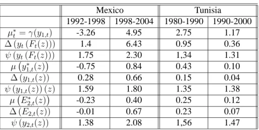
t is set to be equal to the growth rate in the mean income, γ(y1,t), this recession appears to be income equalizing, and could then be described as equitable. To see how this was possible, Table (1) reports the growth rate in the mean income during 1992–1998 as well as many yardsticks of the pro-poorness of this crisis. This table shows that the decline in the mean income of the poor would have been 35 percent higher if Mexico had experienced a counterfactual one-for-one recession pattern. This means that the pace of the rise in poverty, as measured by
(P1,1998(z)), would have been much faster if economic recession had decreased
the income of the poor as much as the income of the non-poor.41 This pro-poor feature of economic recession seems, however, benefitted more the less-so-poor than the poorest of the poor. This is borne out by the values of ψ (yα,1998(z)) (z)
for α = 0 and α = 2 reported in Table (1). The pro-poor index for α = 0 is
(2006) for the Mexican Case.
38The poverty lines selected for the needs of this study are taken from the World Bank (2004)
and Araar et al. (2006) for Mexico and the World Bank (2003) and Bibi and Chatti (2005) for Tunisia. The estimation procedures are very similar since each country applies a version of the share food method.
39More details about this are in Bibi and Chatti (2005) for the Tunisian case and the World Bank
(2004) and Araar et al. (2006) for the Mexican Case.
40On this, see the World Bank (2004).
41This is consistent with other analyses that find relatively lower declines at the bottom of
1.75, whereas it is 1.38 for α = 2, suggesting that economic recession was more ”r-type” than ”p-type” in the Bourguignon and Fields (1997) terminology.
Mexico’s economy has recovered from the peso crisis since 1996. This is demonstrated by the results analysis of the 1998-2004 period reported in Table (1). Growth in the mean income during that period was 4.95 percent per year in average while the annual growth rate needed to achieve the MDGs in terms of headcount reduction is 2.6 percent.42 This impressive growth has more than halved the 1992 headcount ratio. Hence, the natural benchmark growth is then given by µ∗t = 4, 95. As Table (1) reveals, the growth pattern was highly pro-poor since it was associated with positive distributional changes in favor of the poor. For instance, the share of increment to growth captured by the poor pop-ulation is 80 percent higher than that which would have been produced by the benchmark growth pattern (ψ (y1,2004(z)) (z) = 1.8). It is also interesting to note that the value of this pro-poor index is higher for the EDE income resulting from both distribution-sensitive and distribution-insensitive poverty measure, suggest-ing that the larger share of increment to growth captured by the poor has benefitted more those living at the two extremes of the censured distribution.
This pro-poorness feature of the Mexican growth is shared with the Tunisian economy. The mean consumption per capita (γ(y1,t)) in Tunisia grew at an annual rate of 2.75 percent between 1980 and 1990 and 1.17 percent between 1990 and 2000, while the growth rate needed to halve extreme poverty between 1990 and 2015 is 1.1 percent.43 Hence, as in the Mexican case, the benchmark growth is given by µ∗t = γ(y1,t).
During the 1980 – 1990 period, oil export earnings were high, leading to rapid increases in public sector wages and generous subsidies on many foodstuffs. Table (1) shows that these policies were highly pro-poor, since ψ (yα,t(z)) is greater than
1, regardless of the value of α.
Unfortunately, such a pattern of growth was not sustainable since it led to a macroeconomic crisis in 1986. To offset this crisis, the government of Tunisia with the collaboration of the World Bank initiated in the mid-1986 a stabilization program together with structural adjustment reforms.44 As the stabilization pro-gram required the reduction of macroeconomic disequilibria to ensure a sustain-able growth, the government adopted more targeted social expenditures, privatized some public firms, froze public wages, and devaluated exchange rate. Structural
42This growth rate is inferred using equation (3) and the Mexican 1992 income distribution.
43This growth rate is inferred using equation (3) and the Tunisian 1990 household survey.
reforms were applied throughout 1987–1991, but gained increasing importance after 1990.
Many macroeconomic indices showed that these reforms were largely success-ful. While the growth rate in the mean expenditure per capita was less important during the 1990s than the 1980s, Table (1) reveals that the Tunisian ability to con-vert economic growth into pocon-verty reduction is roughly unchanged. For instance, if a 1 percent growth rate led to a 1.35 percent growth rate in the mean income of the poor during the 1980s (ψ (y1,1990(z)) = 1.35), this pro-poorness measure of economic growth rose to 1.38 percent during the 1990s (ψ (y1,2000(z)) = 1.38). Furthermore, the growth pattern targeted more the middle class of the poor dur-ing the 1990s. This can be doubly demonstrated. Firstly, Table (1) shows that ψ (yt(F2000(z))) < ψ (yt(F1990(z))), suggesting that the benefits of economic growth flowed less to the richest of the poor during 1990 – 2000 than during the previous decade. Secondly, the same Table reports a similar result for α = 2,
ψ (y2,2000(z)) < ψ (y2,1990(z)), confirming that the increments to growth were
higher among those who enjoy a level of income close to the mean during the last decade.
Table 1: Pro-poor growth indicators
Mexico Tunisia 1992-1998 1998-2004 1980-1990 1990-2000 µ∗ t = γ(y1,t) -3.26 4.95 2.75 1.17 ∆ (yt(Ft(z))) 1.4 6.43 0.95 0.36 ψ (yt(Ft(z))) 1.75 2.30 1,34 1.31 µ¡y∗ 1,t(z) ¢ -0.75 0.84 0.43 0.10 ∆ (y1,t(z)) 0.28 0.66 0.15 0.04 ψ (y1,t(z)) (z) 1.59 1.80 1.35 1.38 µ¡E∗ 2,t(z) ¢ -0.23 0.40 0.25 0.12 ∆ (E2,t(z)) -0.01 0.67 0.23 0.07 ψ (y2,t(z)) 1.38 2.08 1,56 1.47
Whether these findings are robust to the choice of poverty lines and indices depends on how growth rates are distributed across the population. Figure (1) displays the estimate of the Mexicans’s and Tunisian’s primal growth incidence
different values of the poverty line. The first conclusions that may be drawn from these curves are
• since γ (yt(F1998(z))) is always negative, the distribution of 1992 first-order-dominates (FOD) that of 1998 in Mexico, irrespective of the value of the poverty line. We can then unambiguously conclude that the 1994/1995 Mexican crisis has worsened poverty between 1992 and 1998;
• there is also first order dominance in presence of economic growth both in Mexico and in Tunisia. Thus economic growth has reduced poverty, regard-less of when one set the cut-off point or what poverty index one uses within the class Π1(z) given by equation (20);
• as partial poverty orderings are nested, there is no need to test higher ethical orders to check whether economic growth (crisis) has reduced or worsened poverty.
Turning now to the question of whether economic expansion (contraction) was accompanied by more equity or more inequality, the general conclusions enabled by the complete poverty analysis of the results reported in Table (1) are largely confirmed by the shape of the curves included in Figure (1). Broadly speaking, in presence of economic growth, these curves are decreasing over a large range of poverty lines, showing that the growth pattern is progressive Pen-pro-poor.
This result is confirmed by Figure (3), which proves that during the expan-sion periods in both Mexico and Tunisia, equity gains are larger than those that would have been yielded by the counterfactual growth pattern. During the 1990s in Tunisia, for instance, the growth equity curve taking on an inverted U shape across the bottom of the income, with highest equity growth rates observed at around the pre-selected poverty line. The other curves show a positive and a sharp downward trend for the bottom incomes during the expansion periods. The growth process in both countries has led to a two-edge impact on poverty: increas-ing substantially the income of the poor and reducincreas-ing inequality within the poor. As lower order of dominance entails higher order of dominance, SOD curves in-cluded in Figure (2) are mainly reproduced for illustrative purposes.
The top-left-hand curves of Figure (1) also confirm that the fall in the income of the bottom distribution following the economic crisis experienced by Mexico in 1994/1995 was, for a large range of poverty lines, less important than that in the mean income. Interestingly enough, the primal GIC curve shows a parabolic inverse-U shape around the pre-selected poverty line. This means that while the
income of the poor has decreased less than the average income, it decreases mildly the equality within the poor segment of the Mexican population. The rise in over-all equality reported by the World Bank (2004), for instance, is explained by a rise in equality in the between groups, and not by a rise in equality in the within group of the poor. This is demonstrated by the top-left-hand curves of Figure (3), which show that if we admit that the cut-off point could never be set at 400 percent of the pre-selected poverty standard, the equity growth curve resulting from the crisis lies slightly below that of the counterfactual distributionally neutral crisis. This suggests that the equality measures within the poor fall but this fall is not large enough to offset the rise in equality of the between group.
5
Conclusion
This paper is concerned with the measurement of the extent to which economic growth (or contraction) is distributed amongst the less well-off. For this, com-plete poverty orderings are first used to suggest a new index of pro-poor growth that is devised from a money metric approach and, contrary to the Pernia and Kak-wani (2000) index, goes beyond the measurement of whether growth is equitable. Second, partial poverty orderings are used to extend the poverty-reducing growth framework of Ravallion and Chen (2003) and the inequality-decreasing frame-work of Son (2004) to any degree of ethical dominance. The method can then be used to describe the extent to which growth is poverty-reducing, equitable, and pro-poor for large classes of poverty indices and for ranges of possible poverty lines.
The empirical illustration was achieved by using household surveys from Mex-ico and Tunisia. The calculations show that broadly, economic growth has led to a two-edge impact on poverty: increasing mean income of the poor and reducing income inequality; thus reducing both insensitive and distributional-sensitive poverty indices.
For policy makers concerned with poverty reduction, the aim should certainly be to sustain high growth, but with the poorest capturing a proportionately larger share of the increment to growth. It is obvious that any improvement in distri-bution achieved at the expense of growth would have adverse implications for poverty reduction. Yet is there any trade-off between equity, poverty reduction, and efficiency? There is plenty of evidence to suggest that countries with more unequal income distribution have lower growth. When extreme inequalities rein-force poverty, they act as a barrier to growth by restricting the productive potential,
undermining investment, and limiting the capacity of a large section of the popu-lation from responding to incentives created through market reforms. Put bluntly, pro-rich growth is not only bad for social justice, it is also bad for economic ef-ficiency. In this paper, the properties of pro-poor growth are characterized by suggesting pro-poor poverty indices that truly capture the pro-poorness of growth according to different ethical principles. The next challenge is to establish which types of policy reforms are more likely to achieve both high and equitable growth.
References
[1] Araar, A., J.-Y. Duclos, P. Makdissi, and M. Audet (2006), Pro-Poor Economies and Statistical Robustness: Evidence Using Mexican Data.
Mimeo, University of Laval, Quebec, Canada.
[2] Atkinson, A. B. (1970), On the Measurement of Inequality, Journal of Eco-nomic Theory, vol. 2, pp. 244–263.
[3] Atkinson, A. B. (1987), On the Measurement of Poverty. Econometrica, vol. 55 (4), pp. 749–764.
[4] Bhagwati, J. N. (1988), Poverty and Public Policy. World Development, vol. 16 (5), pp. 539–554.
[5] Besley, T. and R. Kanbur. (1993), The Principles of Targeting. In: Michael Lipton and Jacques Van Der Gaag (eds), Including the Poor, The World Bank, pp. 67-90.
[6] Bibi, S. (2002), Does the Specification of a New Class of Poverty Measures Matter? Evidence from Tunisia. Paper presented at the 27th General Con-ference of the International Association for Research in Income and Wealth, Stockholm, August 18 - 24, 2002, Sweden.
[7] Bibi, S. and R. Chatti (2005), Public Spending, Pro-poor Growth and Poverty Reduction in Tunisia: A Multilevel Analysis. The Arab Planning Institute, Kuwait.
[8] Bibi, S. and J.-Y. Duclos (2005), Decomposing Poverty Changes into Verti-cal and Horizontal Components. Bulletin of Economic Research. vol. 57 (2), pp. 205–215.