HAL Id: hal-00655390
https://hal.archives-ouvertes.fr/hal-00655390
Submitted on 8 Jan 2012HAL is a multi-disciplinary open access
archive for the deposit and dissemination of sci-entific research documents, whether they are pub-lished or not. The documents may come from teaching and research institutions in France or abroad, or from public or private research centers.
L’archive ouverte pluridisciplinaire HAL, est destinée au dépôt et à la diffusion de documents scientifiques de niveau recherche, publiés ou non, émanant des établissements d’enseignement et de recherche français ou étrangers, des laboratoires publics ou privés.
Estimation of the 3D self-similarity parameter of
trabecular bone from its 2D projection
Rachid Jennane, Rachid Harba, Gerald Lemineur, Stépahnie Bretteil, Anne
Estrade, Claude-Laurent Benhamou
To cite this version:
Rachid Jennane, Rachid Harba, Gerald Lemineur, Stépahnie Bretteil, Anne Estrade, et al.. Estimation of the 3D self-similarity parameter of trabecular bone from its 2D projection. Medical Image Analysis, Elsevier, 2007, 11 (1), pp.91-98. �10.1016/j.media.2006.11.001�. �hal-00655390�
Estimation of the 3D self-similarity parameter of
trabecular bone from its 2D projection
Abstract
It has been shown that the analysis of two dimensional (2D) bone X-ray images based on the fractional Brownian motion (fBm) model is a good indicator for quantifying alterations in the three dimensional (3D) bone micro-architecture. However, this 2D measurement is not a direct assessment of the 3D bone properties. In this paper, we first show that S3D, the self-similarity parameter of 3D fBm, is linked to S2D, that of its 2D projection, by S3D = S2D - 0.5. In the light of this theoretical result, we have experimentally examined whether this relation holds for trabecular bone. Twenty one specimens of trabecular bone were derived from frozen human femoral heads. They were digitized using a high resolution -CT. Their projections were simulated numerically by summing the data in the three orthogonal directions and both 3D and 2D self-similarity parameters were measured. Results show that the self-similarity of the 3D bone volumes and that of their projections are linked by the previous equation. This demonstrates that a simple projection provides 3D information a bout the bone structure. This information can be a valuable adjunct to the bone mineral density for the early diagnosis of osteoporosis.
Keywords: Self-similarity; fractional Brownian motion; fractal; trabecular bone; osteoporosis; X-ray images;
computed tomography.
Rachid JENNANEa,*, Rachid HARBAa, Gérald LEMINEURa, Stéphanie BRETTEILa, Anne ESTRADEb and Claude Laurent BENHAMOUc
a
Laboratory of Electronics, Signals and Images, GDR-ISIS, Université d’Orléans, BP 6744, 45067 Orleans, Cedex 2 FRANCE.
b
Laboratory of Mathematics and Applications of Paris 5, University René Descartes 45, rue des Saints-Pères, 75270 Paris Cedex 06, FRANCE
c
1. Introduction
Osteoporosis is characterized by low bone mass and micro-architectural deteriorations of bone tissue (Parfitt, 1992). These modifications lead to enhanced bone fragility, and consequently increase the risk of fracture (Consensus Development Conference, 1991). The distribution of mineral content in three dimensions, and the loading of the skeleton are additional factors that contribute to bone fragility.
The diagnosis of osteoporosis is mainly based on dual energy X-ray absorptiometry which amounts to measuring bone mass. Characterization of the trabecular structural properties appears to be an important adjunct to the measurement of bone mass in determining fracture risk with greater accuracy (Goldstein, 1987). Using histological and stereological analysis, it has been shown that, by combining structural features with bone density, nearly all of the variability in mechanically measured Young’s moduli could be explained (Goulet et al., 1994; Croucher et al., 1996). However, the evaluation of bone structure, by non- invasive procedures, remains a difficult issue (Faulkner et al., 1991).
Bone X-ray radiographs have been suggested as a means of quantifying trabecular changes (Rockoff et al., 1986; Aggarwal et al., 1986). This method shows potential as we know that radiographs are feasible and are not life threatening. Among many methods that can extract the information from natural images, fractals are efficient candidates (Pentland, 1984), and fractional Brownian motions (fBm) (Mandelbrot and Van Ness 1968) are widely used. FBm is governed by the single Hurst parameter, H (0 < H < 1). It has been shown that H and the intuitive notion of roughness are closely linked: the lower H is, the higher is the roughness (Pentland, 1984). Concerning bone radiographs, this idea was used in (Lundhal et al., 1986) to characterize the texture roughness. It was shown that H follows the clinically expected course of osteoporosis closely, in that a lower H indicates a greater degree of osteoporosis. Indeed, during osteoporosis, trabeculae become thinner, perforations occur, and some of the fine trabecular structures are broken. Radiographs appear naturally rougher, leading to a decrease in H. These results have been confirmed by subsequent studies (Benhamou et al., 1994; Majumdar et al., 1997; Majumdar et al., 2000; Prouteau, 2004). Clinical results have also pointed out the strong potential
of the H parameter of fBm in quantifying osteoporosis on bone X-ray radiographs (Pothuaud et al., 1998; Lespessailles et al., 1998).
An X-ray radiograph is a two-dimensional (2D) projection of a three-dimensional (3D) structure. The difficulty in using such 2D projectio ns is in determining exactly how the 2D parameters measured on radiographs are related to 3D ones. This problem is part of the more general one of using 2D images, either slices or projections, to characterize 3D materials. This is a difficult issue, though some results are available in the case of fractals. For example, it is well known that a 2D slice of a fractal volume has the same H parameter as the volume itself (Mandelbrot, 1982). However, for projections, no equivalent link has been established. One way to elucidate the problem is to conduct experimental studies on real material (Pothuaud et al., 2000; Jennane et al., 2001; Guggenbuhl et al., 2006). However, this approach which consists in estimating 3D properties from 2D projections suffers from the lack of a strong theoretical background. Moreover, the relations between 2D and 3D parameters remain unclear.
Recently, an isotropic analysis for Gaussian models having stationary increments has been suggested (Bonami and Estrade, 2003). This study was applied in (Jennane et al., 2001) where we proposed an oriented fractal analysis for anisotropic fractional Brownian motion. The theoretical study presented in (Bonami and Estrade, 2003) can also be applied to 3D bone images. In this paper, we first establish a formal link between S3D, the self-similarity of a 3D continuous fBm process and S2D, the
self-similarity of its 2D projection, that is S2D = S3D + 0.5. In the light of this theoretical result, we
experimentally examine whether or not this formal link holds for trabecular bone. With this aim in view, we study high resolution micro computed tomography (-CT) images and simulate their 2D projections obtained by summation of the voxels of the 3D structure. Then, 2D and 3D self-similarity parameters are measured and compared. If the formal link S2D = S3D + 0.5 holds for trabecular bone, information on
3D structure can be extracted out of 2D radiographs and can help in the early diagnosis of osteoporosis. The paper is organized as follows: In section II, we de monstrate the relation between 3D and 2D self-similarity parameters for fBm. Section III presents the preparation and acquisition of the μ -CT bone images. The measurement methods for 3D and 2D self-similarity descriptors are explained in section IV. Section V presents the results and we conclude with a brief discussion of this work.
2. Theory
It has been shown that the H parameter of the fBm is a good indicator for the alterations of the 3D bone micro-architecture seen on 2D bone radiographs (Benhamou et al., 1994; Majumdar et al., 1997). However, this 2D measurement is not a direct assessment of the 3D bone properties. Based on a recent paper (Bonami and Estrade, 2003), it is possible to establish a formal link between S3D, the
self-similarity of a 3D continuous fBm and S2D, the self-similarity of its 2D projection. The aim of this
section is to demonstrate this relation.
Let us first recall a result and the way to obtain it. We are interested in a signal indexed by the position in the 3D space domain, given by a fBm, BH : (BH(x); x in R3). One of the characteristics of
fBm is self-similarity, that is to say:
for all scales (non-negative),
B ( x);x3
B (x);x3
HH
H , (1)
where means equal in distribution. The Hurst parameter H is also the 3D self-similarity index denoted, S3D. Thus, S3D = H.
The self-similarity identity (1) can be obtained as follows. Since BH is a zero mean Gaussian field
with stationary increments, its distribution is completely defined by the variance of its increments
BH(x): 3 2 in x all for , )) ( (BH x x H Var , (2)
where, for a multidimensional lag x at any point x0 in 3,
). ( ) ( ) (x B x0 x B x0 BH H H (3)
2 3 2 2 2 1 3 2 1 for x (x, x,x ) , x x x x . (4)
Now, introducing a change of scale xx gives the following:
)) ( ( )) ( ( B x x 2 2 x 2 2 Var B x Var H H H H H H , (5) which shows (1).
In the following, the term projection will be used for a simple sum of the planes of the 3D structure. To establish the formal link between the self-similarity of a 3D fBm and that of its 2D projection, we will now consider the projection along one of the three orthogonal directions. This direction plays a special role and we will denote for clarity x = (x1, x2, z), x 3 the 3D position in the space domain
where z is the projection direction. Identically, = (1,2,z), 3 is the 3D position in the frequency
domain. When BH is projected along the z axis, one obtains a 2D Gaussian field YH:
B x x z z dz x x YH( 1, 2) H( 1, 2, )( ) . (6)(z) is a window that ensures the convergence of the previous integral. YH is no longer a fBm but still
has stationary increments as proved in the following. Consider the spectral representation of a 3D fBm (Reed et al., 1995):
3 2 2 1 1 , , ) , , ( 1 1 ) , , ( 1 2 2 3 2 1 ) ( 2 1 z H z z x x i H H dW e C z x x B z , (7)where CH is a non negative constant and dW is a 3D Brownian measure in frequency. The projected
field can be represented as follows:
3 2 2 1 1 , , ) ( ˆ ) , , ( 1 1 ) 0 , 0 ( ) , ( ) , ( 1 2 2 3 2 1 ) ( 2 1 2 1 z z H z x x i H H H H dW e C Y x x Y x x Y , (8)where ˆ is the Fourier transform of . Computing the variance of YH we obtain
. 1 ) ( ˆ ) ( 2 1 sin 1 )) , ( ( 2 2 1 2 3 2 2 2 2 1 2 2 2 1 1 2 2 H 2 1
x d d d x C x x Y Var z H z z H (9)This variance does not satisfy any identity such as (5) and therefore the projected field YH is not
self-similar. However, we are going to demonstrate that YH is self-similar for small scales.
Let us determine the variance of YH(x1, x2). Introducing the change of variable
1,2
1,2
in the integral above, we get:
. 1 ) ( ˆ ) ( 2 1 sin )) , ( ( 2 2 1 2 3 2 2 2 2 2 1 2 2 2 1 1 2 2 1 2H 2 1
x x d d d C x x Y Var z H z z H H (10)For small scale , i.e. 0, and if H < 0.5:
H 0.5 H 2 2 1 2 2 3 2 2 2 1 2 2 1 1 2 2 H 1 2H 2 1 ˆ( ) 1 ) ( 2 1 sin C )) , ( ( 2 V d d d x x x x Y Var z z H H
(11)where VH is a constant which does not depend on . In that case, by analogy with identity (5), we say
that YH is asymptotically self-similar of index H + 0.5. In other words, S2D = H + 0.5. Actually, the
previous result is only valid for H < 0.5. For H > 0.5, the result still remains true when using the 2-order increments of YH, that is to say
H 1 2H 2 V )) ( ( Y x Var H , (12) where ), ( ) ( 2 ) 2 ( ) ( 2 x Y x x Y x x Y x Y o o (13)
with V’H a constant which does not depend on . The latter equation is valid for any point xo in 2.
Hence, the asymptotical self-similarity index of the projection YH which is a 2D signal process is
S2D = H + 0.5 while the self-similarity index of the original 3D process is S3D = H. For small scale , we
can write that:
0.5. S
S3D 2D (14)
Several remarks can be made at this point.
Remark 1: Although this result has been shown in the 3D case, it is valid for any space dimension above one.
Remark 2: The increase in the self- similarity of the projection is not unexpected since this operation is an integration process. This action leads to softer objects, thus increasing the self-similarity index. Remark 3: For the main result (14) to be valid, the self-similarity parameter of the projection should be estimated for small scales , or in other words for high frequency. The practical estimation of S2D
Remark 4: The projected process is not self-similar but asymptotically self- similar at high frequency of index H + 0.5 in the interval ]0.5, 1.5[. For the large scale domain, i.e. the low frequency domain, it ca n be shown that the projected process YH is asymptotically self-similar of parameter H (Bonami and
Estrade, 2003). As a conclusion, YH has 2 different asymptotical self-similar parameters, H at low
frequency and H + 0.5 at high frequency.
We will now explore if this theoretical result holds for 3D trabecular bones and their 2D projection. The next paragraph explains how the bone samples were acquired and digitized.
3. Preparation and acquisition of bone specimens
A total of 21 frozen human femoral heads were used to derive 21 specimens of trabecular bone. Cylindrical samples were prepared under continuous water irrigation using a precision diamond circular saw. The samples were oriented with respect to anatomic axes and cut to a dimension of 6 mm thickness and 8 mm diameter. All the samples were defatted chemically (several cycles of submerging in dichloromethane).
Images were obtained using the Skyscan 1072 high-resolution -CT. The X-ray source was set at 80kV and 100µA, and the magnification was fixed to get a pixel size of 12 µm. A 10241024 12-bit digital cooled CCD coupled to a scintillator was used to record the radiographic projections. 209 projections were acquired over an angular range of 180° (angular step of 0.9°). Due to the cone beam the radiographic images were processed with the Feldkamp algorithm. The exposure time for one radiographic projection was about 5.9s so that the total scan for each sample lasted 1 hour. All the radiographic images were transferred to a personal computer (PIII, 933MHz) and the image slices were reconstructed using the conebeam reconstruction software version 2.6.
We used the central part of each image which is 4.80 mm3, equivalent to 4003 pixels. Fig. 1 shows two such cubes having different 3D structures.
(a) (b) Fig. 1. two 3D specimens.
The differences between these two samples are obvious: low density and connectivity for Fig. 1a, high density and connectivity for Fig. 1b. This is confirmed by the following:
- BV/TV (the ratio between the volume of trabecular bone (BV) and the total volume (TV)) was 0.182 for sample (a) and 0.306 for (b)
- Conn.D (the connectivity density parameter) was -0.0044 for sample (a) and -0.0075 for (b).
- For the 21 samples, the mean and standard deviation for BV/TV was 0.210 0.066, and -0.0111 0.0096 for Conn.D.
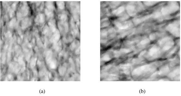
We now wish to compute the projection of these bone volumes. To do so, we used a simple projection which consists of summing the data in the three orthogonal directions x1, x2 and z. Fig. 2
illustrates two projections along the z axis of the two bones presented in Fig. 1. z
x1
(a) (b)
Fig. 2. Two projections along the z-axis for the two specimens presented in Fig. 1.
As can be seen, the projection of the bone volumes generates grey level images. It is also noticed that image 2.a is different from image 2.b as is the case for the bone volumes of Fig. 1. It is then expected that the 3D self- similar parameter and that of its 2D projection are linked.
Our aim is to apply to a binary object (trabecular bone) a result concerning the relation between 3D and 2D self-similarity demonstrated using a continuous fractal model (fBm). A better approach would be to use a 3D binary fractal model indexed by R3 taking values in {0, 1}. At this point of our project, such work is under active investigation. We hope that in a near future we will be able to propose such a result for some class of binary fractals.
We will now present the chosen tools to access the self- similarity of these 3D and 2D images.
4. Measure ment of 2D and 3D self-similarity
A wide variety of computer algorithms for estimating the fractal index of a structure exist. The most widely used algorithms in signal and image processing are described in (Barnsley et al., 1988; Jenna ne et al., 1996, 2001).
4.1. 2D self-similarity: the variance method
The projections of 3D bones are 2D grey level images as seen on Fig. 2. Thus equation (5) can be applied to assess the 2D self-similarity. This method is known as the variance method of Pentland (Pentland, 1984). It requires that the increments I(x) of the grey levels I(x) be computed for different lags . If self-similar of index S2D, the following relation holds:
)) ( ( )) ( ( I x 2 2 Var I x Var S D , (15)
where x is a position index.
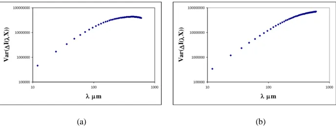
In this case, the Log-Log plot of Var(I(x)) versus is a straight line of slope 2S2D. Such
representations for the variance of the grey level increments obtained over images lines presented in Fig. 2 are illustrated on Fig. 3. Note that corresponds in the discrete case to the number of pixels considered for the lag’s increment. For example, for the 8 first points the spatial resolution varies between 12 μm and 96 μm. 100000 1000000 10000000 100000000 10 100 1000 m V ar ( I( X )) 100000 1000000 10000000 100000000 10 100 1000 m V ar ( I( X )) (a) (b)
Fig. 3. Log-Log plot of the variance of the increments versus the lag for the two projections of Fig. 2.
It should be remembered that, even if the 3D structure is self- similar, the projected field is only asymptotically self-similar at small lags . This is typically what we observe. For that reason, we
choose to estimate S2D over the first eight points of the Log-Log plot which show a fair linearity. This
area characterizes the bone structure at the trabecular thickness scale (Harba et al., 1994). Knowing that the pixel size is about 12 m defines physically a lag whose size is 96 m. This ensures a lag of measure lower than the trabecular size (about 100 to 200 m for the bigger trabeculae) and allows an examination of what is going on inside the trabecular structure to detect perforation or rupture of the trabeculae. S2D was computed as the mean value of the 400 values estimated over 400 lines of each image.
4.2. 3D self-similarity: the box counting method
The self-similarity of a continuous object, as for example our 2D images, is easily assessed using equation (5). However, concerning our application, it is obvious that 3D trabecular bone is not a continuous object, but rather a binary one. Nevertheless, the notion of self- similarity does exist for such data. Binary fractals are unusual geometric structures that can be used to analyze many biologic structures not amenable to conventional analysis. The full-sized object is composed of elements, these elements composed of the same elements even smaller, and so on down to the microscopic level. Trabecular bone has a branching pattern, as seen on Fig. 1. One can also see that it exhibits self-similarity, that is the trabeculae and the narrow spaces between them look very similar no matter what their size.
The notion of self-similarity is linked to the volume of the structure defined by the following: the original 3D structure is regularly cut in sma ll cubes, or in boxes, of size ρ. The number N(ρ) of boxes containing at least one mineral element is evaluated. The corresponding volume V(ρ) is given by:
3 ) ( ) ( N V (16)
If a binary structure is self-similar of index S3D then the following relation holds for any scale index
> 0: ) ( ) ( 3 V V SD . (17)
Rewriting V(ρ) from (16) and replacing V(ρ) in equation (17), as a consequence, it easily results that N(ρ) is proportional to (3S3D)
. Returning to fractal objects, the relation between N(ρ) and ρ is (Falconer, 1987):
D C
N() . (18)
where D is the fractal or box dimension of the object and C a constant. Thus, by combining this result with previous ones, the self-similar parameter S3D is linked to D by:
D
S3D 3 . (19)
This analysis is called the box counting method. The idea that the fractal dimension of trabecular bone might be related to bone architecture and bone strength is an appealing one, since the fractal dimension can be assessed from clinical images.
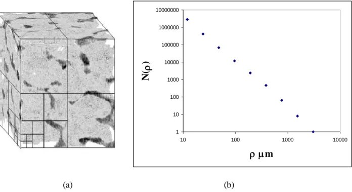
Fig. 4 shows a bone volume specimen with d ifferent boxes’ edges and the corresponding Log-Log plot of N(ρ) versus ρ. The fractal dimension is easily estimated from this figure and S3D results from the
last equation.
To avoid the phenomenon of length described in (Tricot et al., 1988; Feder, 1988), the size of the boxes varies by a power of 2. To be consistent with the measure of S2D, the slope was measured on the
fourth first points of each Log-Log plot which corresponds to a spatial resolution between 12 μm and 96 μm.
1 10 100 1000 10000 100000 1000000 10000000 10 100 1000 10000 m N( ) (a) (b)
Fig. 4. (a) A 3D bone volume with several grids placed over the bone structure, and (b) the Log-Log plot of N(ρ) versus ρ for the bone volume specimen.
For both 2D and 3D analysis, the image files were processed with custom designed software developed at our institution using Microsoft Visual C++ language.
5. Results
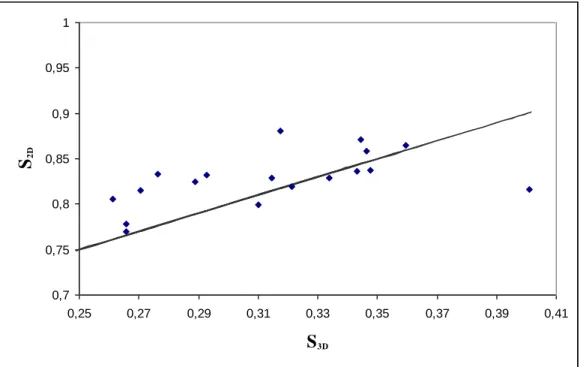
Both 2D and 3D self-similarity indices were estimated on the 21 bone volumes and on their projections using the above methods. We examined experimentally if these parameters are linked by S3D = S2D - 0.5 as is the case for continuous fBm. Fig. 5 shows as an example the evolution of S2D along
0,7 0,75 0,8 0,85 0,9 0,95 1 0,25 0,27 0,29 0,31 0,33 0,35 0,37 0,39 0,41 S3D S2D
Fig. 5. Representation of S2D along the z-axis versus S3D for the 21 bone samples, as well as the straight
S2D = S3D + 0.5.
We notice that S2D and S3D are not far from being related by S2D = S3D + 0.5. To confirm this
tendency, the mean offset, S2D - S3D, and its standard deviation are presented for the three orthogonal
directions x1, x2 and z in Table 1.
Table 1
Mean and standard deviation for S2D - S3D along the three orthogonal directions computed on the 21
bone cubes. S2D - S3D along the x1-axis S2D - S3D along the x2-axis S2D - S3D along the z-axis mean 0.551 0.533 0.518 Standard deviation 0.043 0.039 0.034
This confirms that the above relation is true for trabecular bone. It provides an interesting tool to quantify the 3D architecture from its two dimensional projection. The main advantage is that 2D bone radiographs are not life threatening, cheap and easily obtainable.
6. Conclusion
In the light of a new theoretical result shown in this paper, this study on high resolution μ -CT bone images has aimed to establish the possible links between the self-similarity of 3D bone volumes and that of their 2D projections. Results show that it is feasible to access the self-similarity of 3D bone volumes solely from their projections computed numerically by summing the original data in the three orthogonal directions. The object of such investigations is a crucial issue to assess changes in bone structure only from 2D X-ray bone radiographs which is cheap and not life threatening. This evaluation of bone micro-architecture may be a useful indicator in a variety of tasks of clinical interest, especially in the prediction of diseases such as osteoporosis. Beyond its application to bone, this result may be interesting for other porous materials. This study opens the way to further theoretical and practical developments.
First, the relation between the three and two-dimensional self-similarity has not been shown for binary fractals. Moreover, it will be interesting to establish a formal link between the self-similarity and the connectivity of the bone which is one of the most useful parameters to assess bone strength. To address these two theoretical issues, we are considering binary self-similar models that can be used for such investigations.
Second, we have shown that the 2D projection of 3D fBm of H parameter in ]0, 1[ is asymptotically self-similar of parameter H at low frequency and asymptotically self-similar of parameter H + 0.5 at high frequency. Hence, the 2D projection of a 3D fBm is a natural example of the generalized model proposed in (Kaplan and Kuo, 1994; Perrin et al., 2005) taking into account this piecewise behavior. This theoretical background justifies a local measurement of the H parameter as well as a value of the self-similarity index that takes values above 1. This new approach could be used for a better assessment of the H parameter of bone radiographs.
Finally, from a practical point of view, we are actively developing a high resolution digital X-ray bone prototype at a pixel size of 50 μm which will be used for the clinical evaluation of bone architecture. By associating these theoretical and practical advances, and combining both micro-architecture and density parameters of the bone, we believe that the early and efficient diagnosis of osteoporosis will be achieved within the next few years.
References
Aggarwal N. D., Singh G. D., Aggarwall R., 1986. A survey of osteoporosis using the calcaneum as an index. Int. Orthop., Vol. 10, pp. 147-153.
Barnsley M. F., Devaney R. L., Mandelbrot B. B., Peitgen H. O., Saupe D., Voss R. F., 1988. The Science of Fractal Images. Springer Verlag, New York.
Benhamou L., Lespessailles E., Jacquet G., Harba R., Jennane R., Loussot T., Tourliere D., Ohley W. J., 1994. Fractal Organization of the Trabecular Bone Images on Calcaneus Radiographs. Journal of Bone Mineral Research, Vol. 9, pp. 1909-1918.
Bonami A., Estrade A., 2003. Anisotropic Analysis of some Gaussian Models. The Journal of Fourier Analysis and Applications, Vol. 9, pp. 215-236.
Consensus Development Conference, 1991. Diagnosis, Prophylaxis and Treatment of Osteoporosis. Am J. Med., pp. 107-10, 1991.
Croucher P. I., Garrahan N. J., Compton J. E., 1996. Assessment of cancellous bone structure: comparison of strut analysis, trabecular bone pattern factor, and narrow space star volume. J. Bone. Miner. Res, Vol 11, pp. 955-961.
Falconer K. J. , 1985. The Geometry of Fractal Sets. Cambridge University Press, Cambridge.
Faulkner K. G., Gluer C. C., Majumdar S., Lang P., Engelke K., Genant H. K., 1991. Noninvasive Measurements of Bone Mass, Structure and Strength: Current Methods and Experimental Techniques. AJR, Vol. 157, pp. 1229-1237.
Feder J., 1988. Fractals, Plenum Press, New York and London.
Goldstein S. A., 1987. The Mechanical Properties of Trabecular Bone: Dependence on Anatomic location and Function. Journ. Biomech, Vol. 20, pp. 1055-1061.
Goulet R. W., Goldstein S. A., Ciarelli M. J., Kuhn J. L., Brown M. B., Feldkampt L. A., 1994. The relation between the structural and orthogonal compressive properties of trabecular bone. J. Biomechanics, Vol. 27, pp. 375-389.
Guggenbuhl P., Bodic F., Hamel L., Basle M. F., Chappard D, 2006. Texture analysis of X-ray radiographs of iliac bone is correlated with bone micro-CT. Osteoporos Int., Vol. 17, N° 3, pp. 447-457.
Harba, G. Jacquet, R. Jennane, T. Loussot, C. L. Benhamou, E. Lespessailles, D. Tourlière, 1994. Determination of Fractal Scales on Trabecular Bone X-Ray Images. Fractals, Vol. 2, N° 3, pp. 451-456.
Jennane R., Harba R., Jacquet G., 1996. Quality of Synthesis and Analysis Methods for Fractional Brownian Motion. IEEE Digital Signal Processing WorkShop, Loen, Norway, pp. 307-310.
Jennane R., Harba R., Jacquet G., 2001. Méthodes d’analyse du mouvement brownien fractionnaire: théorie et résultats comparatifs. Traitement du Signal, Vol. 18, N° 5-6, pp. 419-436.
Jennane R., Harba R., Perrin E., Bonami A., Estrade A., 2001. Analyse de champs browniens fractionnaires anisotropes, GRETSI 2001, pp. 99-102.
Jennane R., Ohley W. J., Majumdar S., Lemineur G., 2001. Fractal Analysis of Bone X-Ray Tomographic Microscopy Projections. IEEE Tans. on Med. Imag., Vol. 20, N° 5, pp. 443-449. Kaplan L. M., Kuo J. C. C., 1994. Extending Self-Similarity for Fractional Brownian Motion. IEEE
Trans. on Signal Proc., Vol. 42, N° 12, pp. 3526-3550, 1994.
Lespessailles E., Jullien A., Eynard E., Harba R., Jacquet G., Ildefonse J. P., Ohley W., Benhamou C. L., 1998. Biomechanical Properties of human os calcanei : relationships with bone density and fractal evaluation of bone microarchitecture. Journal of Biomechanics, Vol. 31, pp. 817-824. Lundhal T., Ohley W. J., Kay S. M., Siffert R., 1986. Fractional Brownian motion : a maximum
likelihood estimator and its application to image Texture. IEEE Transactions on Medical Imaging, vol. 5, pp. 152-161.
Majumdar S., Link T. M., Ouyang X., Milard J., Lin J. C., Tsag D., 1997. Fractal Analysis of Radiographs: Comparison of Techniques and Correlation with BMD and Biomechanics. Journal of Bone Mineral Research, Vol. 12, T652.
Majumdar S., Link T. M., Millard J, Lin J. C., Augat P., Newitt D., Lane N., Genant H. K., 2000. In vivo assessment of trabecular bone structure using fractal analysis of distal radius radiographs. Med. Phys., Vol. 27, N° 11, pp. 2594-2599.
Mandelbrot B. B., Van Ness J., 1968. Fractional Brownian Motion, Fractional Noise and Applications. SIAM, Vol. 10, pp. 422-438.
Mandelbrot B. B., 1982. The fractal geometry of nature. W. H. Freeman, San-Fransisco.
Odgaard A., Gundersen H. J. G., 1993. Quantification of Connectivity in Cancellous Bone, With Special Emphasis on 3D Reconstructions. Bone, Vol. 14, pp. 173-182.
Parfitt A. M., 1992. Implications of Architecture for the Pathogenesis and Prevention of Vertebral fractural. Bone, Vol. 13, Suppl2, pp. 41-77.
Pentland A. P., 1984. Fractal- Based Description of Natural Scenes. IEEE Trans. on Patt. and Mach. Int., Vol. PAMI-6, N° 6, pp. 661-674.
Perrin E., Harba R., Jennane R., Iribarren I., 2005. Piecewise fractional Brownian motion. IEEE Transactions on Signal Processing, Vol. 53, N°. 3, pp. 1211-1215.
Pothuaud L., Lespessailles E., Harba R., Jennane R., Royant V., Eynard E., Benhamou C. L., 1998. Fractal Analysis of trabecular Bone Texture on Radiographs: Discriminant value in post menopausal Osteoporosis. Osteoporosis International, Vol. 8, pp. 618-625.
Pothuaud L., Benhamou C. L., Poirion P., Lespessailles E., Harba R., Levitz P., 2000. Fractal Dimension of Trabecular Bone Projection Texture Is Related to Three-Dimensional Microarchitecture. Journal of Bone and Mineral Research, Vol. 15, N° 4, pp. 691-699.
Prouteau S., Ducher G., Nanyan P., Lemineur G., Benhamou L., Courteix D., 2004. Fractal analysis of bone texture: a screening tool for stress fracture risk?, Eur J Clin. Invest. Vol. 34, N° 2, pp. 137-142.
Reed S., Lee P., Truong T. K. , 1995. Spectral Representation of Fractional Brownian Motion in n Dimensions and its Properties. IEEE Trans. on Inf. Theory, Vol. 41, N° 5, pp. 1439-1451.
Rockoff S. D., Scandrett J., Zacher R., 1971. Quantitation of relevant image information : automated radiographic bone trabecular characterization. Radiology, Vol. 101, pp. 435-439.
Simmons C. A., Hipp J. A., 1997. Method Based Differences in the Automated Analysis of the Three-Dimensional Morphology of Trabecular Bone. Journal of Bone and Mineral Research, Vol. 12, N° 6, pp. 942-947.
Tricot C., Quiniou J. F., Wehbi D., Roques-Carmes C., Dubuc B., 1988. Evaluation de la dimension fractale d’un graphe. Revue Phys. Appl., Vol. 23, pp. 111-124.