Design and Use of In-process Sensing and Adaptive Compensation in Flexible Assembly
by
David N. Beal BS, Mechanical EngineeringCornell University, 1995
Submitted to the Department of Mechanical Engineering in Partial Fulfillment of the Requirements for the
Degree of Master of Science
at the Massachusetts Institute of Technology January 1997
@ Massachusetts Institute of Technology, 1997 All rights reserved
Signature of Author
Department of Mechanical Engineering January 18, 1997
Certified By
Professor David Hardt Thesis Supervisor
Certified By
Professor Ain A. Sonin Department Committee on Graduate Studies
OF TECtH".
Design and Use of In-process Sensing and Adaptive Compensation in Flexible Assembly
by
David N. BealSubmitted to the Department of Mechanical Engineering on January 30, 1997, in Partial Fulfillment of the Requirements
for the Degree of Master of Science
Abstract
As product lifetimes get shorter, the traditional assembly lines exclusive to one product are becoming increasingly cumbersome, in both start-up time and cost. Consequently,
industry is moving towards flexible assembly: an automated line that can produce any product in a class with a minimum of changeover time between products. It was desired to design, build and test a flexible assembly line for a specified class of products, in order to identify the issues associated with assembly of these products, and to develop
innovative solutions to these issues.
This thesis discusses the evolution of the design of the assembly line. The design of the transport module is then discussed, with issues of speed, precision, strength, locating, and ease in line adjustment or upgrading. A final transport module design is then presented. It was then desired to build and test some of the more ambitious and innovative aspects of the design, specifically those which involve part-referenced measurement. Results from an optical hole-finding method are discussed. A novel compliant pin locating device, using force and displacement information of the bent pin, is then presented and characterized.
Acknowledgments
The author would like to thank, in no certain.order:
Ken and Carole Beal, Doug, Tricia, and Stuart, Steve and Beth, the Grandparents, and the whole extended family, for your unconditional support throughout. You are a wonderful family and I owe you more than I can give.
Professor David Hardt for giving me the guidance and advice that I needed to get me through, both in academia and out.
Ivan, Brian, Steve, Wes, Sieu, Kian, Jeremy, Guvenc, Wayne, Dave, and all the kids in the lab for the camaraderie, humor, and slight insanity.
Niraj, Steve, Hettie, Peter, James, Jason, Eddie, and Paul for keeping me well distracted from my studies in Boston.
Jeff, Roman, Mark, Matt for being the bad influences I needed during my developing years. I wish you all the best during your journeys.
Fred Cote for the unlimited advice and availability. I don't know how far I'd have gotten without it.
Keith Drumheller and Tom Davis for their patience, guidance, and leadership.
Table of Contents
Introduction Chapter 1 Chapter 2 Section 2.1 Section Section Section 2.2 Section 2.3 Chapter 3 Section 3.1 Section 3.2 Section 3.3 Section 3.4 Chapter 4 Section 4.1 Chapter 5 Chapter 6 Chapter 7 Section 7.1 Section 7.2 Section 7.3 Section 7.4 Chapter 8 Section 8.1 Section 8.2 Section 8.3 Section 8.4 Chapter 9 Section Section Section Section Section Chapter 10 References Appendix A Appendix B Appendix C 2.1.1 2.1.2 9.1 9.2 9.3 9.4 9.5 .. .. ... .... .. . ... ... ... 9Assembly Line Design ... ... 12
Transport Module Design... 16
Speed and Precision... ... 17
Redundant X-axis... ... 18
D ocking... 19
Actuator and Structure Strength... 20
Gripping and Locating... ... 21
Transport Module Details... 26
Axis Orientation... ... 26
Docking... . ... 28
Transport... 34
Rover Design... ... 36
The Final Design... . .... ... 42
The Experimental Testbed ... 44
Part Referenced Measurement and Control... 50
H ole Finding...,... 55
Coplanarity Detection and Compensation Design... 67
Contact Probe... ... 70
Non-contact Electrical Methods... 71
Optical Methods... 73
Force-Displacement Methods... 76
Piezo Probe Design... ... 84
Noise and Drift... 86
Probe Redesign... ... ... 90
D ata-A veraging... 94
Probe Test... ... 95
Coplanarity Detection, Compensation, and Process Characterization... 98
Electronics... .... ... 102
Probe ... 109
Materials ... 109
Geom etry... ... 111
Location Detection -Experimental Results... 116
Closing Remarks ... ... ... 120
... ... ... 12 2 Improvements to the Serial Insertion Module... 124
Coupling Load Spreadsheet... 130
List of Figures
Figure 1.1: Example housing... ... ... .... ... 12
Figure 1.2: A ssem bly line layout... ... 13
Figure 1.3: Bending Module interfacing with Manipulator on Transport Module... 14
Figure 1.4: Iterative algorithm used for bending parts with the bending module... 15
Figure 2.1: The axis orientation relative to a housing... 17
Figure 2.2: The simple 4-axis system showing definitions of axes... 17
Figure 2.3: The redundant X-axis system for coarse and fine motion... . 19
Figure 2.4: Front Pull Assisted Y-axis System... ... 21
Figure 2.5: Shows the backlight, photodetector, and grippers... 23
Figure 2.6: Shows gripper holding 'universal' housing with 'universal' fingernails ... 24
Figure 3.1: The 'rotating X and Z' system with fine axes on the rotary table... 27
Figure 3.2: The coarse X-axis carriage moving the manipulator over the docking plate... 28
Figure 3.3: Kinematic coupling showing interlocking balls and grooves... . 29
Figure 3.4: This is the lower plate of the kinematic coupling with the electromagnet... 33
Figure 3.5: Optical guidance method showing underside of front of cart... 37
Figure 3.6: Sketch of Rover, Manipulator, and 'dip' docking method... . 39
Figure 3.7: Sketch of Rover, M anipulator, and lift... 40
Figure 4.1: A sketch of the manipulator and rover of the final design... 42
Figure 4.2: Transport Module Detail... ... 43
Figure 4.3: Schematic of the Experimental Testbed... ... 45
Figure 4.4: The experimental testbed consisting of the manipulator and rotary bender... 45
Figure 4.5: Transverse force caused by misaligned pin hitting chamfer... 47
Figure 4.6: The design of the gripper fingers and fingernails... 48
Figure 4.7: The grippers interfacing with the rotary bender... ... 49
Figure 5.1: Process Capability -centered distribution... 51
Figure 5.2: Process Capability -non-centered distribution... ... 52
Figure 5.3: The insertion process with the fiber optic hole detector... 53
Figure 6.1: Diagram of in-process hole-finding... 56
Figure 6.2: The circuit diagram for the phototransistor... 57
Figure 6.3: The results of the first scan show extensive noise... ... 58
Figure 6.4: Output from a scan of the fiber across the connector housing... . 59
Figure 6.5: Exaggerated illustration showing ramping caused by a misaligned fiber... 60
Figure 6.6: The difference in calculated hole center locations relative to that of the last hole... 62
Figure 6.7: The data calibrated with the least squares line... 63
Figure 6.8: The difference in measured displacements between each hole calculated using the fiber-optic method and the machinist's microscope... 64
Figure 7.1: The compensation probe checks the position of each pin end... 68
Figure 7.2: The approximate size of pin used for the order of magnitude force estimate... 69
Figure 7.3: The Acoustic cantilever... ... ... 71
Figure 7.4: Homemade capacitance probe... ... ... 72
Figure 7.5: Displacement sensor passing beneath pins locating each as it passes... 73
Figure 7.6: Angled breakbeam sensors... ... 74
Figure 7.7: Laser triangulation to detect pin location... ... ... 75
Figure 7.8: The force displacement-curve for completely elastic and elastic / plastic deformation.. 76
Figure 7.9: The yield point displacement method... 78
Figure 7.10: The parallel slopes method... ... ... 79
Figure 7.11: Force displacement sensor using cantilever beam with displacement sensor... 80
Figure 7.12: A charge am plifier... 81
Figure 7.13: Parallel compression and transverse compression piezoelectric probes... 82
Figure 8.1: Sketch of probe interfacing with pin... 85
Figure 8.2: 60 Hz notch filter... ... 86
Figure 8.3: A two-pole op-amp low-pass filter... 87
Figure 8.4: After filters were added to suppress high frequency noise... 88
Figure 8.5: When the weight is added with a rubber pad and without... 89
Figure 8.6: The improved probe design... ... ... 90
Figure 8.7: The drift of the probe caused by drafts, and the improvement from the cloth covering... 9 1 Figure 8.8: The grippers interfacing with the force probe... 92
Figure 8.9: Noise with amplifiers off and on... . ... 93
Figure 8.10: Spectral plots with amplifiers off and on... ... ... 93
Figure 8. 11: The averaging scheme used to suppress noise... .. ... 94
Figure 8.12: Force displacement plot showing extensive hysteresis caused by slow rise tim e in the active filter... ... 96
Figure 8.13: The step response with filter break frequency of I Hz and 10 Hz ... 97
Figure 9. 1: Schematic of the data-taking process in the force-displacement experiments... 98
Figure 9.2: Shows the force-displacement method with fit line to data... 99
Figure 9.3: A plot showing the method of parallel slopes at work... 101
Figure 9.4: Shows position and voltage data versus time for a location run... 104
Figure 9.5: Hypothetical plot showing force-displacement plot with and without decay... 105
Figure 9.6: Compares the predicted slopes for the fast runs to the slow ... 107
Figure 9.7: Detected positions and slopes before and after bonding ... ... I 10 Figure 9.8: How the straight pin increases in length with displacement... .... . 112
Figure 9.9: An example of a pre-formed pin... ... 113
Figure 9.10: How the pre-formed pin's length changes if it begins the bend with the flat not completely over the probe... 1 13 Figure 9.11: The estimated moving load point and the constant load point for the straight pin and bent pin ... 114
Figure 9.12: The pin beginning the bend with the flat entirely over the probe... 1 15 Figure 9.13: How the predicted slopes using the detection method drop off appreciably as the initial probe contact point on the pin approaches the tip... 116
Figure 9.14: The difference between the probe's location estimate and that of the m achinist's m icroscope... ... ... I 17 Figure A. 1: An example of a carrier strip showing holes and pins... 124
Figure A.2: Diagram of the pertinent working parts on the serial insertion module... 125
Figure A.3: Diagram showing Strip Clipper and Teflon Strip Guides on serial insertion module.. I27 Figure B. 1: Defines the directions of forces and moments used in the spreadsheet... 30
Figure B.2: Defines the forces at each ball / groove interface... 132
Figure B.3: The ball in groove... ... ... ... 133
Figure C. 1: View of housing showing pins in profile ... 134
Figure C.2: Flexible Die forming on the fly... ... 135
Figure C.3: Results with 90' die... . 1... 36
List of Tables
Table 6.1: Data from hole-finding repeatability experiment... ... 61 Table 8.1: The noise and frequency of data reading is related to the number of points
averaged in the high frequency scan... . ... 95 Table 9.1: Data showing the effects of decay on fast and slow runs... 105 Table 9.2: Data showing change in characteristics between lines fit to up and down
data for elastic deflections... 106 Table 9.3: The change in load point location found using the CAD analysis for the straight pin... 112 Table 9.4: The change in load point location for the pre-formed pin found using CAD... 114
Introduction
Modern industry needs to bring new products to market at an ever-increasing rate in order to stay ahead of competition. The time required to design and build an assembly line exclusive to one product type has in many cases grown expensive and cumbersome. Using a flexible assembly systems allows companies to build a variety of products on a
single line. This would allow a producer to rapid prototype cheaply and relatively easily. It would also allow them to manufacture relatively small runs of a product type without having to build an expensive fixed system or to assemble the parts using outdated and inefficient methods such as hand assembly.
Hand assembly is the most flexible. One could, albeit slowly, produce just about any part one at a time by hand. This is also the slowest, and most inefficient method for producing more than the smallest quantities. When producing large volumes of goods the fixed
assembly line is preferred. This can produce a product at the maximum possible pace, but is completely dedicated to the single product. This is extremely efficient and desirable when large quantities are needed to be produced cheaply, and over a long period of time. When product turnover is rapid, or when it is desired to build more than a small quantity of products without investing a large amount of money on a fixed line, neither hand assembly or fixed assembly is desirable. One can then sacrifice some of the efficiency of the dedicated assembly lines for flexibility.
One definition of flexible assembly is that it 'combines microelectronics and mechanical engineering to bring the economics of scale to batch work. A central on-line computer controls the machine tools, other workstations, and the transfer of components and tooling. The computer also provides monitoring and information control. This combination of flexibility and overall control makes possible the production of a wide range of products in small numbers.' [1]
Flexible assembly has many issues foreign to those of fixed assembly lines. To design a machine that can perform many different functions within a single framework and
controller requires innovation but also minimization. Innovation because the designer needs to look beyond the 'way assembly has always been done', because flexible assembly has different and potentially more difficult issues to deal with than fixed assembly.
Minimization because every place the machine interfaces with the product has to be adaptable to the entire class of products of interest, and will therefore involve a host of issues. Reducing the amount of interfacing issues will make the design task simpler, and likely make the design more robust.
Some speed may be sacrificed in order to make the process more flexible, but the precision specifications are the same.
With the need for a system of flexible assembly growing ever more pertinent, it was decided to design and prototype a working line as part of a continuing project. This line should be flexible enough to manufacture any of several products in a chosen class, with a minimum of downtime for changeover between runs for different products within the desired class.
As the design of the assembly line was finished, some questions were raised pertaining to certain aspects of the design, particularly those which involved part-referenced
measurement. As product tolerances grow tighter, it has become increasingly necessary to use feedback control in part assembly. The design of the line requires the assembly
modules to measure the positions of various parts of the product. As well as being critical to the flexible assembly line design, these part-referenced measurement methods have the potential to be useful to manufacturing in general.
The first four chapters discuss the issues in design of the assembly line in general and the transport module in particular. The remainder of the thesis involves part-referenced measurement methods. The discussion is focused on an inexpensive optical hole-finding
system and a novel probe for detecting the end-position of a small pin, and compensating for errors found.
Chapter 1 Assembly Line Design
The flexible assembly line is to be capable of assembling a variety of parts in the same 'class'. The class of products chosen consists of a small plastic housing of variable size, with many small metal pins to be inserted into existing holes in some desired pattern. These pins can vary in size, and would possibly be bent or trimmed after insertion into the housing.
Figure 1.1: Example product showing plastic housing, holes for pins, and one pin.
The assembly line should be able to fully assemble approximately one product per minute. It should have a maximum of two hours downtime in which to reconfigure the line for a different product of the same class.
The general design of the assembly line, and reasoning behind this design, is discussed previously elsewhere ([2] and [3]), but a general overview of the conclusions follows. The assembly line consists of the following independent modules, all described below:
* Serial Insertion Module * Parallel Insertion Module * Parallel Bending Module * Loader / Unloader
These are all linked by a Transport Module, which picks up a housing at the loader and carries that part through all the pertinent manufacturing processes, from module to module, until the part is complete. The Transport Module interfaces the part with the assembly modules, and the action of the transport module is coordinated with that of the mated assembly module. The part is gripped by a manipulator that contains most of the needed degrees of freedom in order to avoid the redundancy of having the same axes built into each of the assembly modules. Further discussion of the transport module can be found in Chapters 3, 4, and 5.
The assembly line is in a linear format, so that other manufacturing modules, such as a trimming module, can easily be added, and so that existing modules can easily be upgraded or removed. Parallel Bending Unloader Parallel Insertion Insertion Loader Transport
Figure 1.2: Assembly line layout
The serial insertion module does as its name indicates: it inserts pins one at a time into the housing, which is held in place by the transport module. The insertion module first shears the pins from a carrier strip using a knife blade (the 'clipper'). It then positions the pin to be inserted using a rotary pneumatic with fine grippers, which swing the pin from the clipper to the inserter, and then uses a linear pneumatic to supply the force required to insert the pin into the respective hole in the housing. The transport module then moves the housing to align the next hole for the next pin. Further discussion of the serial insertion module, and some modifications made to it, is given in Appendix A.
The parallel insertion module clips and then inserts a line of pins at once into the housing held by the transport module. High forces are required to insert as many as 60 pins at time (up to 1000 lbs).
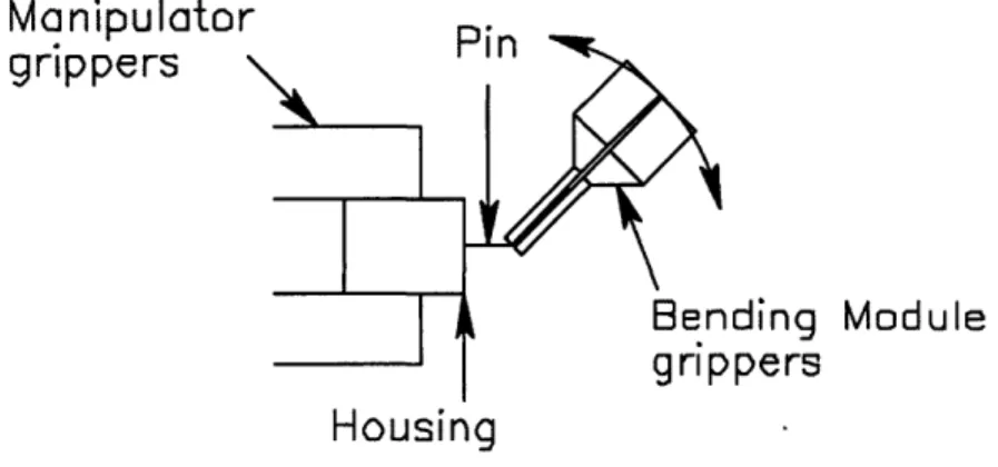
The parallel bending module can bend a parallel line of pins that have been previously inserted into the housing. It uses a pair of grippers that grab the line of pins, and then bends them with the axis of rotation being the desired location of the bend, as seen in figure 1.3.
MA
ni ulator
grippers
Iding
Module
>pers
Housing
Figure 1.3: Bending Module interfacing with the Manipulator on the Transport Module
The module as designed uses electrical conductivity between the pins and the grippers to measure the bend angle after elastic springback has occurred, and uses an adaptive algorithm to iteratively bend the row of pins until they have plastically deformed to the desired position, as in figure 1.4. It continues this algorithm until the angle measured is within some desired tolerance. This action, and the module, is discussed in detail elsewhere [3] and [4].
Start with POSdesired[O] = Desired Final Position
Bend to
Done
Figure 1.4: Iterative algorithm used for bending parts with the bending module. K is a constant less than
one.
The loader module presents an empty housing to the transport module, and the unloader removes the finished product from the transport module grippers. The design of each was intrinsically related to the that of the transport module, and hence, they are further
Chapter 2 Transport Module Design
The transport module must be able to accept an empty housing, take it to various
assembly stations, manipulate the housing in the ways required by those stations, and then drop off the finished product. It has been previously decided [2] that the transport module should contain all of the degrees of freedom common to the assembly modules' needs, so that the design would avoid using redundant axes at each assembly station. This simplifies the design of each of the assembly stations dramatically, and only complicates the
transport module somewhat.
The desired positioning capability of the entire system was required to be within 0.002 inches. To accommodate error in the assembly modules the transport module should be
able to position the housing within 0.0005 inches of the desired position. It should be able to move between assembly stations in a couple of seconds, as well as manipulate the housing dexterously enough to keep up with the assembly modules' speeds of operation.
The manipulator on the transport module should be able to position the housing along the X-, Y-, and Z-axes (as defined in figure 2.1), as well as rotations around the Y-axis. These are the degrees of freedom needed by the assembly modules. The transport module
follows the X-axis from one assembly station to another. The Y-axis is used to move the housing closer into the assembly module, and the Z-axis moves the housing up and down against gravity. Issues to be considered include:
* Actuation and position feedback for each needed axis, that is capable of the speeds and positioning required by each assembly station
* Actuators and structure that is capable of withstanding the forces of assembly * The manipulator's method for positioning / holding housing
r--- ·-
··-
Z
:)
It)·
-1 0
is
Figure 2.1: The axis orientation relative to a housing.
Section 2.1 Speed and Precision
First, consider the issue of actuation. The simplest possible system would to have be the four axes built on top of one another, as in Figure 2.2.
Figure 2.2: The simple 4-axis system showing definitions of axes
X- is
Y
Since the module would have to coordinate with several assembly stations, the estimated X-axis length is 10 feet. A linear encoder or some other long-range sensor, such as a laser interferometer, would have to be used to locate the module to the desired accuracy, as no actuator would be accurate enough with a rotary encoder over such long distances. If a leadscrew was to be used, then the pitch would have to be small in order to give the necessary resolution, but a small pitch corresponds to a proportional cut in speed, considering the critical speed of the screw (at which point the natural frequency of the screw is reached) and the thermal effects from friction at high screw speeds. Using a timing belt would involve problems such as flexibility in the belt when trying to perform small motions in the X-direction. In either case, the expense of a 10' linear encoder or a laser interferometer would be prohibitive. Other concerns would be the angular alignment along the linear guides in the X-direction, which would involve extensive error-mapping at each assembly station, and the lack of flexibility in changing the system around once it is set.
Section 2.1.1 Redundant X-axis
An alternative idea was dubbed the 'Redundant X-axis' system, as shown in figure 2.3. This would have a coarse and fine X-axis. The coarse X-axis would deliver the desired speed moving from station to station, while the fine X-axis would handle the small
motions and precise positioning. Some sort of docking mechanism would be necessary for the fine positioning table to be effective. Two kinds of docks were considered: a hard dock, which would force the manipulator into a desired position, at which point all locations are known to within the repeatability of the dock, and a soft dock, which would use sensors to measure the location of the manipulator, and then use the manipulator's axes to compensate for offsets in position.
The redundant X-axis system would be a step above the simple 4-axis system in that the coarse axis would have much more leeway in positioning the module, limited only by the
ability of the dock to compensate. The resolution of the coarse axis does not need the 0.0005" specifications, which eliminates the need for expensive sensors and equipment such as laser interferometers. Also, since the coarse axis does not need high resolution, and will only be moving the module comparatively long distances (at least a foot or so), using the redundant X-axis system opens up the choices for the coarse axis actuator, as
now both timing belts and leadscrews would no longer be troublesome, and other methods not considered before become available. For all of these reasons, the redundant X-axis system was chosen for the design.
Figure 2.3: The redundant X-axis system for coarse and fine motion
Section 2.1.2 Docking
Now to choose between the two basic docking methods mentioned above. The hard dock would be effective because it would position the module into a known and repeatable
position, at which point all commands would be the same. The transport module would have to have some play for the hard dock to be able to position it without damaging anything. The hard dock would have to be able to carry the weight of the entire
manipulator. The soft dock would involve several sensors, in each of X, Y, Z and angular directions. These would be placed on the module to avoid the redundancy of having the same sensors at each assembly station. However, the manipulator only needs to be 4 degrees-of-freedom (in order to give all the motions necessary for the assembly modules). and to compensate for other angular errors would either involve adding more axes, or to ignore a potential problem, as an angular error in the Z-direction could cause obvious problems in parallel bending or insertion, where the ends of a 4 inch housing would vary by 0.0012 inches for just a one arc-minute error. Hence, it was decided to pursue the hard docking idea more fully (see Section 3.2).
Section 2.2 Actuator and Structure Strength
The strength of the actuators and the transport module structure needed to be considered at this point. At the parallel insertion module, forces of up to 1000 lbs are needed to insert the row of pins at once. At the serial insertion, bending, and all other assembly stations strengths only a few pounds above that needed to move the transport module's weight itself are needed. In order to accommodate the parallel insertion, the Y-axis on the transport module would need to be able to provide 1000 pounds, and the structure would have to be able to withstand similar forces as well. This would yield a big, beefy transport module in order to accommodate just one assembly module. Thus, an 'assisted Y-axis' system was developed. The parallel insertion module would have its own Y-axis actuator which would be capable of delivering the 1000 pounds necessary for its operation. The transport module would 'hook in' to the assisting axis, which would then insert the pins. This would allow the transport module to be much smaller and more elegant than without this assisted system.
There were two choices as to the method of assistance, cleverly dubbed 'back push' and 'front pull'. Back push involves a rubber boot pushing at the back of the Y-axis carriage, or holding the Y-axis carriage in place while an actuator inserts the pins. This would mean that much of the structure would still need to support the heavy loads, although the transport module would not need to supply the actuation. Front pull has the manipulator grip the housing on the outside surface, leaving a gap between the housing and the manipulator body. At the parallel insertion station, it moves the housing in front of a backing, which is connected to the assisting axis. This way, the assisting axis is taking the entire load, allowing the structure of the transport module to be much lighter. This is shown in figure 2.4. Assisting Arm Assisting Arm 1 Trar Mod sing to Assisting
Axis
GrippersSide
Top
Figure 2.4: Front Pull Assisted Y-axis System
Section 2.3 Gripping and Locating
The manipulator could handle the housing in one of two basic ways:
* The manipulator grippers hold the housing using some sort of reference to position the housing repeatably.
* The manipulator grippers hold the housing more arbitrarily, and some sensing system locates the housing within the grippers, and uses this information to compensate.
The obvious solution for the first method is to incorporate some reference key into the grippers themselves. Each housing has a reference that can be used to locate the housing to within the tolerances of the housing itself. However, as each product may have a different reference, part-specific gripper fingers would be required. These could easily be
changed between runs if some locating method (such as location pins) is used. This appears to be capable if the reference is on the outside of the housing, but many times the reference is not, in which case this method becomes much trickier. Using the key to position the housing would require that the key withstand insertion forces as well.
Another possible solution would be to have the loading module present the housing exactly to the manipulator grippers, which would somehow conform to meet the presentation, but then stiffen to hold the housing in place. To do this would involve servos and multiple sensors on the manipulator grippers, which would be less than desirable.
The second 'compensation' method could be handled if the grippers could reasonably place the housing with negligible angular rotations in the directions that the manipulator is unable to compensate (that is, angular X and Z). A probe could be used to find the
reference on the housing, and relate that information back to the controller. However, it quickly became obvious that, since the locations of the holes in the housing were of critical importance, rather than the location of the reference (which is only used to estimate the location of the holes), the sensor could be used to locate the holes directly. This would eliminate the tolerances between the reference and the holes by finding the holes
themselves.
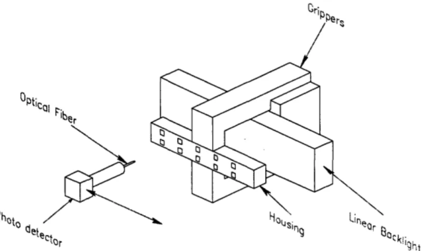
Hole detection quickly turned to optics. At the loading module the manipulator can move the housing over a backlight, much like it moves over the assisting Y-axis at the parallel
insertion module. An optical fiber can then be scanned across the surface of the housing, as in figure 2.5, below. Regions of light and darkness can then be read by a
photodetector, and this information can be used to estimate the locations of the holes in the housing. The optical fiber would not be able to detect distance or X and Z angular errors, however, so the grippers would have to hold the housing to suppress errors in those directions, and once the location was found, the housing could not slip in the grippers without potentially catastrophic results.
Okti'-.
Figure 2.5: Shows the backlight and the photodetector, both of which are connected to the loading
module, while the grippers are attached to the transport module.
A video camera could also be used to snap a picture of the backlit housing, and this information could be analyzed by a computer to estimate the hole locations. This would be more expensive than the optical fiber method, as well as bulkier. Also, the optical fiber could almost enter the holes themselves, whereas the camera would have to be a few inches back from the detector. Thus the camera would be more likely to be effected by possible diffraction effects in smaller housings. The software would be more demanding, and it would take longer to program for a new product.
The optical fiber hole detection was the most novel, simple, inexpensive, and flexible option found for locating and gripping the housing, and was chosen for this system. More on this method is detailed later (Chapter 6) and elsewhere [4].
-"o ,
Phot .
The grippers have to be able to position the housing with negligible error in the Y-direction as well as the Z and X angular Y-directions. A 'universal' gripper can properly hold a class of housings: those that are rectangular in shape, do not have surface features
along the face of the long sides, and have a 'lip' at the front edge (see figure 2.6). Although this may appear to limit the flexibility greatly, a significant percent of products fit this description. Most others can be properly held using part-specific grippers. In order to facilitate changing grippers for different parts, and to keep expenses and new product time down, only the gripper 'fingernails' are part specific, and can be changed rapidly and repeatably using location pins.
FJIl Svurfce
I Li
Interchdngedble Grippe r
Fingernrils
Figure 2.6: Shows gripper holding 'universal' housing with 'universal' fingernails
The grippers and fingernails themselves are precisely made within the angular tolerances needed. The housing pressed between these surfaces should be reasonably well protected against X-axis angular errors, which is not a sensitive direction anyway. The loading module pushes the housing into the grippers until the alignment lip presses against the gripper fingernails. This should eliminate most Z-axis angular errors, and should
reasonably position the housing in the Y-direction. When the grippers are held tight, the housing should not move. If both the housing and fingernail surface are very hard, then surface imperfections can cause the housing to be held at only the highest surface, which
may cause the housing to swing. The alignment lip should handle this problem in most cases, but a very thin flexible layer (a few thousandths of an inch) can be applied to the fingernail surface if this is seen and the alignment lip is either ineffective or, for some reason particular to the product, not present.
Chapter 3 Transport Module Details
Now that the basic foundations of the transport module were designed, the details could be ironed out. Still to be considered include:
* Choice of manipulator axis orientation * Design of hard dock
* Choice of coarse X-axis actuator
* Choice of manipulator actuators (types, motors, etc.)
Section 3.1 Axis Orientation
One possible manipulator orientation is shown previously in Figure 2.3. The Z-axis lies on the Y, which lies on the fine X-axis. The rotary axis is attached to the Z, and the
manipulator grippers are attached to the rotary. In order to get the full range of motion required by the assembly modules, each linear axis needs a range of 6 inches, and the rotary axis needs to be able to rotate 1800.
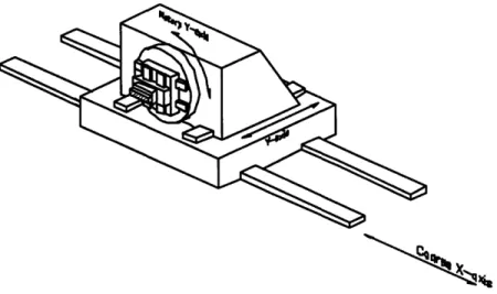
Another possible axis orientation was dubbed the 'rotating X and Z'. These mount the fine X and Z on the rotary axis as shown in Figure 3.1, below.
Figure 3.1: The 'rotating X and Z' system with fine axes on the rotary table
For the ranges of motion required by the assembly modules this system requires that the fine X- and Y-axes each have a range of 6 inches, and the fine Z- has a range of 2 inches. The change from above is that now the X and Z-axes can essentially be switched by turning the rotary table. This would have advantages in ease of use if diagonal motions were required. However, during assembly operations the rotary axis will only be making 900 turns, so this apparent advantage is negated. Also, this would require more weight hanging cantilever-like off the rotary table, as well as requiring small X and Z tables that can take the necessary loads.
Because of these complications, the original 'intuitive' orientation was chosen over the 'rotating X and Z'. This allows for basically identical, somewhat beefy, X-, Y-, and Z-axes.
Section 3.2 Docking
For reasons cited earlier it was decided to go with a hard-docking scheme. In order for the manipulator to interface properly with the assembly modules, the entire manipulator (consisting of the X-, Y-, Z-, and rotary Y-axes, as well as the grippers) must be docked properly. The repeatability of the docking plus the repeatability of the fiber locator plus
the resolution of the servo tables making up the manipulator must all add to less than the desired positioning ability of 0.0005 inches. Leaving reasonable values for the servo resolution and fiber location ability, the dock should be repeatable to about 0.00025 inches. The manipulator should also be able to quickly and easily dock, as this shouldn't need to be a complicated operation with multiple motors and such.
The transport module would move over to the dock, at which point the manipulator would mate with the assembly module, and somehow detach from the transport module (or some other method of removing the constraints of the transport module on the manipulator).
A Manipulator
D)
Coar
Docking Base
Figure 3.2: The coarse X-axis carriage moves the manipulator over the docking plate attached to the assembly module, as in A. It then sets the manipulator down upon that docking plate, so that the manipulator is in contact with the assembly module alone, as in B.
Many common docks, or couplings, use a large contact area to average out surface inconsistencies in order to dock repeatably. This is called elastic averaging. The dock's repeatability, disregarding thermal effects or dirt contamination, will be on the order of the
precision of the manufacturing of the mating faces of the dock [5]. However, thermal effects (if any) or dirt contamination must be avoided. Since area of contact is large, surface contact stresses tend to be low, and the coupling can handle high loads.
Another coupling is the kinematic coupling. One face has 3 v-grooves machined into it, and the opposite face has 3 balls that are set into the opposing grooves (see figure 3.3). As the contact area of the balls on the grooves is small, they can be estimated as point contacts. Three balls in 3 grooves gives exactly 6 points of contact, which constrain exactly 6 degrees of freedom. Unlike elastic averaged couplings (which are
overconstrained), kinematic couplings are completely deterministic, which allows one to calculate deformations and positions through the coupling. However, since the contact areas are small, surface contact stresses are high, limiting the amount of load the coupling can carry.
The kinematic coupling works so well because it is made while mated. The balls (or cones, or some other shape) are attached (by epoxy, for instance) to their plate while the coupling is mated in its final location, with real working loads applied. The fit is almost exact because it was made to be so. This also makes the machining precision less demanding. On account of the way the mating faces are made, the repeatability can be extremely good, on the order of a microinch [5].
On the assembly line, the groove face would be attached to the manipulator, and each assembly station would have a ball face of the coupling set to the groove face on the manipulator.
The groove can be a separate piece machined in a curved shape (a gothic arch, for instance) to give a greater equivalent radius between the ball and groove surface, which increases the load bearing capability of the coupling. A calculation of the Hertz contact stress [5] of the interface will determine what radii to use:
1 1 3E__F
q
-
,
)"(
2
eqn 3.1
where q is the contact stress at the center of the contact area, Re is the equivalent sphere on flat plate radius of the ball and groove interface, Ee is the equivalent young's modulus of the two materials used for the ball and groove, and F is the load at the interface. The
1
equivalent radius is Re
1
1
1
1
eqn 3.2
where R1 and R2 are the radii of the ball and groove, respectively, and the equivalent
1
Young's Modulus is E, = eqn 3.3
+
-E1 E2
where rTl, r72, El, and E2 are the Poisson's ratios and Young's moduli for the ball and groove, respectively.
For metals, a conservative estimate for the maximum Hertzian contact stress is given as follows [5]:
3c"
qmax = max eqn 3.4
2
where o,,,,, is the maximum allowable tensile stress in the metal.
The coupling preload should be about the same each time the manipulator is mated with the assembly stations. For greatest stability, and to allow for a larger coupling, the manipulator should rest on the coupling, rather than, say, a vertical coupling, which has several obvious disadvantages and complications (cantilever, high moments on the
coupling, etc.). The preload on the coupling then includes the manipulator's own weight. with the addition of a 100 lb. clamping force (for greater stability, accuracy, and ease of mind).
Judging by the estimated size of the manipulator (considering the approximate size and weights of servo tables), the coupling needn't be small, and using a spreadsheet that related forces and moments from the housing to the balls, it was estimated that 1 inch radius balls (given a factor of safety of two) would be adequate, placed at a radius of 5.5 inches. The wide base (11 inches diameter) was necessary to ensure that none of the balls would lift off during insertion operations. As the bulk of the parallel insertion forces would be handled by the assembly module (see assisted Y-axis design, section 2.2),
without which this all would not be feasible, the loads and deflections were calculated for various extremes of manipulator position, and for estimated assembly loads. The serial
insertion was estimated at 25 lbs, and the parallel bending was liberally approximated at 10 lb in. Details of the calculations and parameters are given in Appendix B.
The deflection at each of the contact points can be calculated using the following formula
[5]
1 3F 3
I= 1eqn 3.5
2 Re 2
)
where 6 is the elastic deflection at that point. Using equation 3.5, it was possible to calculate the changes in deflection with different manipulator positions and assembly operations, and relate that back to the deflections at the toolpoint. The total deflection at the toolpoint for serial insertion was calculated to be 0.00026", and was 0.0000086" for bending, which meets specifications fairly well.
Since the kinematic coupling was capable of meeting the docking needs, is less expensive than the precise machining needed for an elastic averaged coupling to meet the
performance requirements, and far more repeatable than those couplings, it was chosen for use in this design.
The application of the 100 lb. clamping force preload to the coupling had yet to be
specified. The connection between the coupling plates was desired to be 6 points (in order to utilize the capability of the kinematic coupling to its maximum), the clamping force would have to be entirely down, that is, to work to put the plates together with no transverse forces. Several complicated ideas were brought up involving intricate
mechanisms in which the plates would grab each other. Each would involve a significant amount of hardware design, and it was questioned as to whether they would actually work as desired.
A electromagnetic clamp, mounted in the base coupling, and 'attracting' the iron coupling plate attached to the manipulator, would truly exert no other forces but for the desired
direction, as the clamp would not need to involve contact. As magnetic fields disperse quickly in air (as the cube of the distance), the gap between the plates must be kept very small, and was chosen to be 0.010". Further discussion and explanation of the choices involved pertaining to this issue are presented elsewhere [4].
ectromogYne
y
wfViA7tfl
Figure 3.4: This is the lower plate of the kinematic coupling with the electromagnet installed in the center. The electromagnet bonds with the steel disc of the upper coupling plate.
Potential problems with using the magnetic coupling include the extensive magnetic fields involved and the potential for contamination. However, since magnetic fields disperse as the cube of the distance, they were not seen to be a serious problem. Contamination of size larger that the gap (0.010") could cause the coupling to rest improperly. The magnetic clamp would not be on while the mating coupling is not present, which suppresses the imagined problem of little metal pieces flying across the room to stick to the clamp, despite the fact that the metal disc of the manipulator's coupling is necessary to complete the magnetic field's 'circuit'. The transport module could carry a brush at its
front that will brush off the base as it passes over if contamination is seen to cause problems.
A magnetic clamp was designed, built, and tested by Oei [4] that would fit into the present system design without any major modifications.
Section 3.3 Transport
The redundant X-axis system (see Section 2.1, above) opens up just about anything for use as the coarse X-axis. The coarse X-axis actuator should be able to move the transport module between assembly modules in a few seconds or less, and should be able to position the manipulator within 1/4" of the desired location, so that the kinematic coupling will match up well enough to settle properly with the balls in the grooves. Several methods were analyzed, beginning with the leadscrew.
A screw with a large pitch would be able to move the module quickly, and position it well enough for the coupling to do the rest without any expensive sensors such as laser
interferometry.
A belt drive, depending on motor choice, could also deliver the required speed and location ability. The module could ride on plain rails, as precise bearing rails would be unnecessary.
The module could also be an automated guided vehicle (AGV) on wheels. Motors could be built into the module, which drive the wheels directly. Some steering mechanism would also be required. The module would then follow directions using sensors, such as following some feature on the floor from station to station. Often this is as simple as following a strip of tape, paint, or electric wire using various sensors. Automated guided vehicles and the technology for them are well documented and proven.
The automated cart would have to receive a signal that commands it when to stop. This can be from some breakbeam sensors near the assembly module, or perhaps an inductive sensor on the cart that can sense the electromagnet assembly below it. The cart would use a tether of cables for power and command.
Guided vehicles have been shown to be able to deliver the 1/4" precision in location needed to place the kinematic coupling faces so that they can mate [6]. If more precision is desired (for piece of mind perhaps), the cart could easily drive into guides that tightly control the module's direction as it approaches the assembly module, much like how car rides in amusement parks do not allow the car to leave the path.
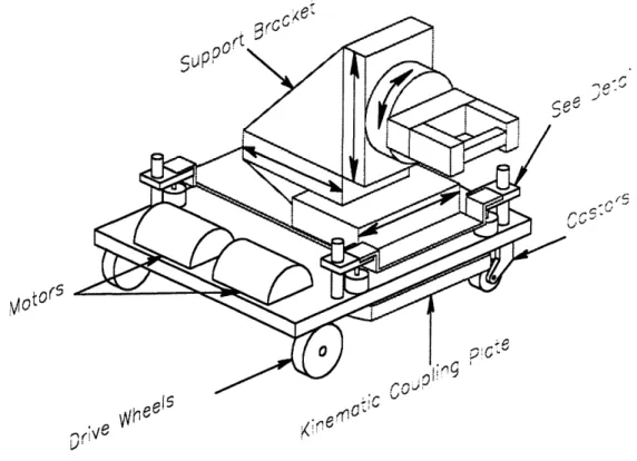
In essence, the transport module could be seen as a car elevated in a repair body shop. It approaches an assembly module so that the coupling faces are close enough that they can mate, and then the manipulator either drops out of the cart, or 'rover', onto the coupling below, or the coupling below can lift the entire transport module, so that the only contact between the module and the ground occur through the coupling (lifting it off its wheels. so to speak). When the assembly operations are complete at that module, the cart is set down and drives off to the next assembly module.
The automated cart, or 'rover', is the most flexible option, as the line can easily be changed by just changing the tape on the floor. The screw and belt drives all require significant modifications when changing the length or set up of the assembly line. The line is also no longer required to be linear in set up, and time can be saved by having the transport module traverse a circle on the floor (although the tether may have to be reconsidered, which is a complication that won't be discussed, but this is an example of how the design allows the flexibility for improvement through future work, whereas the other designs do not). The cart also leaves the most play for coupling location, being that it is not attached to a screw, belt, or on rails, and it does not require bulky equipment on the line or extensive set up costs. This is also the most novel approach of the three
methods described above. For these reasons, the design moved to that of an independent manipulator resting upon an independent rover, the results of which can be seen in Chapter 4.
Section 3.4 Rover Design
Some details of the rover design had yet to be worked out: * the method of steering the rover
* the method of guiding the rover
* the type of coupling actuation (i.e., the 'elevator') by which the manipulator docks and undocks.
* the method of commanding the rover to stop
* safety issues
There are several possible methods for steering the rover. Differential steering uses two wheels powered separately. When powered at different rates, the cart will turn, much in the same way as a military tank. Castors would then be added to round out the support for the cart. Otherwise, only one motor is used and some steering mechanism must be developed to turn the wheels. Optionally, the cart could follow a rail rather than have any steering at all. This last method would lose some of the flexibility advantages of the AGV, but would make for a simple set-up for a prototype design. Differential steering does not involve designing a steering mechanism, which makes it simpler to design and build, and so was chosen for the final design.
There are two common methods for vehicle guidance: optical path following and wire following.
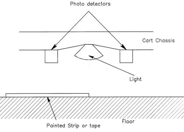
Using a pair of optical sensors on the underside of the transport module that are either on or off depending on the darkness of the floor beneath, the module would be able to follow
a lightly colored tape across a dark floor, or vice versa, along as there is reasonable
contrast between the line and the floor (see Figure 3.5). If the light following sensor drifts off the tape, and the other does not drift onto the tape, then a microprocessor in the cart knows to which side that it has drifted off the path. The path could be easily altered by removing and re-applying tape. The disadvantage of optical following is that dirt build-up on the floor can cause loss of signal. But if the assembly line is being reconfigured
regularly (with a new path being laid), then this should be less of a problem.
Photo detectors
Chassis
Light
Floor
Painted Strip or tape
Figure 3.5: Optical guidance method showing underside of front of cart
More commonly in industry, a pair of inductive sensors follow a electric wire imbedded in the floor [6]. If the cart drifts from the path so that one sensor picks up a greater signal than the other, the steering mechanism compensates the vehicle until the sensors' signals are again equal. It is generally accepted that wire guidance gives better tracking than
optical guidance, but rearranging the assembly line would be more complicated. Taping the wire down, rather than actually imbedding it in the floor can alleviate this
disadvantage, but then the operators must take certain steps to ensure that the wire does not present a danger to any employees (i.e. tripping).
There are several other methods of vehicle guidance, including inertial guidance,
triangulation, and optical or ultrasonic imaging. None of these methods are as widely used as optical or wire guidance, and none of the technologies are as fully developed or as proven as the two previously discussed [6].
Because of previous experience with optical following, this method was chosen for this design. However, the advantages of wire guidance must be kept in mind, and switching from optical to wire guidance is straightforward and can be done at any time.
An elevator system needed to be developed to dock and undock the manipulator with the assembly module. This could be built into either the floor or the transport module. It requires a range of motion of one inch, and should be able to lift about 60 lbs.
A simple idea involves the wheels of the rover rolling into 1" deep dips, at which point the coupling will be aligned well enough that the manipulator will couple as required. The rover and manipulator would be two separate pieces, with the rover (with a coupling-sized hole in the middle) supporting the manipulator by 'wings'. When the rover sinks down into the recesses at the base of the assembly module, the manipulator will be left resting on the coupling (see Figure 3.6). When assembly is done, the rover will drive out of the dips, picking up the manipulator on the way. There are several problems with this approach,
however. It would be difficult to rest assured that the manipulator's coupling half is going to mate properly with that of the base, being that everything is moving laterally as well as up and down. The kinematic coupling isn't tremendously resistant to shocks, and the mating process (involving free falling) wouldn't be without shock. Also, having the rover
drive out of the holes would require more traction and power than would be needed otherwise.
Manipulator
Rover Coupling Base
Figure 3.6: The cart carries the manipulator by the winged flange. When the cart is in the holes and the manipulator is docked, the rover and manipulator are no longer in contact.
Another option is to use the same configuration with the rover and cart, but use a pneumatic lift in the coupling base rather than the 'crude' dips. The lift would raise the manipulator off of the rover once the rover has stopped over the coupling, giving more piece of mind as to the locating ability of the coarse X-axis system than the previous idea (see figure 3.7). As the designer would have control over the speed of the lift (using dampers or what-not), impact can be kept to a reasonable level. This design is dependent upon the lift's locational repeatability (end point of stroke, as well as play transverse to the stroke), however, and the docking precision requirement would likely no longer be met.
Manipulator
Rover
Coupling Base
Figure 3.7: The cart carries the manipulator by the winged flange. When the lift extends, it raises the manipulator off the rover so that the manipulator and rover are no longer in contact.
Rather than using the lift to raise the manipulator, use the lift to lower the rover. The manipulator will lower with it until it comes in contact with the coupling base, which is rigidly attached to the assembly module. The positioning capability of the coupling is not being compromised by the lift. This would require each assembly module to have a lift, and requires mechanisms to be built into the floor, or to have the rover traverse a ramp.
Lastly, the rover can carry a pneumatic lift, which lowers the manipulator onto the base when the rover stops at the assembly module. When assembly is complete at that module, the lift picks up the manipulator and carries it off. Building the lift on the rover eliminates the need to have a lift at each assembly module, although it requires that the tether have pneumatic tubes. It also assures a rigid connection between the manipulator and the assembly module, and takes full advantage of the kinematic coupling's repeatability. Because of the lack of redundancy offered by having the lift on the rover, and the availability of pneumatic cylinders of the size and stroke length needed, it was chosen to have the lift on the rover rather than in the base.
As the rover approaches the assembly module, it must receive some signal to stop. An easy method for this could be to use three breakbeam sensors in the vicinity of the
assembly module: when the rover triggers the first it begins to slow down, and then aligns itself so that it lies between the final two, so that any deviation greater than that needed for the coupling would trigger one beam. Other methods were discussed, including using an inductive sensor to detect the electromagnet (on low power) as the cart passed over the coupling. As the direction of the research was soon to take a turn, and because this was not an issue of critical importance or ground-breaking excitement, this issue was never fully decided.
There are several safety issues that need to be addressed when using AGV's. Bumpers. both hard (for contact) and soft (a proximity sensor that can command the cart to slow before contact occurs), should be installed. The cart must also be programmed to stop if
it loses contact with its path. These issues were never fully addressed, as there exist safety standards in industry for AGV's [6].
Chapter 4 The Final Design
The final transport module design consists of two parts: a 4-axis manipulator that securely grips a housing located using the fiber-optic method described above (section 2.3) and detailed below (see chapter 6), and a guided rover that moves the manipulator from one
assembly module to another. Upon reaching an assembly module, the manipulator is set down upon the highly repeatable kinematic coupling, separating it from the rover. At this point the manipulator has essentially become part of the assembly module. An
electromagnet is used to securely clamp the manipulator down. When the operations are complete at that module, the clamp turns off, the rover lifts the manipulator off of the coupling and drives off, optically following a line of tape to the next assembly module.
-"n-CrC
rr
VotorsvV,,e"
,rJe , ,;vl ":Figure 4.1: A sketch of the manipulator and rover of the final design. The manipulator is light lined. Arrows show servo axes.
Manipu I ator
Guide post
P n e U
Wf'i_..y
Figure 4.2: Transport Module Detail. The pneumatic cylinder raises and lowers the manipulator, which rests on the plate. The guide post gives the cylinder support against transverse forces.
Rather than build a steering mechanism, the rover drives each of the main wheels separately. Driving the wheels at different rates will cause the cart to turn, much like a military tank. The other side of the cart is supported by castors.
The front of the cart has two light sensors. One looks for light, the other for dark, so that the cart steers to follow the tape edge. There are several viable options for warning the cart when and where to stop, and this issue remains to be fully configured.
Four pneumatic cylinders act in concert to raise and lower the manipulator on and off the mating face of the coupling beneath the cart. The cylinders are set up to push up on supports attached to the manipulator. The range of motion of the lifts is greater than that needed to lower the manipulator onto the coupling base, so that the cylinders, and the entire rover, are no longer in contact with the manipulator when it is docked.
Each assembly module is rigidly attached to a kinematic coupling, whose balls are set to mate exactly with the 'groove' side underneath the manipulator, which rests on the coupling when performing assembly operations. An electromagnet is mounted in each coupling base. This clamps the manipulator down by attracting the manipulator's steel coupling plate.
The manipulator consists of three 6" linear stages and one rotary stage, each easily chosen from common stock items. The gripper is attached to the rotary stage. The gripper holds the housing by means of detachable 'fingernails', which are designed to align the part in the angular Z-direction, angular X-direction, and the Y-direction. A fiber-optical locating system is used to measure the X and Z location of the housing by measuring the locations of the holes themselves, and the housing is held firmly in this location throughout its assembly.
Section 4.1 The Experimental Testbed
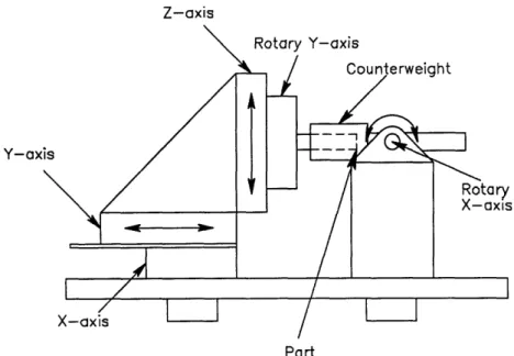
A multi-functional experimental testbed was built for testing some of the ideas of the transport module design, such as the optical hole-finding technique. This testbed consists of the manipulator design for the transport module rigidly bolted to the baseplate of the bending module previously built (see figure 4.3). This gives a 5-degree of freedom system with linear X, Y, and Z, and angular Y on the manipulator, and angular X on the bender.
Z-axis
Y-ax
Part Figure 4.3: Schematic of the Experimental Testbed.
Figure 4.4: The experimental testbed consisting of the manipulator and rotary bender designed for assembly line.
The manipulator portion of the testbed was designed to be used as the manipulator on the transport module if the assembly line is built in the future. The manipulator is built of three 6" linear leadscrew stages and one worm-driven rotary stage, all purchased from stock components from Daedal (part #'s 106061P and 20602-P). All were chosen to withstand the force and moment requirements found for each using a spreadsheet that calculates forces and moments from the tool-tip to the base, using the weights and joint displacements between each component, as well as forces on the tool-tip (see Appendix B).
The leadscrews each have a 5 pitch, which allows for a speed of 3 inches per second at the maximum rate of the screw, and with 4000 count rotary encoders (quadrature) gives 20000 counts per inch, or 0.00005". The motor torque required to accelerate the load, the screw, and to overcome screw friction with a maximum linear acceleration of 12 in/sec2 needs a motor torque of 6.93, 12.00, and 18.81 oz inches for the Z-, Y-, and X-axes, respectively (they increase because of the increasing load on each).
The rotary table was chosen to have a resolution of 0.06 arcminutes (a worm gear ratio of 90 with a 4000 count encoder), which gives a 0.00005" Abbe error at 3" from the table center-line. Since mostly the table will be used to orient the housing between assembly stations, and not during assembly operations, a modest velocity of .167 rev/sec was adequate. A torque of 20.04 oz inches was required for an acceleration of 1 rev/sec. Since the motor demands for all of the tables were similar, the same motor was chosen for each, a 70 oz inch stock motor, the 7ME70H from Motion Science (more torque than necessary, but they were readily available with only a modest cost and weight increase over the 35 oz inch version). These were powered by Motion Science amplifiers, part number DHB5006HX.
Gripper Design
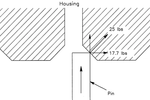
The gripper will use the housing's lip for resisting insertion forces in the Y-direction, or if the housing doesn't have a lip, part-specific fingernails will be used that have a lip for a backstop. So the gripper only needs to grip securely enough to resist transverse forces.
Since the holes are chamfered, for ease of insertion, the transverse forces were
approximated as if the inserter pushed the pin into the chamfer, that is, the 25 lb. insertion force hits at an angle of 450, causing a transverse force of 17.7 lbs, as shown in figure 4.5.
below.
Housing
Figure 4.5: Transverse force caused by misaligned pin hitting chamfer used for calculating necessary gripper strength.
Guessing at a coefficient of friction between the gripper fingernail and the housing to be 0.2 (fairly arbitrary, but conservative), the needed gripper force for the housing not to slip in the grippers during insertion is 88.5 lbs. A pneumatically-actuated gripper was chosen from stock that can deliver 121 lbs with a pressure of 6 bars, has a stroke length of 0. 16"
admissible forces of 135 lbs and 3800 oz inches, and weighs just 1 lb (the Schunk PGN
80).
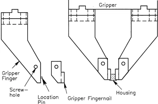
The grippers and gripper fingernails were made of steel, for strength. They were made angled (see figure 4.6, below) in order for the rotating grippers on the bender to be able to rotate up to 1200. A pair of location pins are used to position the fingernails on the
fingers, which are then screwed down. The fingers are also positioned on the grippers using pins. The surface of the fingernails have been machined to a 0.0005" flatness.
ho e - -• Housing
Location Gripper Fingernail Pin
Figure 4.6: Showing the design of the gripper fingers and fingernails.
The bending module was increased in height in order to correspond to that of the
manipulator. It was also modified to have a toolbar with regularly placed screw-holes so that other tools can easily be attached to the bender axis, other than just the rotating grippers of the original design.
Figure 4.7: The grippers, mounted on the rotary axis on the manipulator, interfacing with the rotary bender.
The system was controlled by Tech-80 5650 and 5650A motion control-boards in a Compaq Prolinea 575 PC with a 75 MHz Pentium Processor. With the addition of a National Instruments AT-MIO XE-50 data-acquisition board, the experimental testbed became a flexible, accurate, and automated experimental laboratory that would form the base for the experiments dealing with fiber-optic hole location and coplanarity detection and compensation.