Monte-Carlo Tree Search by Best Arm Identification

HAL Id: hal-01535907

https://hal.archives-ouvertes.fr/hal-01535907v2

Submitted on 5 Nov 2017

HAL is a multi-disciplinary open access

archive for the deposit and dissemination of

sci-entific research documents, whether they are

pub-lished or not. The documents may come from

teaching and research institutions in France or

abroad, or from public or private research centers.

L’archive ouverte pluridisciplinaire HAL, est

destinée au dépôt et à la diffusion de documents

scientifiques de niveau recherche, publiés ou non,

émanant des établissements d’enseignement et de

recherche français ou étrangers, des laboratoires

publics ou privés.

Monte-Carlo Tree Search by Best Arm Identification

Emilie Kaufmann, Wouter Koolen

To cite this version:

Emilie Kaufmann, Wouter Koolen. Monte-Carlo Tree Search by Best Arm Identification. NIPS 2017

- 31st Annual Conference on Neural Information Processing Systems, Dec 2017, Long Beach, United

States. pp.1-23. �hal-01535907v2�

Monte-Carlo Tree Search by Best Arm Identification

Emilie Kaufmann

_{and Wouter M.Koolen}

1

_{CNRS & Univ. Lille, UMR 9189 (CRIStAL), Inria SequeL, Lille, France}

2

_{Centrum Wiskunde & Informatica, Science Park 123, 1098 XG Amsterdam, The Netherlands}

Abstract

Recent advances in bandit tools and techniques for sequential learning are steadily enabling new applications and are promising the resolution of a range of challenging related problems. We study the game tree search problem, where the goal is to quickly identify the optimal move in a given game tree by sequentially sampling its stochastic payoffs. We develop new algorithms for trees of arbitrary depth, that operate by summarizing all deeper levels of the tree into confidence intervals at depth one, and applying a best arm identification procedure at the root. We prove new sample complexity guarantees with a refined dependence on the problem instance. We show experimentally that our algorithms outperform existing elimination-based algorithms and match previous special-purpose methods for depth-two trees.

1

Introduction

We consider two-player zero-sum turn-based interactions, in which the sequence of possible successive moves is represented by a maximin game treeT . This tree models the possible actions sequences by a collection of MAX nodes, that correspond to states in the game in which player A should take action, MIN nodes, for states in the game in which player B should take action, and leaves which specify the payoff for player A. The goal is to determine the best action at the root for player A. For deterministic payoffs this search problem is primarily algorithmic, with several powerful pruning strategies available [20]. We look at problems with stochastic payoffs, which in addition present a major statistical challenge.

Sequential identification questions in game trees with stochastic payoffs arise naturally as robust versions of bandit problems. They are also a core component of Monte Carlo tree search (MCTS) approaches for solving intractably large deterministic tree search problems, where an entire sub-tree is represented by a stochastic leaf in which randomized play-out and/or evaluations are performed [4]. A play-out consists in finishing the game with some simple, typically random, policy and observing the outcome for player A.

For example, MCTS is used within the AlphaGo system [21], and the evaluation of a leaf position combines supervised learning and (smart) play-outs. While MCTS algorithms for Go have now reached expert human level, such algorithms remain very costly, in that many (expensive) leaf evaluations or play-outs are necessary to output the next action to be taken by the player. In this paper, we focus on the sample complexity of Monte-Carlo Tree Search methods, about which very little is known. For this purpose, we work under a simplified model for MCTS already studied by [22], and that generalizes the depth-two framework of [10].

1.1

A simple model for Monte-Carlo Tree Search

We start by fixing a game treeT , in which the root is a MAX node. Letting L be the set of leaves of this tree, for each ℓ∈ L we introduce a stochastic oracle Oℓthat represents the leaf evaluation or play-out performed when this leaf is reached by an MCTS algorithm. In this model, we do not try to optimize the evaluation or play-out strategy, but we rather assume that the oracleOℓproduces i.i.d. samples from an unknown distribution whose mean µℓis the value of the position ℓ. To ease the presentation, we focus on binary oracles (indicating the win or loss of a play-out), in which the oracleOℓis a Bernoulli distribution with unknown mean µℓ(the probability of player A

winning the game in the corresponding state). Our algorithms can be used without modification in case the oracle is a distribution bounded in[0,1].

For each node s in the tree, we denote byC(s) the set of its children and by P(s) its parent. The root is denoted by s0. The value (for player A) of any node s is recursively defined by Vℓ= µℓif ℓ∈ L and

Vs= { maxc∈C(s)Vc if s is a MAX node, minc∈C(s)Vc if s is a MIN node. The best move is the action at the root with highest value,

s∗= argmax s∈C(s0)

Vs.

To identify s∗(or an ǫ-close move), an MCTS algorithm sequentially selects paths in the game tree and calls the corresponding leaf oracle. At round t, a leaf Lt∈ L is chosen by this adaptive sampling rule, after which a sample Xt∼ OLtis collected. We consider here the same PAC learning framework as [22,10], in which the strategy also requires a stopping rule, after which leaves are no longer evaluated, and a recommendation rule that outputs upon stopping a guess ˆsτ∈ C(s0) for the best move of player A.

Given a risk level δ and some accuracy parameter ǫ≥ 0 our goal is have a recommendation ˆsτ∈ C(s0) whose value is within ǫ of the value of the best move, with probability larger than 1− δ, that is

P(V (s0) − V (ˆsτ) ≤ ǫ) ≥ 1 − δ.

An algorithm satisfying this property is called(ǫ,δ)-correct. The main challenge is to design (ǫ,δ)-correct algo-rithms that use as few leaf evaluationsτ as possible.

Related work The model we introduce for Monte-Carlo Tree Search is very reminiscent of a stochastic bandit model. In those, an agent repeatedly selects one out of several probability distributions, called arms, and draws a sample from the chosen distribution. Bandits models have been studied since the 1930s [23], mostly with a focus on regret minimization, where the agent aims to maximize the sum of the samples collected, which are viewed as rewards [18]. In the context of MCTS, a sample corresponds to a win or a loss in one play-out, and maximizing the number of successful play-outs (that correspond to simulated games) may be at odds with identifying quickly the next best action to take at the root. In that, our best action identification problem is closer to a so-called Best Arm Identification(BAI) problem.

The goal in the standard BAI problem is to find quickly and accurately the arm with highest mean. The BAI problem in the fixed-confidence setting [7] is the special case of our simple model for a tree of depth one. For deeper trees, rather than finding the best arm (i.e. leaf), we are interested in finding the best action at the root. As the best root action is a function of the means of all leaves, this is a more structured problem.

Bandit algorithms, and more recently BAI algorithms have been successfully adapted to tree search. Building on the UCB algorithm [2], a regret minimizing algorithm, variants of the UCT algorithm [17] have been used for MCTS in growing trees, leading to successful AIs for games. However, there are only very weak theoretical guarantees for UCT. Moreover, observing that maximizing the number of successful play-outs is not the target, recent work rather tried to leverage tools from the BAI literature. In [19,6] Sequential Halving [14] is used for exploring game trees. The latter algorithm is a state-of-the-art algorithm for the fixed-budget BAI problem [1], in which the goal is to identify the best arm with the smallest probability of error based on a given budget of draws. The proposed SHOT (Sequential Halving applied tO Trees) algorithm [6] is compared empirically to the UCT approach of [17], showing improvements in some cases. A hybrid approach mixing SHOT and UCT is also studied [19], still without sample complexity guarantees.

In the fixed-confidence setting, [22] develop the first sample complexity guarantees in the model we consider. The proposed algorithm, FindTopWinner is based on uniform sampling and eliminations, an approach that may be related to the Successive Eliminations algorithm [7] for fixed-confidence BAI in bandit models. FindTopWinner proceeds in rounds, in which the leaves that have not been eliminated are sampled repeatedly until the precision of their estimates doubled. Then the tree is pruned of every node whose estimated value differs significantly

from the estimated value of its parent, which leads to the possible elimination of several leaves. For depth-two trees, [10] propose an elimination procedure that is not round-based. In this simpler setting, an algorithm that exploits confidence intervals is also developed, inspired by the LUCB algorithm for fixed-confidence BAI [13]. Some variants of the proposed M-LUCB algorithm appear to perform better in simulations than elimination based algorithms. We now investigate this trend further in deeper trees, both in theory and in practice.

Our Contribution. In this paper, we propose a generic architecture, called BAI-MCTS, that builds on a Best Arm Identification (BAI) algorithm and on confidence intervals on the node values in order to solve the best action identification problem in a tree of arbitrary depth. In particular, we study two specific instances, UGapE-MCTS and LUCB-MCTS, that rely on confidence-based BAI algorithms [8,13]. We prove that these are (ǫ, δ)-correct and give a high-probability upper bound on their sample complexity. Both our theoretical and empirical results improve over the elimination-based state-of-the-art algorithm, FindTopWinner [22].

2

BAI-MCTS algorithms

We present a generic class of algorithms, called BAI-MCTS, that combines a BAI algorithm with an exploration of the tree based on confidence intervals on the node values. Before introducing the algorithm and two partic-ular instances, we first explain how to build such confidence intervals, and also introduce the central notion of representative childand representative leaf.

2.1

Confidence intervals and representative nodes

For each leaf ℓ∈ L, using the past observations from this leaf we may build a confidence interval Iℓ(t) = [Lℓ(t),Uℓ(t)],

where Uℓ(t) (resp. Lℓ(t)) is an Upper Confidence Bound (resp. a Lower Confidence Bound) on the value V (ℓ) = µℓ. The specific confidence interval we shall use will be discussed later.

These confidence intervals are then propagated upwards in the tree using the following construction. For each internal node s, we recursively defineIs(t) = [Ls(t),Us(t)] with

Ls(t) = { maxc∈C(s)Lc(t) for a MAX node s,

min_c∈C(s)Lc(t) for a MIN node s, Us(t) = {

max_c∈C(s)Uc(t) for a MAX node s, min_c∈C(s)Uc(t) for a MIN node s. Note that these intervals are the tightest possible on the parent under the sole assumption that the child confi-dence intervals are all valid. A similar construction was used in the OMS algorithm of [3] in a different context. It is easy to convince oneself (or prove by induction, see AppendixB.1) that the accuracy of the confidence intervals is preserved under this construction, as stated below.

Proposition 1. Lett∈ N. One has ⋂ℓ∈L(µℓ∈ Iℓ(t)) ⇒ ⋂s∈T(Vs∈ Is(t)). We now define the representative child cs(t) of an internal node s as

cs(t) = { argmaxc∈C(s)Uc(t) if s is a MAX node, argmin_c∈C(s)Lc(t) if s is a MIN node,

and the representative leaf ℓs(t) of a node s ∈ T , which is the leaf obtained when going down the tree by always selecting the representative child:

ℓs(t) = s if s ∈ L, ℓs(t) = ℓcs(t)(t) otherwise.

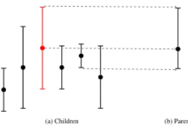
The confidence intervals in the tree represent the statistically plausible values in each node, hence the representative child can be interpreted as an “optimistic move” in a MAX node and a “pessimistic move” in a MIN node (assuming we play against the best possible adversary). This is reminiscent of the behavior of the UCT algorithm [17]. The construction of the confidence intervals and associated representative children are illustrated in Figure1.

(a) Children (b) Parent

Figure 1: Construction of confidence interval and representative child (in red) for a MAX node.

Input: a BAI algorithm Initialization: t= 0.

while not BAIStop({s ∈ C(s0)}) do Rt₊₁= BAIStep ({s ∈ C(s0)})

Sample the representative leaf Lt+1= ℓRt+1(t) Update the information about the arms. t= t + 1. end

Output: BAIReco({s ∈ C(s0)})

Figure 2: The BAI-MCTS architecture

2.2

The BAI-MCTS architecture

In this section we present the generic BAI-MCTS algorithm, whose sampling rule combines two ingredients: a best arm identification step which selects an action at the root, followed by a confidence based exploration step, that goes down the tree starting from this depth-one node in order to select the representative leaf for evaluation.

The structure of a BAI-MCTS algorithm is presented in Figure2. The algorithm depends on a Best Arm Identification (BAI) algorithm, and uses the three components of this algorithm:

• the sampling rule BAIStep(S) selects an arm in the set S

• the stopping rule BAIStop(S) returns True if the algorithm decides to stop • the recommendation rule BAIReco(S) selects an arm as a candidate for the best arm

In BAI-MCTS, the arms are the depth-one nodes, hence the information needed by the BAI algorithm to make a decision (e.g. BAIStep for choosing an arm, or BAIStop for stopping) is information about depth-one nodes, that has to be updated at the end of each round (last line in the while loop). Different BAI algorithms may require different information, and we now present two instances that rely on confidence intervals (and empirical estimates) for the value of the depth-one nodes.

2.3

UGapE-MCTS and LUCB-MCTS

Several Best Arm Identification algorithms may be used within BAI-MCTS, and we now present two variants, that are respectively based on the UGapE [8] and the LUCB [13] algorithms. These two algorithms are very similar in that they exploit confidence intervals and use the same stopping rule, however the LUCB algorithm additionally uses the empirical means of the arms, which within BAI-MCTS requires defining an estimate ˆVs(t) of the value of the depth-one nodes.

The generic structure of the two algorithms is similar. At round t+ 1 two promising depth-one nodes are computed, that we denote by b_tand c_t. Among these two candidates, the node whose confidence interval is the largest (that is, the most uncertain node) is selected:

Rt₊₁= argmax i∈{bt,ct}

[Ui(t) − Li(t)].

Then, following the BAI-MCTS architecture, the representative leaf of Rt+1(computed by going down the tree) is sampled: Lt+1= ℓRt+1(t). The algorithm stops whenever the confidence intervals of the two promising arms overlap by less than ǫ:

τ= inf {t ∈ N ∶ Uct(t) − Lb_t(t) < ǫ}, and it recommends ˆsτ= bτ.

In both algorithms that we detail below b_t represents a guess for the best depth-one node, while c_t is an “optimistic” challenger, that has the maximal possible value among the other depth-one nodes. Both nodes need to

UGapE-MCTS. In UGapE-MCTS, introducing for each depth-one node the index Bs(t) = max

s′_∈C(s0)/{s}Us

′(t) − Ls(t),

the promising depth-one nodes are defined as b_t= argmin

a∈C(s0)

Ba(t) and ct= argmax b∈C(s0)/{bt}

Ub(t).

LUCB-MCTS. In LUCB-MCTS, the promising depth-one nodes are defined as b_t= argmax a∈C(s0) ˆ Va(t) and ct= argmax b∈C(s0)/{bt} Ub(t),

where ˆVs(t) = ˆµℓs(t)(t) is the empirical mean of the reprentative leaf of node s. Note that several alternative definitions of ˆVs(t) may be proposed (such as the middle of the confidence interval Is(t), or maxa∈C(s)Vaˆ (t)), but our choice is crucial for the analysis of LUCB-MCTS, given in AppendixC.

3

Analysis of UGapE-MCTS

In this section we first prove that UGapE-MCTS and LUCB-MCTS are both (ǫ, δ)-correct. Then we give in Theorem 3a high-probability upper bound on the number of samples used by UGapE-MCTS. A similar upper bound is obtained for LUCB-MCTS in Theorem9, stated in AppendixC.

3.1

Choosing the Confidence Intervals

From now on, we assume that the confidence intervals on the leaves are of the form

Lℓ(t) = ˆµℓ(t) − ¿ Á Á Àβ(Nℓ(t),δ) 2Nℓ(t) and Uℓ(t) = ˆµℓ(t) + ¿ Á Á Àβ(Nℓ(t),δ) 2Nℓ(t) . (1)

β(s,δ) is some exploration function, that can be tuned to have a δ-PAC algorithm, as expressed in the following lemma, whose proof can be found in AppendixB.2

Lemma 2. Ifδ≤ max(0.1∣L∣,1), for the choice

β(s,δ) = ln(∣L∣/δ) + 3 ln ln(∣L∣/δ) + (3/2)ln(lns + 1) (2) both UGapE-MCTS and LUCB-MCTS satisfy P(V (s∗) − V (ˆsτ) ≤ ǫ) ≥ 1 − δ.

An interesting practical feature of these confidence intervals is that they only depend on the local number of draws Nℓ(t), whereas most of the BAI algorithms use exploration functions that depend on the number of rounds t. Hence the only confidence intervals that need to be updated at round t are those of the ancestors of the selected leaf, which can be done recursively.

Moreover, β(s,δ) scales with ln(ln(s)), and not ln(s), leveraging some tools recently introduced to obtain tighter confidence intervals [12,15]. The union bound overL (that may be an artifact of our current analysis) however makes the exploration function of Lemma2still a bit over-conservative and in practice, we recommend the use of β(s,δ) = ln (ln(es)/δ).

Finally, similar correctness results (with slightly larger exploration functions) may be obtained for confidence intervals based on the Kullback-Leibler divergence (see [5]), which are known to lead to better performance in standard best arm identification problems [16] and also depth-two tree search problems [10]. However, the sample complexity analysis is much more intricate, hence we stick to the above Hoeffding-based confidence intervals for the next section.

3.2

Complexity term and sample complexity guarantees

We first introduce some notation. Recall that s∗is the optimal action at the root, identified with the depth-one node satisfying V(s∗) = V (s0), and define the second-best depth-one node as s∗2= argmaxs∈C(s0)/{s∗}Vs. RecallP(s) denotes the parent of a node s different from the root. Introducing furthermore the set Anc(s) of all the ancestors of a node s, we define the complexity term by

H_ǫ∗(µ) ∶= ∑ ℓ∈L 1 ∆2 ℓ∨ ∆ 2 ∗∨ ǫ2 , where ∆∗ ∶= V (s ∗_{) − V (s}∗ 2) ∆ℓ ∶= maxs∈Anc(ℓ)/{s0}∣Vs− V (P(s))∣ (3) The intuition behind these squared terms in the denominator is the following. We will sample a leaf ℓ until we either prune it (by determining that it or one of its ancestors is a bad move), prune everyone else (this happens for leaves below the optimal arm) or reach the required precision ǫ.

Theorem 3. Letδ≤ min(1,0.1∣L∣). UGapE-MCTS using the exploration function (2) is such that, with probability larger than 1− δ, (V (s∗) − V (ˆsτ) < ǫ) and, letting ∆ℓ,ǫ= ∆ℓ∨ ∆∗∨ ǫ,

τ ≤ 8H_ǫ∗(µ)ln ∣L∣ δ + ∑_ℓ 16 ∆2_ℓ,ǫ ln ln 1 ∆2_ℓ,ǫ + 8H∗ ǫ(µ)[3 ln ln ∣L∣ δ + 2 lnln (8e ln ∣L∣δ + 24e lnln ∣L∣δ )] + 1.

Remark 4. If β(Na(t),δ) is changed to β(t,δ), one can still prove (ǫ,δ) correctness and furthermore upper bound the expectation of τ . However the algorithm becomes less efficient to implement, since after each leaf observation, ALL the confidence intervals have to be updated. In practice, this change lowers the probability of error but does not effect significantly the number of play-outs used.

3.3

Comparison with previous work

To the best of our knowledge1, the FindTopWinner algorithm [22] is the only algorithm from the literature de-signed to solve the best action identification problem in any-depth trees. The number of play-outs of this algorithm is upper bounded with high probability by

∑ ℓ∶∆ℓ>2ǫ( 32 ∆2 ℓ ln16∣L∣ ∆ℓδ + 1) + ∑_{ℓ∶∆ℓ≤2ǫ}( 8 ǫ2ln 8∣L∣ ǫδ + 1)

One can first note the improvement in the constant in front of the leading term in ln(1/δ), as well as the presence of the ln ln(1/∆ℓ,ǫ2) second order term, that is unavoidable in a regime in which the gaps are small [12]. The most interesting improvement is in the control of the number of draws of 2ǫ-optimal leaves (such that ∆ℓ ≤ 2ǫ). In UGapE-MCTS, the number of draws of such leaves is at most of order(ǫ ∨ ∆2∗)−1ln(1/δ), which may be significantly smaller than ǫ−1ln(1/δ) if there is a gap in the best and second best value. Moreover, unlike FindTopWinner and M-LUCB [10] in the depth two case, UGapE-MCTS can also be used when ǫ = 0, with provable guarantees.

Regarding the algorithms themselves, one can note that M-LUCB, an extension of LUCB suited for depth-two tree, does not belong to the class of BAI-MCTS algorithms. Indeed, it has a “reversed” structure, first computing the representative leaf for each depth-one node:∀s ∈ C(s0),Rs,t= ℓs(t) and then performing a BAI step over the representative leaves: ˜Lt₊₁= BAIStep(Rs,t, s∈ C(s0)). This alternative architecture can also be generalized to deeper trees, and was found to have empirical performance similar to BAI-MCTS. M-LUCB, which will be used as a benchmark in Section4, also distinguish itself from LUCB-MCTS by the fact that it uses an exploration rate

1_{In a recent paper, [11] independently proposed the LUCBMinMax algorithm, that differs from UGapE-MCTS and LUCB-MCTS only by}

the way the best guess btis picked. The analysis is very similar to ours, but features some refined complexity measure, in which∆ℓ(that is

the maximal distance between consecutive ancestors of the leaf, see (3)) is replaced by the maximal distance between any ancestors of that leaf.

that depends on the global time β(t,δ) and that btis the empirical maximin arm (which can be different from the arm maximizing ˆVs). This alternative choice is not yet supported by theoretical guarantees in deeper trees.

Finally, the exploration step of BAI-MCTS algorithm bears some similarity with the UCT algorithm [17], as it goes down the tree choosing alternatively the move that yields the highest UCB or the lowest LCB. However, the behavior of BAI-MCTS is very different at the root, where the first move is selected using a BAI algorithm. Another key difference is that BAI-MCTS relies on exact confidence intervals: each interval Is(t) is shown to contain with high probability the corresponding value Vs, whereas UCT uses more heuristic confidence intervals, based on the number of visits of the parent node, and aggregating all the samples from descendant nodes. Using UCT in our setting is not obvious as it would require to define a suitable stopping rule, hence we don’t include a comparison with this algorithm in Section4. A hybrid comparison between UCT and FindTopWinner is proposed in [22], providing UCT with the random number of samples used by the the fixed-confidence algorithm. It is shown that FindTopWinner has the advantage for hard trees that require many samples. Our experiments show that our algorithms in turn always dominate FindTopWinner.

3.4

Proof of Theorem

3

.

Letting Et = ⋂ℓ∈L(µℓ∈ Iℓ(t)) and E = ⋂t∈NEt, we upper bound τ assuming the eventE holds, using the following key result, which is proved in AppendixD.

Lemma 5. Lett∈ N. Et∩ (τ > t) ∩ (Lt+1= ℓ) ⇒ Nℓ(t) ≤ 8_∆β(Nℓ(t),δ)2 ℓ∨∆

2 ∗∨ǫ2.

An intuition behind this result is the following. First, using that the selected leaf ℓ is a representative leaf, it can be seen that the confidence intervals from sD= ℓ to s0are nested (Lemma11). Hence ifEtholds, V(sk) ∈ Iℓ(t) for all k = 1,... ,D, which permits to lower bound the width of this interval (and thus upper bound Nℓ(t)) as a function of the V(sk) (Lemma12). Then Lemma13exploits the mechanism of UGapE to further relate this width to ∆∗and ǫ.

Another useful tool is the following lemma, that will allow to leverage the particular form of the exploration function β to obtain an explicit upper bound on Nℓ(τ).

Lemma 6. Letβ(s) = C +3₂ln(1 + ln(s)) and define S = sup{s ≥ 1 ∶ aβ(s) ≥ s}. Then S≤ aC + 2a ln(1 + ln(aC)).

This result is a consequence of Theorem16stated in AppendixF, that uses the fact that for C ≥ −ln(0.1) and a≥ 8, it holds that

3 2

C(1 + ln(aC))

C(1 + ln(aC)) −3₂ ≤ 1.7995564 ≤ 2.

On the eventE, letting τℓbe the last instant before τ at which the leaf ℓ has been played before stopping, one has Nℓ(τ − 1) = Nℓ(τℓ) that satisfies by Lemma5

Nℓ(τℓ) ≤ 8β(Nℓ(τℓ),δ) ∆2 ℓ∨ ∆ 2 ∗∨ ǫ2 .

Applying Lemma6with a= aℓ= ∆2 8 ℓ∨∆ 2 ∗∨ǫ2 and C = ln ∣L∣ δ + 3 ln ln ∣L∣ δ leads to Nℓ(τ − 1) ≤ aℓ(C + 2 ln(1 + ln(aℓC))).

Letting ∆ℓ,ǫ= ∆ℓ∨ ∆∗∨ ǫ and summing over arms, we find τ = 1 + ∑ ℓ Nℓ(τ − 1) ≤ 1 + ∑ ℓ 8 ∆2_ℓ,ǫ ⎛ ⎜ ⎝ln ∣L∣ δ + 3 lnln ∣L∣δ + 2 ln ln ⎛ ⎜ ⎝8e ln∣L∣_δ + 3 lnln∣L∣_δ ∆2_ℓ,ǫ ⎞ ⎟ ⎠ ⎞ ⎟ ⎠ = 1 + ∑ ℓ 8 ∆2_ℓ,ǫ ⎛ ⎜ ⎝ln ∣L∣ δ + 2 lnln 1 ∆2_ℓ,ǫ ⎞ ⎟ ⎠+ 8H ∗ ǫ(µ)[3 ln ln ∣L∣ δ + 2 lnln (8e ln ∣L∣δ + 24e lnln ∣L∣δ )] . To conclude the proof, we remark that from the proof of Lemma2(see AppendixB.2) it follows that onE, V(s∗) − V (ˆsτ) < ǫ and that E holds with probability larger than 1 − δ.

4

Experimental Validation

In this section we evaluate the performance of our algorithms in three experiments. We evaluate on the depth-two benchmark tree from [10], a new depth-three tree and the random tree ensemble from [22]. We compare to the FindTopWinner algorithm from [22] in all experiments, and in the depth-two experiment we include the M-LUCB algorithm from [10]. Its relation to BAI-MCTS is discussed in Section3.3. For our BAI-MCTS algorithms and for M-LUCB we use the exploration rate β(s,δ) = ln∣L∣_δ + ln(ln(s) + 1) (a stylized version of Lemma2that works well in practice), and we use the KL refinement of the confidence intervals (1). To replicate the experiment from [22], we supply all algorithms with δ = 0.1 and ǫ = 0.01. For comparing with [10] we run all algorithms with ǫ= 0 and δ = 0.1∣L∣ (undoing the conservative union bound over leaves. This excessive choice, which might even exceed one, does not cause a problem, as the algorithms depend on_∣L∣δ = 0.1). In none of our experiments the observed error rate exceeds 0.1.

Figure3 shows the benchmark tree from [10, Section 5] and the performance of four algorithms on it. We see that the special-purpose depth-two M-LUCB performs best, very closely followed by both our new arbitrary-depth LUCB-MCTS and UGapE-MCTS methods. All three use significantly fewer samples than FindTopWinner. Figure4(displayed in AppendixAfor the sake of readability) shows a full 3-way tree of depth 3 with leafs drawn uniformly from[0,1]. Again our algorithms outperform the previous state of the art by an order of magnitude. Finally, we replicate the experiment from [22, Section 4]. To make the comparison as fair as possible, we use the proven exploration rate from (2). On 10K full 10-ary trees of depth 3 with Bernoulli leaf parameters drawn uniformly at random from[0,1] the average numbers of samples are: LUCB-MCTS 141811, UGapE-MCTS 142953 and FindTopWinner 2254560. To closely follow the original experiment, we do apply the union bound over leaves to all algorithms, which are run with ǫ = 0.01 and δ = 0.1. We did not observe any error from any algorithm (even though we allow 10%). Our BAI-MCTS algorithms deliver an impressive 15-fold reduction in samples.

5

Lower bounds and discussion

Given a treeT , a MCTS model is parameterized by the leaf values, µ ∶= (µℓ)ℓ∈L, which determine the best root action: s∗ = s∗(µ). For µ ∈ [0,1]∣L∣, We define Alt(µ) = {λ ∈ [0,1]∣L∣ ∶ s∗(λ) ≠ s∗(µ)}. Using the same technique as [9] for the classic best arm identification problem, one can establish the following (non explicit) lower bound. The proof is given in AppendixE.

Theorem 7. Assumeǫ= 0. Any δ-correct algorithm satisfies

E_µ[τ] ≥ T∗(µ)d(δ,1 − δ), where T∗(µ)−1∶= sup

w∈Σ∣L∣λ_∈Alt(µ)inf _ℓ∈L∑wℓd(µℓ, λℓ) (4) with Σk = {w ∈ [0,1]i ∶ ∑ki=1wi = 1} and d(x,y) = xln(x/y) + (1 − x)ln((1 − x)/(1 − y)) is the binary Kullback-Leibler divergence.

0.45 0.45 0.35 0.30 0.45 0.50 0.55 905 875 2941 798 199 200 2931 212 81 82 2498 92 0.35 0.40 0.60 629 630 2932 752 287 279 2930 248 17 17 418 22 0.30 0.47 0.52 197 193 1140 210 123 123 739 4 4 20 20 566 21

Figure 3: The 3× 3 tree of depth 2 that is the benchmark in [10]. Shown below the leaves are the average numbers of pulls for 4 algorithms: LUCB-MCTS (0.89% errors, 2460 samples), UGapE-MCTS (0.94%, 2419), FindTopWinner (0%, 17097) and M-LUCB (0.14%, 2399). All counts are averages over 10K repetitions with ǫ= 0 and δ = 0.1 ⋅ 9.

This result is however not directly amenable for comparison with our upper bounds, as the optimization prob-lem defined in Lemma7is not easy to solve. Note that d(δ,1−δ) ≥ ln(1/(2.4δ)) [15], thus our upper bounds have the right dependency in δ. For depth-two trees with K (resp. M ) actions for player A (resp. B), we can moreover prove the following result, that suggests an intriguing behavior.

Lemma 8. Assumeǫ= 0 and consider a tree of depth two with µ = (µi,j)1_{≤i≤K,1≤j≤M} such that ∀(i,j),µ1,1> µi,1, µi,1< µi,j. The supremum in the definition ofT∗(µ)−1can be restricted to

˜ ΣK,M∶= {w ∈ ΣK×M ∶ wi,j= 0 if i ≥ 2 and j ≥ 2} and T∗(µ)−1= max w∈˜Σ_K,M min i=2,...,K a=1,...,M [w1,ad(µ1,a, w1,aµ1,a+ wi,1µi,1 w1,a+ wi,1 )+wi,1

d(µi,1,w1,aµ1,a+ wi,1µi,1 w1,a+ wi,1 )] . It can be extracted from the proof of Theorem7 (see AppendixE) that the vector w∗(µ) that attains the supremum in (4) represents the average proportions of selections of leaves by any algorithm matching the lower bound. Hence, the sparsity pattern of Lemma8suggests that matching algorithms should draw many of the leaves much less thanO(ln(1/δ)) times. This hints at the exciting prospect of optimal stochastic pruning, at least in the asymptotic regime δ→ 0.

As an example, we numerically solve the lower bound optimization problem (which is a concave maximization problem) for µ corresponding to the benchmark tree displayed in Figure3to obtain

T∗(µ) = 259.9 and w∗ = (0.3633,0.1057,0.0532),(0.3738,0,0),(0.1040,0,0).

With δ = 0.1 we find kl(δ,1 − δ) = 1.76 and the lower bound is Eµ[τ] ≥ 456.9. We see that there is a potential improvement of at least a factor 4.

Future directions An (asymptotically) optimal algorithm for BAI called Track-and-Stop was developed by [9]. It maintains the empirical proportions of draws close to w∗(ˆµ), adding forced exploration to ensure ˆµ → µ. We

believe that developing this line of ideas for MCTS would result in a major advance in the quality of tree search algorithms. The main challenge is developing efficient solvers for the general optimization problem (4). For now, even the sparsity pattern revealed by Lemma8for depth two does not give rise to efficient solvers. We also do not know how this sparsity pattern evolves for deeper trees, let alone how to compute w∗(µ).

Acknowledgments. Emilie Kaufmann acknowledges the support of the French Agence Nationale de la Recherche (ANR), under grants ANR-16-CE40-0002 (project BADASS) and ANR-13-BS01-0005 (project SPADRO). Wouter Koolen acknowledges support from the Netherlands Organization for Scientific Research (NWO) under Veni grant 639.021.439.

References

[1] J-Y. Audibert, S. Bubeck, and R. Munos. Best Arm Identification in Multi-armed Bandits. In Proceedings of the 23rd Conference on Learning Theory, 2010.

[2] P. Auer, N. Cesa-Bianchi, and P. Fischer. Finite-time analysis of the multiarmed bandit problem. Machine Learning, 47(2):235–256, 2002.

[3] L. Borsoniu, R. Munos, and E. Páll. An analysis of optimistic, best-first search for minimax sequential decision making. In ADPRL14, 2014.

[4] C. Browne, E. Powley, D. Whitehouse, S. Lucas, P. Cowling, P. Rohlfshagen, S. Tavener, D. Perez, S. Samoth-rakis, and S. Colton. A survey of monte carlo tree search methods. IEEE Transactions on Computational Intelligence and AI in games,, 4(1):1–49, 2012.

[5] O. Cappé, A. Garivier, O-A. Maillard, R. Munos, and G. Stoltz. Kullback-Leibler upper confidence bounds for optimal sequential allocation. Annals of Statistics, 41(3):1516–1541, 2013.

[6] T. Cazenave. Sequential halving applied to trees. IEEE Transactions on Computational Intelligence and AI in Games, 7(1):102–105, 2015.

[7] E. Even-Dar, S. Mannor, and Y. Mansour. Action Elimination and Stopping Conditions for the Multi-Armed Bandit and Reinforcement Learning Problems. Journal of Machine Learning Research, 7:1079–1105, 2006. [8] V. Gabillon, M. Ghavamzadeh, and A. Lazaric. Best Arm Identification: A Unified Approach to Fixed Budget

and Fixed Confidence. In Advances in Neural Information Processing Systems, 2012.

[9] A. Garivier and E. Kaufmann. Optimal best arm identification with fixed confidence. In Proceedings of the 29th Conference On Learning Theory (COLT), 2016.

[10] A. Garivier, E. Kaufmann, and W.M. Koolen. Maximin action identification: A new bandit framework for games. In Proceedings of the 29th Conference On Learning Theory, 2016.

[11] Ruitong Huang, Mohammad M. Ajallooeian, Csaba Szepesvári, and Martin Müller. Structured best arm identification with fixed confidence. In 28th International Conference on Algorithmic Learning Theory (ALT), 2017.

[12] K. Jamieson, M. Malloy, R. Nowak, and S. Bubeck. lil’UCB: an Optimal Exploration Algorithm for Multi-Armed Bandits. In Proceedings of the 27th Conference on Learning Theory, 2014.

[13] S. Kalyanakrishnan, A. Tewari, P. Auer, and P. Stone. PAC subset selection in stochastic multi-armed bandits. In International Conference on Machine Learning (ICML), 2012.

[14] Z. Karnin, T. Koren, and O. Somekh. Almost optimal Exploration in multi-armed bandits. In International Conference on Machine Learning (ICML), 2013.

[15] E. Kaufmann, O. Cappé, and A. Garivier. On the Complexity of Best Arm Identification in Multi-Armed Bandit Models. Journal of Machine Learning Research, 17(1):1–42, 2016.

[16] E. Kaufmann and S. Kalyanakrishnan. Information complexity in bandit subset selection. In Proceeding of the 26th Conference On Learning Theory., 2013.

[17] L. Kocsis and C. Szepesvári. Bandit based monte-carlo planning. In Proceedings of the 17th European Conference on Machine Learning, ECML’06, pages 282–293, Berlin, Heidelberg, 2006. Springer-Verlag. [18] T.L. Lai and H. Robbins. Asymptotically efficient adaptive allocation rules. Advances in Applied

Mathemat-ics, 6(1):4–22, 1985.

[19] T. Pepels, T. Cazenave, M. Winands, and M. Lanctot. Minimizing simple and cumulative regret in monte-carlo tree search. In Computer Games Workshop, ECAI, 2014.

[20] Aske Plaat, Jonathan Schaeffer, Wim Pijls, and Arie de Bruin. Best-first fixed-depth minimax algorithms. Artificial Intelligence, 87(1):255 – 293, 1996.

[21] David Silver, Aja Huang, Chris J. Maddison, Arthur Guez, Laurent Sifre, George van den Driessche, Julian Schrittwieser, Ioannis Antonoglou, Veda Panneershelvam, Marc Lanctot, Sander Dieleman, Dominik Grewe, John Nham, Nal Kalchbrenner, Ilya Sutskever, Timothy Lillicrap, Madeleine Leach, Koray Kavukcuoglu, Thore Graepel, and Demis Hassabis. Mastering the game of go with deep neural networks and tree search. Nature, 529:484–489, 2016.

[22] K. Teraoka, K. Hatano, and E. Takimoto. Efficient sampling method for monte carlo tree search problem. IEICE Transactions on Infomation and Systems, pages 392–398, 2014.

[23] W.R. Thompson. On the likelihood that one unknown probability exceeds another in view of the evidence of two samples. Biometrika, 25:285–294, 1933.

A

Numerical Results for a Depth Three Tree

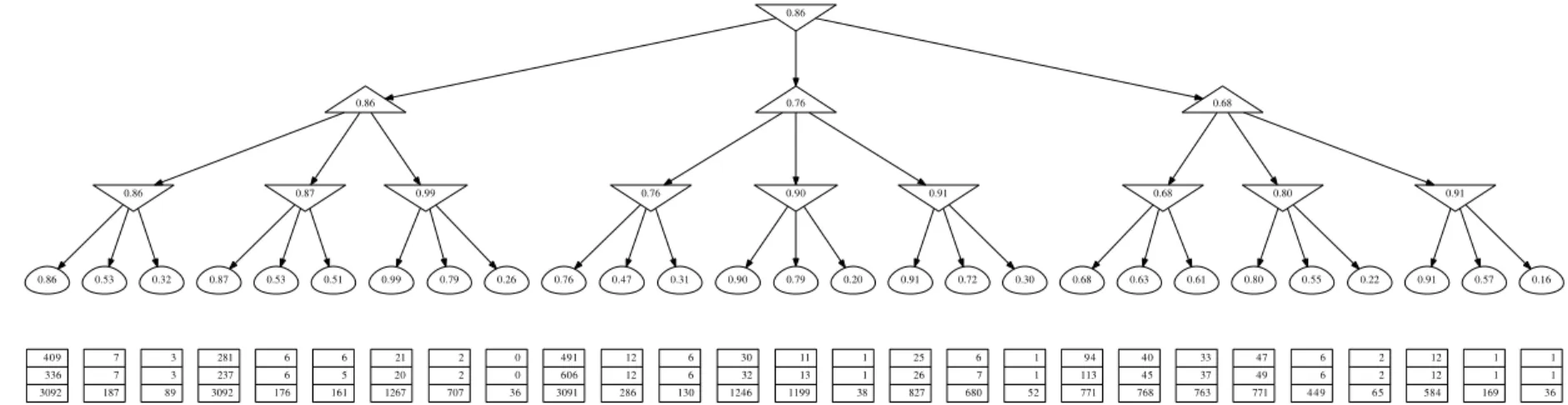
The results for our experiments on a depth-three tree are displayed in Figure4.

B

Confidence Intervals

B.1

Proof of Proposition

1

The proof proceeds by induction. Let the inductive hypothesis beHd=“for all the nodes s at (graph) distance d from a leaf, Vs∈ Is(t)”.

H0clearly holds by definition ofEt. Now let d such thatHdholds and let s be at distance d + 1 of a leaf. Then all s′∈ C(s) are at distance at most d from a leaf and using the inductive hypothesis,

∀c∈ C(s), Lc(t) ≤ Vc≤ Uc(t).

Assume that s is a MAX node. Using that Us(t) = maxc∈C(s)Uc(t), one has c ∈ C(s), Vc ≤ Uc(t) ≤ Us(t). By definition, Vs = maxc∈C(s)Vc, thus it follows that Vs ≤ Us(t). Still by definition of Vs, it holds that ∀c ∈ C(s),Lc(t) ≤ Vc≤ Vsand finally, as Ls(t) = maxc∈C(s)Lc(t), Ls(t) ≤ Vs≤ Us(t). A similar reasoning yields the same conclusion if s is a MIN node, thusHd+1holds.

0.86 0.86 0.76 0.68 0.86 0.87 0.99 0.86 0.53 0.32 4 0 9 336 3092 7 7 187 3 3 89 0.87 0.53 0.51 281 237 3092 6 6 176 6 5 161 0.99 0.79 0.26 21 20 1267 2 2 707 0 0 36 0.76 0.90 0.91 0.76 0.47 0.31 491 606 3091 12 12 286 6 6 130 0.90 0.79 0.20 30 32 1246 11 13 1199 1 1 38 0.91 0.72 0.30 25 26 827 6 7 680 1 1 52 0.68 0.80 0.91 0.68 0.63 0.61 9 4 113 771 4 0 4 5 768 33 37 763 0.80 0.55 0.22 4 7 4 9 771 6 6 4 4 9 2 2 6 5 0.91 0.57 0.16 12 12 584 1 1 169 1 1 36

Figure 4: Our benchmark 3-way tree of depth 3. Shown below the leaves are the numbers of pulls of 3 algorithms: LUCB-MCTS (0.72% errors, 1551 samples), UGapE-MCTS (0.75%, 1584), and FindTopWinner (0%, 20730). Numbers are averages over 10K repetitions with ǫ= 0 and δ = 0.1 ⋅ 27.

1

B.2

Proof of Lemma

2

Let

Et= ⋂

ℓ∈L(µℓ∈ Iℓ(t)) and E = ⋂t∈NEt.

Using Proposition1, onEt, for all s∈ T , Vs∈ Is(t). If the algorithm stops at some time t, as Lb_t(t) > Uc_t(t) − ǫ, the outputted action, ˆsτ= bt, satisfies Lˆsτ(t) > Us′(t) − ǫ, for all s′≠ ˆs_τ. AsE holds, one obtains

V(ˆsτ) ≥ max s′_≠ˆsτV(s

′_{) − ǫ,}

and ˆsτis an ǫ-maximin action. Hence, the algorithm is correct onE. The error probability is thus upper bounded by P(Ec) ≤ P (∃ℓ ∈ L,∃t ∈ N ∶ ∣ˆµ_ℓ(t) − µ_ℓ∣ >√_β(N_ℓ(t),δ)/(2N_ℓ(t))) ≤ ∑ ℓ∈L P(∃s ∈ N ∶ 2s(ˆµ_{ℓ,s− µℓ})2> β(s,δ)) ≤ 2∣L∣P (∃s ∈ N ∶ Ss> √ 2σ2_sβ(s,δ)),

where Ss= X1+ ⋅ ⋅ ⋅ + Xsis a martingale with σ2-subgaussian increments, with σ2= 1/4. It was shown in [15] that for δ≤ 0.1, if β(t,δ) = ln(1 δ) + 3 lnln( 1 δ) + (3/2)ln(ln(s) + 1), one has P(∃s ∈ N ∶ Ss> √

2σ2_sβ(s,δ)) ≤ δ, which concludes the proof.

C

Sample complexity analysis of LUCB-MCTS

We provide an analysis of a slight variant of LUCB-MCTS that may stop at even rounds only and for t∈ 2N draws the representative leaf of the two promising depth-one nodes:

Lt₊₁= ℓb_t(t) and Lt+2= ℓc_t(t). (5) The stopping rule is then τ = inf {t ∈ 2N∗∶ Uc_t(t) − Lb_t(t) < ǫ}.

For this algorithm, our sample complexity guarantee features a slightly different complexity term. For a leaf ℓ= s0s1. . . sD, we first introduce

˜

∆ℓ= max

s∈Anc(ℓ)/{s0,s1}∣V (s) − V (P(s))∣,

a quantity that differs from ∆ℓonly by the fact that the maximum doesn’t take into account the gap between the root and the depth-one ancestor of ℓ. Then ˜H_ǫ∗(µ) is defined similarly as H_ǫ∗(µ) by

˜ H_ǫ∗(µ) = ∑ ℓ∈L 1 ˜ ∆2 ℓ∨ ∆ 2 ∗∨ ǫ2 .

Theorem 9. Letδ≤ min(1,0.1∣L∣). LUCB-MCTS using the exploration function (2) and selecting the two promis-ing leaves at each round is such that, with probability larger than 1 − δ,(V (s∗) − V (ˆsτ) < ǫ) and

τ≤ 16 ˜H_ǫ∗(µ)[ln ∣L∣ δ + 3 ln ln ∣L∣ δ + 2 ln ln(16e ˜H ∗ ǫ(µ)(ln ∣L∣_δ + 3 ln ln∣L∣_δ ))] .

Proof. The analysis follows the same lines as that of UGapE-MCTS, yet it relies on a slightly different key result, proved in the next section. LettingEt= ∩ℓ∈L(µℓ∈ Iℓ(t)) as in the proof of Theorem3and definingE = ∩t∈2N∗Et, one can state the following.

Lemma 10. Lett∈ 2N. Et∩(τ > t) ⇒ ∃ℓ ∈ {Lt+1, Lt+2} ∶ Nℓ(t) ≤ 8β(t,δ) ˜ ∆2 ℓ∨ ∆ 2 ∗∨ ǫ2 .

Let T be a deterministic time. We upper bound τ assuming the eventE holds. Using Lemma10and the fact that for every even t,(τδ> t) = (τδ> t + 1) by definition of the algorithm, one has

min(τ,T ) = T ∑ t=01(τ >t)= 2 ∑t∈2N t≤T 1(τδ>t)= 2 ∑ t∈2N t≤T 1_{(∃ℓ∈{Lt+1,Lt+2}∶Nℓ(t)≤2β(t,δ)/( ˜}∆2 ℓ∨∆ 2 ∗ǫ2)) ≤ 2 ∑ t∈2N t≤T ∑ ℓ∈L1(Lt+1=ℓ)∪(Lt+2=ℓ)1(Nℓ(t)≤8β(T,δ)/( ˜∆ 2 ℓ∨∆ 2 ∗ǫ2₎₎ ≤ 16 ∑ ℓ∈L 1 ˜ ∆2 ℓ∨ ∆ 2 ∗∨ ǫ2 β(T,δ) = 16 ˜H_ǫ∗(µ)β(T,δ).

For any T such that 16 ˜Hǫ∗(µ)β(T,δ) < T , one has min(τ,T ) < T , which implies τ < T . Therefore τ≤ sup{t ∈ N ∶ 16 ˜H_ǫ∗(µ)β(t,δ) ≥ t}.

Just like in the analysis of UGapE-MCTS, the conclusion now follows from Lemma6, applied with a= 16 ˜H_ǫ∗(µ) and C= ln(∣L∣/δ) + 3 lnln(∣L∣/δ), which yields

τ≤ 16 ˜H_ǫ∗(µ)[ln ∣L∣ δ + 3 ln ln ∣L∣ δ + 2 ln ln(16e ˜H ∗ ǫ(µ)(ln ∣L∣ δ + 3 ln ln ∣L∣ δ ))] . Using thatP(E) ≥ 1 − δ and that the algorithm is correct on E yields the conclusion.

D

Proof of Lemma

5

and Lemma

10

We first state Lemma12, that holds for both UGapE and LUCB-MCTS and is a consequence of the definition of the exploration procedure. This result builds on the following lemma, that expresses the fact that along a path from the root to a representative leaf, the confidence intervals are nested.

Lemma 11. Lett∈ N and s0, s1, . . . , sDbe a path from the root down to a leafℓ= sD. (ℓs1(t) = sD) ⇒ (∀k = 2,... ,D, Isk−1(t) ⊆ Isk(t))

Lemma 12. Lett∈ N and s0, s1, . . . , sDbe a path from the root down to a leafℓ= sD. IfEtholds andℓ is selected at round_{t + 1 (UGapE) or if t is even and ℓ}∈ {L_t+1, Lt+2} (LUCB), then

¿ Á Á

À2β(Nℓ(t),δ)

Nℓ(t) ≥ maxk=2...D∣V (sk) − V (sk−1)∣.

UGapE-MCTS: proof of Lemma5. The following lemma is specific to UGapE-MCTS. We let s0, s1, . . . , sD be a path down to a leaf ℓ= sD.

Lemma 13. Lett∈ N. If Etholds and UGapE-MCTS has not stopped aftert observations, that is(τ > t), (Lt+1= ℓ) ⇒⎛⎜ ⎝ ¿ Á Á À8β(Nℓ(t),δ) Nℓ(t) ≥ max (∆∗, V(s0) − V (s1),ǫ) ⎞ ⎟ ⎠

Putting together Lemma12and Lemma13and using that ∆ℓ= max (V (s0) − V (s1), max k=2...D∣V (sk) − V (sk−1)∣) one obtains Et∩(τ > t) ∩ (Lt+1= ℓ) ⇒ ⎛ ⎜ ⎝ ¿ Á Á À8β(Nℓ(t),δ) Nℓ(t) ≥ max (∆ℓ, ∆∗, ǫ) ⎞ ⎟ ⎠, which yields the proof of Lemma5by inverting the bound.

LUCB-MCTS: proof of Lemma10. The following lemma is specific to the LUCB-MCTS algorithm. It can be viewed as a generalization of Lemma 2 in [13].

Lemma 14. Lett ∈ 2N and let γ ∈ [V (s∗2),V (s∗)]. If Et holds and LUCB-MCTS has not stopped after t observations, that is(τ > t), then

∃ℓ∈ {Lt+1, Lt+2} ∶ (γ ∈ Iℓ(t)) ∩ ⎛ ⎜ ⎝ ¿ Á Á À2β(t,δ) Nℓ(t) ≥ǫ ⎞ ⎟ ⎠. Choosing γ= V(s ∗_{)+V (s}∗₂₎

2 and letting sℓbe the depth-one ancestor of ℓ, onEtit holds that V(sℓ) ∈ Iℓ(t) (by Lemma11) and (γ ∈ Iℓ(t)) ⇒ ⎛⎜ ⎝ ¿ Á Á À2β(t,δ) Nℓ(t) ≥ ∣V(sℓ) − γ∣ ⎞ ⎟ ⎠ ⇒ ⎛⎜ ⎝ ¿ Á Á À2β(t,δ) Nℓ(t) ≥ V(s∗) − V (s∗2) 2 ⎞ ⎟ ⎠.

Recall ∆∗= V (s∗) − V (s∗2). By Lemma14, onEt∩(τ > t), there exists ℓ ∈ {Lt+1, Lt+2} such that ¿

Á Á À8β(t,δ)

Nℓ(t) ≥max(∆∗, ǫ). (6)

Moreover, noting that for a leaf ℓ= s0, s1, . . . , sD, ˜

∆ℓ= max

k=2,...,D∣V (sk) − V (sk−1)∣ a consequence of Lemma12is that for ℓ∈ {Lt+1, Lt+2},

¿ Á Á À2β(t,δ) Nℓ(t) ≥ ˜ ∆ℓ. (7)

Combining (6) and (7) yields

Et∩(τ > t) ⇒ ∃ℓ ∈ {Lt+1, Lt+2} ∶ ¿ Á Á À8β(t,δ) Nℓ(t) ≥max( ˜∆ℓ, ∆∗, ǫ) , which yields the proof of Lemma10by inverting the bound.

D.1

Proof of Lemma

11

.

The leaf ℓ is the representative of the depth 1 node s1, therefore the path s1, . . . , sDis such that csk−1(t) = sk for all k= 2,... ,D. Using the way the representative are build, we now show that

∀k∈ {2,... ,D}, Isk−1(t) ⊆ Isk(t).

If sk−1is a MAX node, Usk−1(t) = Usk(t) by definition and Lsk−1(t) = maxs_∈C(sk−1)Ls(t) ≥ Lsk(t). Similarly, if s_k−1is a MIN node, Lsk−1(t) = Lsk(t) by definition and Usk−1(t) = mins_∈C(sk−1)Us(t) ≤ Usk(t), so that in both casesIsk−1(t) ⊆ Isk(t).

D.2

Proof of Lemma

12

.

Let ℓ∈ L be a leaf that is sampled based on the information available at round t. In particular, as ℓ is a representative leaf of the depth 1 node s1, the path s1, . . . , sDis such that csk−1(t) = skfor all k= 2,... ,D. Let k = 2,... ,D. If sk−1∈ {2,...,D} is a MAX node, it holds by definition of the representative children that, for all s′∈ C(sk−1),

Usk(t) ≥ Us′(t).

Now, from Lemma11one has Uℓ(t) ≥ Usk(t) and from Proposition1asEtholds, one has

∀s∈ T , Vs∈ Is(t). (8)

Using these two ingredients yields

Uℓ(t) ≥ V (s′) Lℓ(t) + 2 ¿ Á Á Àβ(Nℓ(t),δ) 2Nℓ(t) ≥ V (s ′₎ Lsk(t) + 2 ¿ Á Á Àβ(Nℓ(t),δ) 2Nℓ(t) ≥ V (s ′₎ V(sk) + 2 ¿ Á Á Àβ(Nℓ(t),δ) 2Nℓ(t) ≥ V (s ′_). Thus ¿ Á Á À2β(Nℓ(t),δ) Nℓ(t) ≥ s′_∈C(sk−1)max V(s ′_{) − V (s} k) = V (sk−1) − V (sk) ≥ 0.

If sk−1is a MIN node, a similar reasoning show that ¿

Á Á

À2β(Nℓ(t),δ)

Nℓ(t) ≥ V (sk) − V (sk−1) ≥ 0. Putting everything together yields

¿ Á Á

À2β(Nℓ(t),δ)

D.3

Proof of Lemma

13

.

We first prove the following intermediate result, that generalizes Lemma 4 in [8]. Lemma 15. For allt∈ N∗, the following holds

ifRt+1= bt then Uc_t(t) ≤ Ub_t(t) ifR_t+1= ct then Lct(t) ≤ Lbt(t)

Proof. Assume c_tis selected (i.e. Rt₊₁= ct) and Lct(t) > Lb_t(t). As the confidence interval on V (ct) is larger than the confidence intervals on V(bt) (ctis selected), this also yields Uc_t(t) > Ub_t(t). Hence

Bb_t(t) = Uc_t(t) − Lb_t(t) > Ub_t(t) − Lc_t(t). Also, by definition of c_t, Uct(t) ≥ Ub(t). Hence

Bb_t(t) > max b≠ct

Ub(t) − Lc_t(t) = Bc_t(t),

which contradicts the definition of b_t. Thus, we proved by contradiction that Lct(t) ≥ Lb_t(t). A similar reasoning can be used to prove that Rt₊₁= bt ⇒ Uct(t) ≤ Ub_t(t).

A simple consequence of Lemma15is the fact that, onEt∩(τ > t), (Lt+1= ℓ) ⇒ ⎛ ⎜ ⎝ ¿ Á Á À2β(Nℓ(t),δ) Nℓ(t) > ǫ ⎞ ⎟ ⎠. (9)

Indeed, as the algorithm doesn’t stop after t rounds, it holds that Uc_t(t) − Lb_t(t) > ǫ. If ℓ is the arm selected at round t + 1, ℓ= ℓRt+1(t) and one can prove using Lemma15that URt+1(t) − LRt+1(t) > ǫ (by distinguishing two cases). Finally, asEtholds, by Lemma11,IRt+1(t) ⊆ Iℓ(t). Hence Uℓ(t) − Lℓ(t) > ǫ, and (9) follows using the particular form of the confidence intervals.

To complete the proof, we now show that (Lt+1= ℓ) ⇒ ⎛ ⎜ ⎝ ¿ Á Á À8β(Nℓ(t),δ) Nℓ(t) > max(∆∗, V(s0) − V (s1) ⎞ ⎟ ⎠. (10)

by distinguishing several cases.

Case 1:s∗∉ Anc(ℓ) and Rt+1= ct. Using that the algorithm doesn’t stop yields Lct(t) − Ub_t(t) + 2(Uc_t(t) − Lc_t(t)) > ǫ. AsEtholds, Lc_t(t) ≤ V (ct) = V (s1) and Ub

t(t) ≥ V (bt). Therefore, if b_t= s∗it holds that

2(Uct(t) − Lct(t)) > V (s∗) − V (s1) + ǫ. If b_t≠ s∗, by definition of c_tone has

Uct(t) ≥ Us∗(t) ≥ V (s∗), hence

Lct(t) + (Uc_t(t) − Lc_t(t)) ≥ V (s∗) V(s1) + (Uc_t(t) − Lc_t(t)) ≥ V (s∗).

Thus, recalling that V(s0) = V (s∗), whatever the value of bt, one obtains 2(Uct(t) − Lct(t)) ≥ V (s0) − V (s1). From Lemma11the width ofIc_t(t) is upper bounded by the width of Iℓ(t), hence

2(Uℓ(t) − Lℓ(t)) ≥ V (s0) − V (s1). (11) Case 2:s∗∉ Anc(ℓ) and Rt+1= bt. As s∗≠ bt, by definition of ctone has

Uct(t) ≥ Us∗(t) ≥ V (s∗). Hence, using Lemma15,

Ub_t(t) − Lb_t(t) ≥ Uct(t) − Lbt(t) ≥ V (s∗) − V (s1), asEtholds. Finally, by Lemma11,

Uℓ(t) − Lℓ(t) ≥ V (s0) − V (s1). (12) Case 3:s∗∈ Anc(ℓ) and Rt+1= bt. One has b_t= s∗. Using that the algorithm doesn’t stop yields

Lct(t) − Ubt(t) + 2(Ubt(t) − Lbt(t)) > ǫ.

AsEtholds, Ub_t(t) ≤ V (s∗) and Lc_t(t) ≤ V (ct) ≤ V (s∗2). Therefore, if bt= s∗it holds that 2(Ubt(t) − Lb_t(t)) > V (s∗) − V (s∗2) + ǫ.

and by Lemma11

2(Uℓ(t) − Lℓ(t)) ≥ V (s∗) − V (s∗2). (13) Case 4:s∗∈ Anc(ℓ) and Rt+1= ct. One has c_t= s∗. Using Lemma15yields

Uc_t(t) − Lc_t(t) ≥ Uc_t(t) − Lb_t(t) ≥ V (s∗) − V (s∗2), asEtholds and V(bt) ≤ V (s∗2). Finally, by Lemma11,

Uℓ(t) − Lℓ(t) ≥ V (s∗) − V (s∗2). (14) Combining (11)-(14), we see that in all four cases

2(Uℓ(t) − Lℓ(t)) ≥ max(V (s∗) − V (s∗2),V (s0) − V (s1)),

as for s∗∉ Anc(ℓ), V (s0) − V (s1) = V (s∗) − V (s1) ≥ V (s∗) − V (s∗2), and for s∗∈ Anc(ℓ), V (s0) − V (s1) = 0. Using the expression of the confidence intervals and recalling that ∆∗= V (s∗) − V (s∗2), one obtains

4 ¿ Á Á Àβ(Nℓ(t),δ) 2Nℓ(t) ≥max(∆∗, V(s0) − V (s1)) which proves (10).

D.4

Proof of Lemma

14

.

Fix γ ∈ [V (s∗2),V (s∗)] and assume Et∩(τ > t) holds. We assume (by contradiction) that γ doesn’t belong to ILt+1(t) nor to ILt+2(t). There are four possibilities:

• LLt+1(t) > γ and LLt+2(t) > γ. As Etholds and Lt+1and Lt+2are representative, it yields that there exists two nodes s∈ C(s0) such that Vs> γ, which contradicts the definition of γ.

• ULt+1(t) < γ and ULt+2(t) < γ. From the definition of ct+1, it yields that for all s∈ C(s0), Us(t) < γ and as Etholds one obtains Vs< γ for all s ∈ C(s0), which contradicts the definition of γ.

• LLt+1(t) > γ and γ > ULt+2(t). This implies that LLt+1(t) > ULt+2(t) and that Lbt(t) > Uct(t) (by Lemma11and the fact that Lt₊₁and Lt₊₂are representative leaves). This yields(τ ≤ t) and a contradiction. • ULt+1(t) < γ and γ < LLt+2(t). This implies in particular that ˆµLt+1(t) < ˆµLt+2(t). Thus ˆV (bt, t) < ˆV (ct, t),

which contradicts the definition of b_t.

Hence, we just proved by contradiction that there exists ℓ∈ {Lt+1, Lt+2} such that γ ∈ Iℓ(t). To prove Lemma14, it remains to establish the following three statements.

1. (γ ∈ ILt+1(t)) ∩ (γ ∈ ILt+2(t)) ⇒ (∃ℓ ∈ {Lt+1, Lt+2} ∶ √ 2_β(t,δ) Nℓ(t) > ǫ) 2. (γ ∈ ILt+1(t)) ∩ (γ ∉ ILt+2(t)) ⇒ ( √ 2_β(t,δ) N_Lt+1(t) > ǫ) 3. (γ ∉ ILt+1(t)) ∩ (γ ∈ ILt+2(t)) ⇒ ( √ 2_β(t,δ) N_Lt+2(t) > ǫ)

Statement 1. As the algorithm doesn’t stop, Uc_t(t) − Lb_t(t) > ǫ. Hence

ULt+2(t) − LLt+1(t) > ǫ ˆ µLt+2(t) + ¿ Á Á Àβ(NLt+2(t),δ) 2NLt+2(t) − ˆµLt+1(t) + ¿ Á Á Àβ(NLt+1(t),δ) 2NLt+1(t) > ǫ ¿ Á Á Àβ(NLt+2(t),δ) 2NLt+2(t) + ¿ Á Á Àβ(NLt+1(t),δ) 2NLt+1(t) > ǫ using that by definition of b_t, ˆµLt+2(t) < ˆµLt+1(t). Hence, there exists ℓ ∈ {Lt+1, Lt+2} such that

¿ Á Á Àβ(Nℓ(t),δ) 2Nℓ(t) > ǫ 2 ⇒ ¿ Á Á À2β(t,δ) Nℓ(t) >ǫ.

Statement 2. We consider two cases and first assume that γ ∈ ILt+1(t) and γ ≥ ULt+2(t). Using the fact that the algorithm doesn’t stop at round t, the following events hold

(ULt+2(t) − LLt+1(t) > ǫ) ∩ (ULt+1(t) > γ) ∩ (ULt+2(t) ≤ γ)

⇒ (ULt+2(t) − LLt+1(t) > ǫ) ∩ (ULt+1(t) > γ) ∩ (ULt+2(t) − LLt+1(t) + LLt+1(t) ≤ γ) ⇒ (ULt+1(t) > γ) ∩ (LLt+1(t) ≤ γ − ǫ) ⇒ (ULt+1(t) − LLt+1(t) > ǫ) ⇒ ⎛⎜ ⎝ ¿ Á Á À 2β(t,δ) NLt+1(t) >ǫ ⎞ ⎟ ⎠.

The second case is γ∈ ILt+1(t) and γ ≤ LLt+2(t). Then the following holds (ULt+2(t) − LLt+1(t) > ǫ) ∩ (LLt+1(t) ≤ γ) ∩ (LLt+2(t) ≥ γ) ⇒ (LLt+1(t) ≤ γ) ∩ (ULt+2(t) + LLt+2(t) − LLt+1(t) > γ + ǫ) ⇒ (LLt+1(t) ≤ γ) ∩⎛⎜ ⎝2ˆµLt+2(t) − ˆµLt+1(t) + ¿ Á Á À2β(NLt+1(t),δ) 2NLt+1(t) > γ + ǫ ⎞ ⎟ ⎠ ⇒ (LLt+1(t) ≤ γ) ∩⎛⎜ ⎝µLt+1(t) +ˆ ¿ Á Á À2β(NLt+1(t),δ) 2NLt+1(t) > γ + ǫ ⎞ ⎟ ⎠ ⇒ (ULt+1(t) − LLt+1(t) > ǫ),

where the third implication uses the fact that ˆµLt+2(t) ≤ ˆµLt+1(t).

Statement 3. We consider two cases and first assume that γ ∈ ILt+2(t) and γ ≤ LLt+1(t). Using the fact that the algorithm doesn’t stop at round t, the following events hold

(ULt+2(t) − LLt+1(t) > ǫ) ∩ (LLt+1(t) ≥ γ) ∩ (LLt+2(t) ≤ γ) ⇒ (ULt+2(t) > γ + ǫ) ∩ (LLt+2(t) ≤ γ) ⇒ (ULt+2(t) − LLt+2(t) > ǫ) ⇒ ⎛⎜ ⎝ ¿ Á Á À 2β(t,δ) NLt+2(t) >ǫ ⎞ ⎟ ⎠.

The second case is γ∈ ILt+2(t) and γ ≥ ULt+1(t). Then the following holds

(ULt+2(t) − LLt+1(t) > ǫ) ∩ (ULt+2(t) ≥ γ) ∩ (γ ≥ ULt+1(t)) ⇒ (ULt+2(t) − (LLt+1(t) + ULt+1(t)) > ǫ − γ) ∩ (ULt+2(t) ≥ γ) ⇒ ⎛⎜ ⎝µˆLt+2(t) + ¿ Á Á À2β(NLt+2(t),δ) 2NLt+2(t) − 2ˆµLt+1(t) > ǫ − γ ⎞ ⎟ ⎠∩(ULt+2(t) ≥ γ) ⇒ ⎛⎜ ⎝−ˆµLt+2(t) + ¿ Á Á À2β(NLt+2(t),δ) 2NLt+2(t) > ǫ − γ ⎞ ⎟ ⎠∩(ULt+2(t) ≥ γ) ⇒ (ULt+2(t) − LLt+2(t) > ǫ),

where the third implication uses the fact that ˆµLt+2(t) ≤ ˆµLt+1(t).

E

Proof of the lower bounds

E.1

Proof of Theorem

7

Theorem 7 follows from considering the best possible change of distribution λ ∈ Alt(µ). The expected log-likelihood ratio of the observations until τ under a model parameterized by µ and a model parameterized by λ is

E_µ[L_τ(µ,λ)] = ∑ ℓ∈L

E_µ[N_ℓ(τ)]d(µℓ, λℓ),

where Nℓ(t) is the number of draws of the leaf ℓ until round t. Using Lemma 1 of [15], for any eventE in the filtration generated by τ ,

As the strategy is δ-correct, lettingE = (ˆsτ = s∗(µ)) one has Pµ(E) ≥ 1 − δ and Pλ(E) ≤ δ (under this model, s∗(µ) is not the best action at the root under the model parameterized by λ). Using monotonicity properties of the Bernoulli KL-divergence, one obtains, for any λ∈ Alt(µ),

∑ ℓ∈L

E_µ[N_ℓ(τ)]d(µ_{ℓ, λℓ}) ≥ d(1 − δ,δ).

Then, one can write

inf λ∈Alt(µ)_ℓ∑_∈LEµ[Nℓ(τ)]d(µℓ, λℓ) ≥ d(1 − δ,δ) E_µ[τ] inf λ∈Alt(µ)_ℓ∈L∑ E_µ[N_ℓ(τ)] E_µ[τ] d(µℓ, λℓ) ≥ d(1 − δ,δ) E_µ[τ]⎛

⎝wsup∈Σ∣L∣λ_∈Alt(µ)inf _ℓ∈L∑

E_µ[Nℓ(τ)] E_µ[τ] d(µℓ, λℓ) ⎞ ⎠ ≥ d(1 − δ,δ), using that∑ℓ∈L Eµ[Nℓ(τ )]

Eµ[τ ] = 1. This concludes the proof.

One can also note that for an algorithm to match the lower bound, all the inequalities above should be equalities. In particular one would need w_ℓ∗(µ) ≃ Eµ[Nℓ(τ )]

E_{µ[τ ]} , where w∗ℓ(µ) is a maximizer in the definition of T∗(µ)−1in (4).

E.2

Proof of Lemma

8

In the particular case of a depth-two tree with K actions for player A and M actions for player B, T∗(µ)−1= sup w_∈ΣK×M inf λ∈Alt(µ) K ∑ k=1 K ∑ m=1 wk,md(µk,m, λk,m). From the particular structure of µ, the best action at the root is action i= 1. Hence

Alt(µ) = {λ ∶ ∃a ∈ {1,...,M},∃i ∈ {2,... ,K} ∶ ∀j ∈ {1,... ,M},λ1,a< λi,j}. It follows that T∗(µ)−1 = sup w∈ΣK×Ma∈{1,...,M}min i∈{2,...,K} inf λ∶∀j,λ1,a<λi,j K ∑ k=1 M ∑ m=1 wk,md(µk,m, λk,m) = sup w∈ΣK×Ma∈{1,...,M}min i∈{2,...,K} inf λ∶∀j,λ1,a<λi,j ⎡⎢ ⎢⎢ ⎣w1,ad(µ1,a, λ1,a) + M ∑ j=1

wi,jd(µi,j, λi,j)⎤⎥⎥⎥ ⎦ ´¹¹¹¹¹¹¹¹¹¹¹¹¹¹¹¹¹¹¹¹¹¹¹¹¹¹¹¹¹¹¹¹¹¹¹¹¹¹¹¹¹¹¹¹¹¹¹¹¹¹¹¹¹¹¹¹¹¹¹¹¹¹¹¹¹¹¹¹¹¹¹¹¹¹¹¹¹¹¹¹¹¹¹¹¹¹¹¹¹¹¹¹¹¹¹¹¹¹¹¹¹¹¹¹¹¹¹¹¹¹¹¹¹¹¹¹¹¹¹¹¹¹¹¹¹¹¹¹¹¹¹¹¹¹¹¹¹¹¹¹¹¹¹¹¹¹¹¹¹¹¹¹¹¹¹¹¹¹¹¹¹¹¹¹¹¹¹¹¹¹¹¹¹¹¹¹¹¹¹¹¹¸¹¹¹¹¹¹¹¹¹¹¹¹¹¹¹¹¹¹¹¹¹¹¹¹¹¹¹¹¹¹¹¹¹¹¹¹¹¹¹¹¹¹¹¹¹¹¹¹¹¹¹¹¹¹¹¹¹¹¹¹¹¹¹¹¹¹¹¹¹¹¹¹¹¹¹¹¹¹¹¹¹¹¹¹¹¹¹¹¹¹¹¹¹¹¹¹¹¹¹¹¹¹¹¹¹¹¹¹¹¹¹¹¹¹¹¹¹¹¹¹¹¹¹¹¹¹¹¹¹¹¹¹¹¹¹¹¹¹¹¹¹¹¹¹¹¹¹¹¹¹¹¹¹¹¹¹¹¹¹¹¹¹¹¹¹¹¹¹¹¹¹¹¹¹¹¹¹¹¹¹¹¶

∶=Fa,i(µ,w)

. (15)

Indeed, in the rightmost constrained minimization problem, all the λk,mon which no constraint lie can be set to µk,mto minimize the corresponding term in the sum. Using tools from constrained optimization, one can prove that Fa,i(µ,w) = inf (λ1,a,(λi,j)j)∈C ⎡⎢ ⎢⎢ ⎣w1,ad(µ1,a, λ1,a) + M ∑ j=1

wi,jd(µi,j, λi,j)⎤⎥⎥⎥ ⎦, whereC is the set

C = {(µ′_{, µ}′_{) ∈ [0,1]}M+1_{∶ ∃j}

0∈ {1,... ,K},∃c ∈ [µi,j0, µ1,a] ∶ µ′= µ′1= ⋅⋅⋅ = µ′j0= c and µ′j= µi,j for j> j0}. Letting H(µ′, µ′, w, w) = w1,ad(µ1,a, µ′) + ∑M_j=1wi,jd(µi,j, µ′_j) one can easily show that for all (µ′, µ′) ∈ C,

where ˜w is constructed from w by putting all the weight on the smallest arm: ˜

wi,1= ∑ j≥1

w1,j and ˜wi,j= 0 for j ≥ 2.

This is because the largest d(µi,j, c) is d(µi,1, c) as µi,1 ≤ µi,j ≤ c for j ≤ j0. Hence taking the infimum, one obtains

Fa,i(µ,w) ≤ Fa,i(µ, ˜w). Repeating this argument for all i, one can construct ˜w such that

∀i≥ 2, ˜wi,1= ∑ j≥1

wi,j and ˜wi,j= 0 for j ≥ 2

and Fa,i(µ,w) ≤ Fa,i(µ, ˜w) for all a,i. Thus, the supremum in 15is necessarily attained for w in the set ˜

ΣK_×M= {w ∈ ΣK,M ∶ wi,j= 0 for i ≥ 2,j ≥ 2}. It follows that T∗(µ)−1 = sup w∈ ˜ΣM+K−1 min a∈{1,...,M} i∈{2,...,K} inf λ∶∀j,λ1,a<λi,1[w

1,ad(µ1,a, λ1,a) + wi,1d(µi,1, λi,1)]

= sup w∈ ˜Σ_{K+M −1} min a=1,...,M i=2,...,K [w1,ad(µ1,a, w1,aµ1,a+ wi,1µi,1 w1,a+ wi,1 ) + w

i,1d(µi,1,w1,aµ1,a+ wi,1µi,1 w1,a+ wi,1 )] , which concludes the proof.

F

Inverting Bounds

Consider the exploration rate β(s) = C +3

2ln(1 + ln s) where C = ln ∣L∣δ + 3 ln ln ∣L∣

δ where we assume C≥ 1, so that β(1) = C ≥ 1. Now fix some a ≥ 1, and let us define

S = sup{s ≥ 1∣aβ(s) ≥ s}. The goal is to get a tight upper bound on S. We claim that

Theorem 16. aC +3 2a ln(1 + ln(aC)) ≤ S ≤ aC + 3 2a ln(1 + ln(aC)) C(1 + ln(aC)) C(1 + ln(aC)) −3₂ ´¹¹¹¹¹¹¹¹¹¹¹¹¹¹¹¹¹¹¹¹¹¹¹¹¹¹¹¹¹¹¹¹¹¹¹¹¹¹¹¹¹¹¹¹¹¹¹¹¹¹¹¹¹¹¹¹¸¹¹¹¹¹¹¹¹¹¹¹¹¹¹¹¹¹¹¹¹¹¹¹¹¹¹¹¹¹¹¹¹¹¹¹¹¹¹¹¹¹¹¹¹¹¹¹¹¹¹¹¹¹¹¹¶ →1 ,

where the upper bound is only non-trivial ifC(1 + ln(aC)) > 3₂, which, for example, is implied byC> 1.23696. Proof. The requirement aβ(s) ≥ s is monotone in s, in that it holds for small s (including s = 1) and fails for large s. So to show the theorem it suffices to show that aβ(s) ≥ s holds at s given by the left-hand-side, while it fails for s equal to the right-hand side.

First, we need to establish that aβ(s) ≥ s for s equal to the left-hand side expression of the theorem. That is, we need to show a(C +3 2ln(1 + ln(a (C + 3 2ln(1 + ln(aC)))))) ≥ a (C + 3 2ln(1 + ln(aC))) which is equivalent (the simplification is entirely mechanical) to

which holds by assumption. Then we need to plug in the right hand side. Here we need to show that a(C +3 2ln(1 + ln (aC + 3 2a ln(1 + ln(aC)) C(1 + ln(aC)) C(1 + ln(aC)) −3₂))) ≤ aC +3₂a ln(1 + ln(aC)) C(1 + ln(aC)) C(1 + ln(aC)) −3₂, that is ln(1 + ln(aC +3 2a ln(1 + ln(aC)) C(1 + ln(aC)) C(1 + ln(aC)) −32 )) ≤ ln(1 + ln(aC)) C(1 + ln(aC)) C(1 + ln(aC)) −32 . To show this, we use ln(1 + x) ≤ x twice to show

ln(1 + ln (aC +3 2a ln(1 + ln(aC)) C(1 + ln(aC)) C(1 + ln(aC)) −3₂)) = ln(1 + ln(aC) + ln (1 +3 2ln(1 + ln(aC)) ( 1 + ln(aC)) C(1 + ln(aC)) −32 )) ≤ ln(1 + ln(aC) +3 2ln(1 + ln(aC)) ( 1 + ln(aC)) C(1 + ln(aC)) −32 ) = ln(1 + ln(aC)) + ln(1 + 3 2ln(1 + ln(aC)) C(1 + ln(aC)) −32 ) ≤ ln(1 + ln(aC)) + 3 2ln(1 + ln(aC)) C(1 + ln(aC)) −32 = C(1 + ln(aC)) C(1 + ln(aC)) −3₂ ln(1 + ln(aC)) as desired.