HAL Id: hal-01179853
https://hal.archives-ouvertes.fr/hal-01179853
Submitted on 23 Jul 2015
HAL is a multi-disciplinary open access
archive for the deposit and dissemination of
sci-entific research documents, whether they are
pub-lished or not. The documents may come from
teaching and research institutions in France or
abroad, or from public or private research centers.
L’archive ouverte pluridisciplinaire HAL, est
destinée au dépôt et à la diffusion de documents
scientifiques de niveau recherche, publiés ou non,
émanant des établissements d’enseignement et de
recherche français ou étrangers, des laboratoires
publics ou privés.
Challenges and Prospects
Dana Lahat, Tülay Adalı, Christian Jutten
To cite this version:
Dana Lahat, Tülay Adalı, Christian Jutten. Multimodal Data Fusion: An Overview of Methods,
Chal-lenges and Prospects. Proceedings of the IEEE, Institute of Electrical and Electronics Engineers, 2015,
Multimodal Data Fusion, 103 (9), pp.1449-1477. �10.1109/JPROC.2015.2460697�. �hal-01179853�
Multimodal Data Fusion: An Overview
of Methods, Challenges and Prospects
Dana Lahat, T¨ulay Adalı, Fellow, IEEE, and Christian Jutten, Fellow, IEEE
Abstract—In various disciplines, information about the same phenomenon can be acquired from different types of detectors, at different conditions, in multiple experiments or subjects, among others. We use the term “modality” for each such acquisition framework. Due to the rich characteristics of natural phenomena, it is rare that a single modality provides complete knowledge of the phenomenon of interest. The increasing availability of several modalities reporting on the same system introduces new degrees of freedom, which raise questions beyond those related to exploiting each modality separately. As we argue, many of these questions, or “challenges”, are common to multiple domains. This paper deals with two key questions: “why we need data fusion” and “how we perform it”. The first question is motivated by numerous examples in science and technology, followed by a mathematical framework that showcases some of the benefits that data fusion provides. In order to address the second question, “diversity” is introduced as a key concept, and a number of data-driven solutions based on matrix and tensor decompositions are discussed, emphasizing how they account for diversity across the datasets. The aim of this paper is to provide the reader, regardless of his or her community of origin, with a taste of the vastness of the field, the prospects and opportunities that it holds.
Index Terms—Keywords: data fusion, multimodality, multiset data analysis, latent variables, tensor, overview.
I. INTRODUCTION
Information about a phenomenon or a system of interest can be obtained from different types of instruments, measurement techniques, experimental setups, and other types of sources. Due to the rich characteristics of natural processes and envi-ronments, it is rare that a single acquisition method provides complete understanding thereof. The increasing availability of multiple datasets that contain information, obtained using dif-ferent acquisition methods, about the same system, introduces new degrees of freedom that raise questions beyond those related to analysing each dataset separately.
The foundations of modern data fusion have been laid in the first half of the 20th century [1], [2]. Joint analysis of multiple datasets has since been the topic of extensive research, and earned a significant leap forward in the late 1960’s–early 1970’s with the formulation of concepts and techniques such as multi-set canonical correlation analysis (CCA) [3], parallel factor analysis (PARAFAC) [4], [5], and other tensor decom-positions [6], [7]. However, until rather recently, in most cases,
D. Lahat and Ch. Jutten are with GIPSA-Lab, UMR CNRS 5216, Grenoble Campus, BP46, F-38402 Saint Martin d’H`eres, France. T. Adalı is with the Department of CSEE, University of Maryland, Baltimore County, Baltimore, MD 21250, USA. email:{Dana.Lahat, Christian.Jutten}@gipsa-lab.grenoble-inp.fr, [email protected]. This work is supported by the project CHESS, 2012-ERC-AdG-320684 (D. Lahat and Ch. Jutten) and by the grants NSF-IIS 1017718 and NSF-CCF 1117056 (T. Adalı). GIPSA-Lab is a partner of the LabEx PERSYVAL-Lab (ANR–11-LABX-0025).
these data fusion methodologies were confined within the limits of psychometrics and chemometrics, the communities in which they evolved. With recent technological advances, in a growing number of domains, the availability of datasets that correspond to the same phenomenon has increased, leading to increased interest in exploiting them efficiently. Many of the providers of multi-view, multirelational, and multimodal data are associated with high-impact commercial, social, biomed-ical, environmental, and military applications, and thus the drive to develop new and efficient analytical methodologies is high and reaches far beyond pure academic interest.
Motivations for data fusion are numerous. They include obtaining a more unified picture and global view of the system at hand; improving decision making; exploratory research; an-swering specific questions about the system, such as identify-ing common vs. distinctive elements across modalities or time; and in general, extracting knowledge from data for various purposes. However, despite the evident potential benefit, and massive work that has already been done in the field (see, for example, [8]–[16] and references therein), the knowledge of how to actually exploit the additional diversity that multiple datasets offer is still at its very preliminary stages.
Data fusion is a challenging task for several reasons [8]– [11], [17]–[19]. First, the data are generated by very complex systems: biological, environmental, sociological, and psycho-logical, to name a few, driven by numerous underlying pro-cesses that depend on a large number of variables to which we have no access. Second, due to the augmented diversity, the number, type and scope of new research questions that can be posed is potentially very large. Third, working with hetero-geneous datasets such that the respective advantages of each dataset are maximally exploited, and drawbacks suppressed, is not an evident task. We elaborate on these matters in the following sections. Most of these questions have been devised only in the very recent years, and, as we show in the sequel, only a fraction of their potential has already been exploited. Hence, we refer to them as “challenges”.
A rather wide perspective on challenges in data fusion is presented by [8], which discusses linked-mode decomposition models within the framework of chemometrics and psycho-metrics, and [9], which focusses on “automated decision making” with special attention to multisensor information fusion. In practice, however, challenges in data fusion are most often brought up within a framework dedicated to a specific application, model and dataset; examples will be given in the sections that follow.
In this paper, we bring together a comprehensive (but definitely not exhaustive) list of challenges in data fusion.
Following from [8], [9], [16], [19] (and others), and further emphasized by our discussion in this paper, it is clear that at the appropriate level of abstraction, the same challenge in data fusion can be relevant to completely different and diverse applications, goals and data types. Consequently, a solution to a challenge that is based on a sufficiently data-driven, model-free approach may turn out to be useful in very different domains. Therefore, there is an obvious interest in opening up the discussion of data fusion challenges to include and involve disparate communities, so that each community could inform the others. Our goal is to stimulate and emphasize the relevance and importance of a perspective based on challenges to advanced data fusion. More specifically, we would like to promote data-driven approaches, that is, approaches with minimal and weak priors and constraints, such as sparsity, non-negativity, low-rank and independence, among others, that can be useful to more than one specific application or dataset. Hence, we present these challenges in quite a general framework that is not specific to an application, goal or data type. We also give examples and motivations from different domains.
In order to contain our discussion, we focus on setups in which a phenomenon or a system is observed using multiple instruments, measurement devices or acquisition techniques. In this case, each acquisition framework is denoted as a modality and is associated with one dataset. The whole setup, in which one has access to data obtained from multiple modalities, is known as multimodal. A key property of multimodality is complementarity, in the sense that each modality brings to the whole some type of added value that cannot be deduced or obtained from any of the other modalities in the setup. In mathematical terms, this added value is known as diversity. Diversity allows to reduce the number of degrees of freedom in the system by providing constraints that enhance uniqueness, interpretability, robustness, performance, and other desired properties, as will be illustrated in the rest of this paper. Diversity can be found in a broad range of scenarios and plays a key role in a wide scope of mathematical and engineering studies. Accordingly, we suggest the following operative def-inition for the special type of diversity that is associated with multimodality:
Definition I.1: Diversity (due to multimodality) is the property that allows to enhance the uses, benefits and insights (such as those discussed in SectionII), in a way that cannot be achieved with a single modality.
Diversity is the key to data fusion, as will be explained in SectionIII. Furthermore, in SectionIII, we demonstrate how a diversity approach to data fusion can provide a fresh new look on previously well-known and well-founded data and signal processing techniques.
As already noted, “data fusion” is quite a diffuse con-cept that takes different interpretations with applications and goals [8], [9], [20]. Therefore, within the context of this paper, and in accordance with the types of problems on which we focus, our emphasis is on the following tighter
interpretation [21]:
Definition I.2: Data fusion is the analysis of several datasets such that different datasets can interact and inform each other.
This concept will be given a more concrete meaning in SectionsIIIandV.
The goal of this paper is to provide some ideas, perspec-tives, and guidelines as to how to approach data fusion. This paper is not a review, not a literature survey, not a tutorial nor a cookbook. As such, it does not propose or promote any specific solution or method. On the contrary, our message is that whatever specific method or approach is considered, it should be kept in mind that it is just one among a very large set, and should be critically judged as such. In the same vein, any example in this paper should only be regarded as a concretization of a much broader idea.
How to read this paper? In order to make this paper accessible for readers with various interests and back-grounds, it is organized in two types of cross-sections. The first part (Sections II–III) deals with the question “why?”, i.e., why we need data fusion. The second part (SectionsIV–V) deals with the question “how?”, i.e, how we perform data fusion. Each question is treated on two levels: data (SectionsIIandIV), and theory (SectionsIII
andV). More specifically, SectionIIpresents the concepts of multimodality and data fusion, and motivates them using examples from various applications. In Section III
we introduce the concept of diversity as a key to data fusion, and give it a concrete mathematical formulation. SectionIVdiscusses complicating factors that should be addressed in the actual processing of heterogeneous data. Section V gives some guidelines as to how to actually approach a data fusion problem from a model design perspective. SectionVIconcludes our work.
II. WHAT ISMULTIMODALITY? WHY DO WE NEED MULTIMODALITY?
For living creatures, multimodality is a very natural concept. Living creatures use external and internal sensors, sometimes denoted as “senses”, in order to detect and discriminate among signals, communicate, cross-validate, disambiguate, and add robustness to numerous life-and-death choices and responses that must be taken rapidly, in a dynamic and constantly changing internal and external environment.
The well-accepted paradigm that certain natural processes and phenomena can express themselves under completely different physical guises is the raison d’ˆetre of multimodal data fusion. Too often, however, very little is known about the underlying relationships among these modalities. Therefore, the most obvious and essential endeavour to be undertaken in any multimodal data analysis task is exploratory: to learn about relationships between modalities, their complementarity,
shared vs. modality-specific information content, and other mutual properties.
In this section, we try to provide, by numerous practical examples, a more concrete sense to what we mean when we speak of “diversity” and “multimodality”. The examples below illustrate the complementary nature of multimodal data, and as a result, some of the prominent uses, benefits and insights that can be obtained from properly exploiting multimodal data, especially as opposed to the analysis of set and single-modal data. They also present various complicating factors, due to which multimodal data fusion is not an evident task. The purpose of this section is to show that multimodality is already present in almost every field of science and technology, and thus it is of potential interest to everyone.
A. Multisensory Systems
Example II-A.1: Audio-Visual Multimodality. Audio-visual multimodality is probably the most intuitive, since it uses two of our most informative senses. Most human verbal com-munication involves seeing the speaker [18]. Indeed, a large number of audio-visual applications involve human speech and vision. In such applications, it is usually the audio channel that conveys the information of interest. It is well-known that audio and video convey complementary information. Audio has the advantage over video that it does not require line of sight. On the other hand, the visual modality is resistant to various factors that make audio and speech processing difficult, such as ambient noise, reverberations, and other acoustic disturbances. Perhaps the most striking evidence to the amount of caution that needs to be taken in the design and use of multimodal systems is the “McGurk effect” [18]. In their seminal paper, McGurk and McDonald [18] have shown that presenting contradictory, or discrepant, speech [“ba”] and visual lip movements [“ga”], can cause a human to perceive completely different syllables [“da”]. These unexpected results have since been the subject of ongoing exploratory research on human perception and cognition [22, Section VI.A.5]. The McGurk effect serves as an indication that in real-life scenarios, data fusion can take paths much more intricate than simple sum-mation of inforsum-mation. Not less important, it serves as a lesson that fusing modalities can yield undesired results and severe degradation of performance if the underlying relationships between modalities are not properly understood.
Nowadays, audio-visual multimodality is used for a broad range of applications [10], [23]. Examples include: speech processing, including speech recognition, speech activity de-tection, speech enhancement, speaker extraction and separa-tion; scene analysis, for example tracking a speaker within a group, biometrics and monitoring, for safety and security applications [24]; human-machine interaction (HMI) [10]; calibration [25] [10, Section V.C]; and more.
Example II-A.2: Human-Machine Interaction. A domain that is heavily inspired by natural multimodality is HMI. In HMI, an important task is to design modalities that will make HMI as natural, efficient and intuitive as possible [11]. The idea is to combine multiple interaction modes based on audio-vision, touch, smell, movement (e.g., gesture detection and
user tracking), interpretation of human language commands, and other multisensory functions [10], [11]. The principal point that makes HMI stand out among other multimodal applications that we mention is that, in HMI, the modalities are often interactive (as their name implies). Unlike other multimodal applications that we mention, not one but two very different types of systems (human and machine) are “ob-served” by each other’s sensors, and the goal of data fusion is not only to interpret each system’s output, but also to actively convey information between these two systems. An added challenge is that this task should usually be accomplished in real-time. An additional complicating factor that makes multimodal HMI stand out is due to the fact that the human user often plays an active part in the choice of modalities (from the available set) and in the way that they are used in practice. This implies that the design of the multimodal setup and data fusion procedure must rely not only on the theoretically and technologically optimal combination of data streams but also on the ability to predict and adapt to the subjective cognitive preferences of the individual user. We refer to [11] (and references therein) for further discussion of these aspects.
B. Biomedical, Health
Example II-B.1: Understanding Brain Functionality. Func-tional brain study deals with understanding how the different elements of the brain take part in various perceptual and cognitive activities. Functional brain study largely relies on non-invasive imaging techniques, whose purpose is to recon-struct a high-resolution spatio-temporal image of the neuronal activity within the brain. The neuronal activity within the brain generates ionic currents that are often modelled as dipoles. These dipoles induce electric and magnetic fields that can be directly recorded by electroencephalography (EEG) and magnetoencephalography (MEG), respectively. In addition, neuronal activity induces changes in magnetization between oxygen-rich and oxygen-poor blood, known as the haemody-namic response. This effect, also called blood-oxygen-level dependent (BOLD) changes, can be detected by functional magnetic resonance imaging (fMRI). Therefore, fMRI is an indirect measure of neuronal activity. These three modalities register data at regular time intervals and thus reflect temporal dynamics. However, these techniques vary greatly in their spatio-temporal resolutions: EEG and MEG data provide high temporal [millisecond] resolution, whereas fMRI images have low temporal [second] resolution. fMRI data are a set of high-resolution 3D images, taken at regular time intervals, representing the whole volume of the brain of a patient lying in an fMRI scanner. EEG and MEG data are a set of time-series signals reflecting voltage or neuromagnetic field changes recorded at each of the (usually a few dozen of) electrodes attached to the scalp (EEG) or fixed within an MEG scanner helmet. The sensitivity of EEG and MEG to deep-brain signals is limited. In addition, they have different selectivity to signals as a function of brain morphology. Therefore, they provide data at much poorer spatial resolution and do not have access to the full brain volume. Consequently, the spatio-temporal
in-formation provided by EEG, MEG and fMRI is highly comple-mentary. Functional imaging techniques can be complemented by other modalities that convey structural information. For example, structural magnetic resonance imaging (sMRI) and diffusion tensor imaging (DTI) report on the structure of the brain in terms of gray matter, white matter and cerebrospinal fluid. sMRI is based on nuclear magnetic resonance of water protons. DTI measures the diffusion process of molecules, mainly water, and thus reports also on brain connectivity. Each of these methods is based on different physical principles and is thus sensitive to different types of properties within the brain. In addition, each method has different pros and cons in terms of safety, cost, accuracy, and other parameters. Recent technological advances allow recording data from several functional brain imaging techniques simultaneously [26], [27], thus further motivating advanced data fusion.
It is a well-accepted paradigm in neuroscience that EEG and fMRI carry complementary information about brain func-tion [26], [28]. However, their very heterogeneous nature and the fact that brain processes are very complicated systems that depend on numerous latent phenomena imply that simultane-ously extracting useful information from them is not an evident task. The fact that there is no ground truth is reflected in the very broad range of methods and approaches that are being proposed [12], [15], [17], [21], [28]–[31]. Works on biomed-ical brain imaging often emphasize the exploratory nature of this task. Despite decades of study, the underlying relationship between EEG and fMRI is far from being understood [17], [29], [30], [32].
A well-known challenge in brain imaging is the EEG inverse problem. A prevalent assumption is that the measured EEG signal is generated by numerous current dipoles within the brain, and the goal is to localise the origins of this neuronal activity. Often formulated as a linear inverse problem, it is ill-posed: many different spatial current patterns within the skull can give rise to identical measurements [33]. In order to make the problem well-conditioned, additional hypotheses are required. A large number of solutions are based on adding various priors to the EEG data [34]. Alternatively, an identifiable and unique solution can be obtained using spatial constraints from fMRI [12], [22], [30].
Example II-B.2: Medical Diagnosis. Various medical condi-tions such as potentially malignant tumours cannot be diag-nosed by a single type of measurement due to many factors such as low sensitivity, low positive predictive values, low specificity (high false-positive), a limited number of spatial samples (as in biopsy), and other limitations of the various assessment techniques. In order to improve the performance of the diagnosis, risk assessment and therapy options, it is necessary to perform numerous medical assessments based on a broad range of medical diagnostic techniques [35], [36]. For example, one can augment physical examination, blood-tests, biopsies, static and functional magnetic resonance imaging, with other parameters such as genetic, environmental and personal risk factors. The question of how to analyse all these simultaneously available resources is largely open. Currently, this task relies mostly on human medical experts. One of the main challenges is the automation of such decision procedures,
in order to improve correct interpretation, as well as save costs and time [35].
Example II-B.3: Developing Non-Invasive Medical Diag-nosis Techniques. In some cases, the use of multimodal data fusion is only a first step in the design of a single-modal system. In [37], the challenge is understanding the link between surface and intra-cardiac electrodes measuring the same atrial fibrillation event and the goal is eventually extracting relevant atrial fibrillation activity using only the non-invasive modality. For this aim, the intra-cardiac modality is exploited as a reference to guide the extraction of an atrial electrical signal of interest from non-invasive electrocardiog-raphy (ECG) recordings. The difficulty lies in the fact that the intra-cardiac modality provides a rather pure signal whereas the ECG signal is a mixture of the desired signal with other sources, and the mixing model is unknown.
Example II-B.4: Smart Patient Monitoring. Health moni-toring using multiple types of sensors is drawing increasing attention from modern health services. The goal is to provide a set of non-invasive, non-intrusive, reasonable-cost sensors that allow the patient to run a normal life while providing reliable warnings in real-time. Here, we focus on monitoring, predicting and warning epileptic patients from potentially dangerous seizures [38]. The gold standard in monitoring epileptic seizures is combining EEG and video, where EEG is manually analysed by experts and the whole diagnostic procedure requires a stay of up to several days in a hospital setting. This procedure is expensive, time consuming, and physically inconvenient for the patient. Obviously, it is not practical for daily life. While much effort has already been dedicated to the prediction of epileptic seizures from EEG, with no clear-cut results so far, a considerable proportion of potentially lethal seizures are hardly detectable by EEG at all. Therefore, a primary challenge is to understand the link between epileptic seizures and additional body parameters: movement, breathing, heart-rate, and others. Due to the fact that epileptic seizures vary within and across patients, and due to the complex relations between different body systems, it is likely that any such system should rely on more than one modality [38].
C. Environmental Studies
Example II-C.1: Remote Sensing and Earth Observations. Various sensor technologies can report on different aspects of objects on Earth. Passive optical hyperspectral (resp. mul-tispectral) imaging technologies report on material content of the surface by reconstructing its spectral characteristics from hundreds of (resp. a few) narrow (resp. broad) adjacent spectral bands within the visible range and beyond. A third type of an optical sensor is panchromatic imaging, which generates a monochromatic image with a much broader band. Typical spatial resolutions of hyperspectral, multispectral and panchromatic images are tens of meters, a few meters and less than one meter, respectively. Hence, there exists a trade-off between spectral and spatial resolution [39], [40] [13, Chapter 9]. Topographic information can be acquired from active sensors such as light detection and ranging (LiDAR)
and synthetic aperture radar (SAR). LiDAR is based on a narrow pulsed laser beam and thus provides highly accurate information about distance to objects, i.e., altitude. SAR is based on radio waves that illuminate a rather wide area, and the backscattered components reaching the sensor are registered; interpreting the reflections from the surface requires some additional processing with respect to (w.r.t.) LiDAR. Both technologies can provide information about elevation, three-dimensional structure of the observed objects, and their surface properties. LiDAR, being based on a laser beam, generally reports on the structure of the surface, although it can partially penetrate through certain areas such as forest canopy, providing information on the internal structure of the trees, for example. This ability is a mixed blessing, however, since it generates reflections that have to be accounted for. SAR and LiDAR use different electromagnetic frequencies and thus interact differently with materials and surfaces. As an example, depending on the wavelength, SAR may see the canopy as a transparent object (waves reach the soil under the canopy), semi-transparent (they penetrate in the canopy and interact with it) or opaque (they are reflected by the top of the canopy). Optical techniques are passive, which implies that they rely on natural illumination. Active sensors such as LiDAR and SAR can operate at night and in shaded areas [41]. Beyond the strengths and weaknesses of each technology w.r.t. the others, the use of each is limited by a certain in-herent ambiguity. For example, hyperspectral imaging cannot distinguish between objects made of the same material that are positioned at different elevations, such as concrete roofs and roads. LiDAR cannot distinguish between objects with the same elevation and surface roughness that are made of different materials such as natural and artificial grass [42]. SAR images may sometimes be difficult to interpret due to their complex dependence on the geometry of the surface [41]. In real-life conditions, interpretability of the observations of one modality may be difficult without additional information. For example, in hyperspectral imaging, on a flat surface, reflected light depends on the abundance (proportion of a ma-terial in a pixel) and on the endmember (pure mama-terial present in a pixel) reflectance. In a non-flat surface, the reflected light depends also on the topography, which may induce variations in scene illumination and scattering. Therefore, in non-flat conditions, one cannot accurately extract material content information from optical data alone. Adding a modality that reports on the topography, such as LiDAR, is necessary to resolve spectra accurately [43].
As an active initiative, we point out the yearly data fusion contest of the IEEE Geoscience and Remote Sensing Society (GRSS) (see dedicated paper in this issue [44]). Problems addressed include multi-modal change detection, in which the purpose is to detect changes in an area before and after an event (a flood, in this case), given SAR and multispectral imaging [45], using either all or part of the modalities; multi-modal multi-temporal data fusionof optical, SAR and LiDAR images taken at different years over the same urban area [41], where suggested applications include assessing urban density, change detection and overcoming adverse illumination con-ditions for optical sensors; and proposing new methods for
fusinghyperspectral and LiDAR data of the same area, e.g., for improved classification of objects [42].
Example II-C.2: Meteorological Monitoring. Accurate mea-surements of atmospheric phenomena such as rain, water vapour, dew, fog and snow are required for meteorological analysis and forecasting, as well as for numerous applications in hydrology, agriculture and aeronautical services. Data can be acquired from various devices such as rain gauges, radars, satellite-borne remote sensing devices (see Example II-C.1), and recently also by exploiting existing commercial microwave links [46]. Rain gauges, as an example, are simply cups that collect the precipitation. Albeit the most direct and reliable technique, their small sampling area implies very localized representativeness and thus poor spatial resolution (e.g., [46], [47]). Rain gauges may be read automatically at intervals as short as seconds. Satellites observe Earth at different frequen-cies, including visible, microwave, infrared, and shortwave infrared to report on various atmospheric phenomena such as water vapour content and temperature. The accuracy of radarrainfall estimation may be affected by topography, beam effects, distance from the radar, and other complicating factors. Radars and satellite systems provide large spatial coverage; however, they are less accurate in measuring precipitation at ground level (e.g., [48]). Microwave links are deployed by cellular providers for backhaul communication between base stations. The signals transmitted by the base stations are influenced by various atmospheric phenomena (e.g., [49]), primarily attenuation due to rainfall [46], [47]. These changes in signal strength are recorded at predefined time intervals and kept in the cellular provider’s logs. Hence, the precipitation data is in fact a “reverse engineering” of this information. The microwave links’ measurements provide average precipitation on the entire link and close to ground level [46]. Altogether, these technologies are largely complementary in their ability to detect and distinguish between different meteorological phe-nomena, spatial coverage, temporal resolution, measurement error, and other properties. Therefore, meteorological data are often combined for better accuracy, coverage and resolution; see, e.g., [19], [47], [48] and references therein.
Example II-C.3: Cosmology. A major endeavour in astron-omy and astrophysics is understanding the formation of our Universe. Recent results include robust support for the six-parameter standard model of cosmology, of a Universe domi-nated by Cold Dark Matter and a cosmological constant Λ, known as ΛCDM [50], [51]. The purpose of ongoing and planned sky surveys is to decrease the allowable uncertainty volume of the six-dimensionalΛCDM parameter space and to improve the constraints on the other cosmological parameters that depend on it [51]. The goal is to validate (or disprove) the standard model.
A major difficulty in astrophysics and cosmology is the absence of ground truth. This is because cosmological pro-cesses involve very high energies, masses, large space and time scales that make experimental study prohibitive. The lack of ground truth and experimental support implied that, from its very beginning, cosmological research had to rely on cross-validation of outcomes of different observations, numerical
simulations and theoretical analysis; in other words, data fu-sion. A complicating factor associated with this task is the fact that in many types of inferences, for all practical purposes, we have only one realization of the Universe. This means that even if we make statistical hypotheses about underlying processes, there is still only one sample. This fact induces an uncertainty called “cosmic variance” that cannot be accommodated by improving the measurement precision.
Despite its simplicity, the ΛCDM model has proved to be successful in describing a wide range of cosmological data [52]. In particular, it is predicted that its six parameters can fully explain the angular power spectra of the temper-ature and polarization fluctuations of the cosmic microwave background radiation (CMB). Therefore, since the first ex-perimental discovery of the CMB in 1965 [53], there has been an ongoing effort to obtain better and more accurate measurements of these fluctuations.
A severe problem in validating the ΛCDM model from CMB observations is known as “parameter degeneracy”. Al-though the CMB power spectrum can be fully explained by the standard model, this relationship is not unique in the sense that the same measured CMB power spectrum can be explained by other models, not only ΛCDM. These degen-eracies can be broken by combining CMB observations with other cosmological data. While CMB corresponds to photons released about 300,000 years after the Big Bang, the same parameters that controlled the evolution of the early Universe continue to influence its matter distribution and expansion rate to our very days. Therefore, other measures, such as redshift from certain types of supernovae, angular and radial baryon acoustic oscillation scales that can be derived from galaxy surveys, galaxy clustering [54], [55], and stacked gravitational lensing, also serve as important cosmological probes [51], [52]. Since the cosmological parameters that determine the evolution of the early Universe are the same as those that control high-energy physics, cosmological observations are fused and cross-validated with experimental outcomes such as the Large Hadron Collider Higgs data [56].
III. MULTIMODALITY AS AFORM OFDIVERSITY
In this section, we discuss data fusion from a theoretical perspective. In order to contain our discussion, we focus on data-driven methods. Within these, we restrict our examples to a class of problems known as blind separation, and within these, to data and observations that can be represented by (multi-) linear relationships. Reasons are as follows. First, by definition, data-driven models may be useful to numerous applications, as will be explained in Section III-B. Second, there exist much established theory and numerous models that fit into this framework. Third, it is impossible to cover all types of models. Still, the ideas that these examples illustrate go far beyond these specific models.
A key property in any analytical model is uniqueness. Uniqueness is necessary in order to achieve interpretability, i.e., attach physical meaning to the output [2], [5]. In order to establish uniqueness, all blind separation problems invari-ably rely on one or more types of diversity [57]: concrete
mathematical examples will be given in SectionIII-C1. In the sequel, we show how the concept of “diversity” plays part, under different guises, in data fusion. In particular, we show that multimodality can provide a new form of diversity that can achieve uniqueness even in cases that are otherwise non-unique.
The rest of this section is as follows. SectionIII-Apresents some basic mathematical preliminaries that will serve us to provide a more concrete meaning to the ideas that we lay out in the rest of this work. Section III-B explains the model-driven vs. the data-model-driven approach, and motivates the latter. Section III-C discusses diversity and data fusion in datasets that are stacked in a single matrix or a higher-order array, also known as a tensor. In SectionIII-D, we go beyond single-array data analysis, and establish the idea of “a link between datasets as a new form of diversity” as the key to advanced data fusion. We conclude our claims and summarize these ideas in SectionIII-E.
A. Mathematical Preliminaries
In a large number of applications, one is interested in extracting knowledge from the data. In real-life scenarios, each observation or measurement often consists of contributions from multiple sources. These can be divided into sources of interest, which carry valuable information, and other sources, which do not carry any information of interest. The latter type of contribution is sometimes referred to as noise, or interference, depending on the scenario and context.
Consider one point x in the measurement space. We can approximate it as (we write equality but we mean that we attribute a certain model to it)
x= f (z) , (1)
where z = {z1, . . . , zV} is the ensemble of points in the
latent variable space. These could be signals, parameters or any other elements that contribute to the observation x, and f represents the corresponding transformation (e.g., channel effects). We are interested in scenarios where z is unknown, and in addition, cannot be observed directly without the intermediate transformation f . In certain scenarios, also f is unknown. We denote all the unknown elements of the model as “latent variables”.
Perhaps the first and most obvious interpretation of (1) is an inverse problem, where the goal is to obtain an estimate as precise as possible of z and f given x. Recovering f and z can also be regarded as finding the simplest set of variables that explains the observations [5, Section I]. This interpretation particularly corresponds to exploratory research. In addition, and especially when the number of observations is large w.r.t. the size of z, recovering the smallest-size z that best explains the observations can be regarded as a form of compression, which can be particularly useful in large-scale data scenarios. It is clear that in order to solve (1), one needs a sufficient number of constraints in order to (over-) determine the problem, i.e., constrain the number of degrees of freedom such that the problem is well-posed.
In the rest of this paper, we use standard mathematical notations. Scalars, vectors, matrices, and higher-order arrays
(tensors) are denoted as a, a, A, and A, respectively. The dimensions of an N th-order array (tensor) are I1×I2×· · ·×IN,
where N = 1, 2, 3, . . . implies a vector, matrix or higher-order array (tensor), respectively. (·)> denotes transpose or
conjugate transpose, where the exact interpretation should be understood from the context.
B. Data-Driven vs. Model-Driven Methods
Roughly, and for the sake of the discussion that follows, approaches to the problem in Section III-A can be divided into two groups: model driven, and data driven. Model-driven approaches rely on an explicit realistic model of the underlying processes [27, Section 3.3] [12], [58], and are generally successful if the assumptions are plausible and the model holds. However, model-driven methods may not always be the best choice, for example, when the underlying model of the signals or the medium in which they propagate is too complicated, varying rapidly, or simply unknown.
In the context of multimodal datasets that are generated by complex systems as those mentioned in Sections I–II, very little is known about the underlying relationships between modalities. The interactions between datasets and data types are not always known or sufficiently understood. Therefore, we focus on and advocate a data-driven approach. In practice, this means making the fewest assumptions and using the simplest models, both within and across modalities [5]. “Simple” means, for example, linear relationships between variables, avoiding dependent parameters, and/or use of model-independent priors such as sparsity, non-negativity, statistical independence, low-rank, and smoothness, to name a few. As its name implies, a data-driven approach is self-contained in the sense that it relies only on the observations and their assumed model: it avoids external input [5]. For this reason, and especially in the signal-processing community, data-driven methods are sometimes termed “blind”. In the rest of this section, we give a more concrete meaning to these ideas.
Data-driven methods, both single-modal and multimodal, have already proven successful in a broad range of prob-lems and applications. A non-comprehensive list includes astrophysics [59], biomedics [60], telecommunications [61], audio-vision [23], chemometrics [62], and more. For further examples see e.g., [63]–[65] and references therein, as well as the numerous models mentioned in the rest of this paper.
In the rest of this section, we discuss and explain the role of diversity in achieving uniqueness in data-driven models. In particular, we demonstrate how the presence of multiple data sets can be exploited as a new form of diversity.
C. Diversity in Single Matrix or Tensor Decomposition Mod-els
Earlier in this section, we argued that diversity has a key role in achieving uniqueness of analytical models. We now give a concrete mathematical meaning to this statement, by way of examples from signal processing, linear and multilinear algebra. We begin by discussing diversity in datasets that can be stacked in a single array, be it a matrix or a higher-order array.
1) Diversity in Matrix Decomposition Models: Perhaps the most simple yet useful implementation of (1) is
x=
R
X
r=1
arbr. (2)
In many applications, model (2) is generalized as
xij = R
X
r=1
airbjr (3)
where i= 1, . . . , I, j = 1, . . . , J. An often-used interpretation is that xij is a linear combination of R signals bj1, . . . , bjR
impinging on sensor i at sample index j, with weights ai1, . . . , aiR. Eq. (3) can be rewritten in matrix form as
X=
R
X
r=1
arb>r = AB> (4)
such that xij is the(i, j)th entry of X∈ KI×J, K∈ {R, C},
and similarly for A ∈ KI×R and B ∈ KJ ×R. The rth column vectors of A and B are ar = [a1r, . . . , aIr]> and
br= [b1r, . . . , bJ r]>, respectively.
The model in (4) provides I linear combinations of the columns of B and J linear combinations of the columns of A [57]. In the terminology of [57], X provides I-fold diversity for B and J -fold diversity for A. Unfortunately, these types of diversity are generally insufficient to retrieve the underlying factor matrices A and B. For any R× R invertible matrix T, it always holds that
X= AB> = (AT−1)(TB>) . (5) Hence, the pairs(AT−1, TB>) and (A, B>) have the same
contribution to the observations X and thus cannot be distin-guished. Consequently, one cannot uniquely identify the rank-1 terms arb>r unless R≤ 1 [66, Lemma 4i]. We refer to this
matter as the indeterminacy problem. A prevalent approach is to reduce T to a unitary matrix using a simplifying assumption that the columns of B are decorrelated. In such cases, the indeterminacy (5) is referred to as the rotation problem [67, Section 4] [2], [5]. Conversely, even if the rank-1 terms are known, it is clear from (4) that they can be uniquely charac-terized, at most, up to (αrar)(βrbr)> = arb>r, αrβr = 1,
if R ≤ min(I, J). The latter amounts to T = PΛ, where P is a permutation matrix and Λ is diagonal and invertible. The presence of P implies that the indexing 1, . . . , R is arbitrary. This indeterminacy is inherent to the problem and thus inevitable. If all decompositions yield the same rank-1 terms then we say that the model is unique. The fact that the factorization of a matrix into a product of several matrices is generally not unique for R >1 unless additional constraints are imposed is well-known [66, Section 3].
We now discuss approaches to fix the indeterminacy in (5). In a general algebraic context, matrix factorizations such as singular value decomposition (SVD) and eigenvalue decom-position (EVD) are made unique by imposing orthogonality on the underlying matrices and inequality on the singular or eigenvalues [66, Section 3] [68]. Such constraints are convenient mathematically but usually physically implausible
since they yield non-interpretable results [69]. It is thus desirable to find other types of constraints that allow for better representation of the natural properties of the data.
Depending on the application, the matrix factorization model in (4) may be interpreted in different ways that give rise to different types of constraints. When the model in (4) is used to analyse data, it is sometimes termed factor analysis (FA) [70]. In the signal processing community, when the columns of B represent signal samples and the goal is to recover these signals given only the observations X, model (4) is commonly associated with the blind source separation (BSS) problem [63], [71]. The goal of FA and BSS is to represent X as a sum of low-rank terms with interpretable factors [65], where the difference lies in the type of assumptions being used.
In FA, one approach to fixing the indeterminacy (5) is by imposing external constraints [5, Section I]. This is not a data-driven approach and is thus excluded from our discussion. A data-driven approach to FA is to use physically-meaningful constraints on the factor matrices that reduce the number of degrees of freedom. For example, a specific arrangement of a receive antenna array or other properties of a communication system may be imposed via a Vandermonde [72]–[75] or Toeplitz [76] structure. Alternatively, a factor may reflect a specific signal type such as constant modulus or finite alphabet [57], [61]. Another approach is to use sparsity [77]– [79].
Probably the most well-known BSS approach to fix the indeterminacy in (5) is independent component analysis (ICA). ICA is more commonly formulated as
x(t) = As(t) , t= 1, . . . , T (6)
where s(t) = [s1(t), . . . , sR(t)]> ∈ KR×1is a vector of R
sta-tistically independent random processes known as “sources”, and x(t) ∈ KI×1 their observations. A is full column rank.
The link with (4) is established via X = [x(1), . . . , x(T )], J = T , and B> = [s(1), . . . , s(T )] such that the R columns
of B represent samples from the R statistically independent random processes. ICA uses the “spatial diversity” provided by an array of sensors, which amounts to the I-fold diversity for B mentioned before, together with an assumption of statistical independence on the sources, in order to obtain estimates of s(t) whose entries are as statistically independent as possible. This amounts to fixing the indeterminacy (5). Under these assumptions, separation can be achieved if the statistically independent sources are stationary, white, or non-Gaussian [71], [80]–[82]. The first two can be interpreted as diversity across time or diversity in the spectral domain: the sources must have different nonstationarity profiles or power spectra [81, Section 6]. Non-Gaussianity is associated with diversity in higher-order statistics (HOS). A plethora of methods has been devised to exploit this diversity [63], [80], [83]–[86], and the matter is far from being exhausted.
Both FA and ICA have been used for decades and with much success to analyse a very broad range of data, their success being much due to the simplicity of their basic idea and the fact that very robust algorithms exist that yield satisfying results. Therefore, they are at the focus of our discussion. It should
be kept in mind, however, that in practice, many observations can be better explained by other types of underlying models that are not limited to decomposition into a sum of rank-1 terms, statistical independence, linear relationships, or even matrix factorizations. Other properties that are often used to achieve uniqueness, improve numerical robustness and en-hance interpretability are, for example, non-negativity, sparsity, and smoothness [63]. Proving uniqueness for these types of factorizations is a matter of ongoing research.
Any type of constraint or assumption on the underlying variables that helps achieve essential uniqueness can be regarded as a “diversity”.
2) Going up to Higher-Order Arrays:: In Section III-C1, we have seen that the two linear types of diversity that are present in the rows and columns of X are not sufficient in order to obtain a unique matrix factorization. We saw that uniqueness can be established by imposing sufficiently strong constraints on the factor matrices A and B in (4). An alternative approach is to enrich the observational domain, without constraining the factor matrices. For example, if the two linear diversities given by the two-dimensional array X are interpreted as spatial and temporal, it is possible to obtain uniqueness by adding a third diversity in the frequency domain, without imposing constraints on the factor matrices. We now explain how this can be done.
The two-way model (4) can be generalized by extending (3) to xijk= R X r=1 airbjrckr (7) with i = 1, . . . , I, j = 1, . . . , J, k = 1, . . . , K. These observations can be collected into a three-way array (third-order tensor) with dimensions I× J × K,
X =
R
X
r=1
ar◦ br◦ cr (8)
whose (i, j, k)th entry is xijk. A = [a1, . . . , aR] ∈ KI×R,
B = [b1, . . . , bR] ∈ KJ ×R and C= [c1, . . . , cR]∈ KK×R
are matrices whose column vectors are ar, br and cr =
[c1r, . . . , cKr]>, respectively. Here, ar◦ br◦ cr∈ KI×J ×K is
an outer product of three vectors and thus is a rank-1 term. Its (i, j, k)th entry is airbjrckr. When (8) holds and is irreducible
in the sense that R is minimal, it is sometimes referred to as the canonical polyadic decomposition (CPD) [4], [87]. Note that (4) can be rewritten as X= PR
r=1ar◦ br.
In striking difference to (5), the pair{(A, B, C),(A, B, C)} has the same triple product (8) if and only if there exists an R× R permutation matrix P and three diagonal matrices ΛA, ΛB, ΛC such that
A= APΛA, B= BPΛB, C= CPΛC
and ΛAΛBΛC= IR (9)
even for R >1, under very mild constraints on A, B, C [66], [67], [88]. Eq. (9) can be reformulated asX = PR
(βrbr)◦ (γrcr)∀αrβrγr= 1. If a three-way array is subject
only to these trivial indeterminacies (alternatively: if all CPDs yield the same rank-1 terms) then we say that it is (essentially) unique.
The key difference between matrix and tensor factoriza-tions is that CPD is inherently “essentially unique” up to a scaled permutation matrix, whereas in the bilinear case the indeterminacy is an arbitrary non-singular matrix.
The uniqueness of the CPD becomes even more pronounced when it is joined with the fact that it holds also for R > max(I, J, K) [67], [89]. This is in contrast to FA, where it holds only for R ≤ min(I, J). The immediate outcome is that underdetermined cases of “more sources than sensors” can be handled straightforwardly. In addition, the factor ma-trices A, B, C need not be full column rank [67], [89] [90, Theorem 2.2], see ExampleIII-D.2. Upper bounds on R have first been derived by [88], [89]. These results have later been extended to higher-order arrays, where “order” indicates the number N of indices xijk··· and N ≥ 3 [57], [72], [91].
Recently, more relaxed bounds that guarantee uniqueness for larger R have been derived; see e.g., [92]–[97] and references therein.
In analogy to (4), the three-way array X provides three modes of linear diversity. It contains J K linear combinations of the columns of A, IK of B and IJ of C [57]. The fact that there exist multiple linear relationships within the model gives it the name “multilinear”. As argued by [57], in many real-life scenarios, often there exist N ≥ 3 linear types of diversity that admit the multilinear decomposition (8) and thus guarantee uniqueness without any further assumptions. For example, in direct-sequence code-division multiple access (DS-CDMA) communication systems, one may exploit (spatial × temporal × spreading code) [57] or (sensor× polarization × source signal) types of diversity; in psychometrics, (occa-sions × persons × tests) [70] or (observations × scores × variables) [98]; in chemometrics and metabolomics, (sample × frequency × emission profile × excitation profile) [8], [62], [99]; in polarized Raman spectroscopy, (polarization× spatial diversity × wavenumber) [100]; in EEG, (time × frequency × electrode) [101]–[103]; and in fMRI, (voxels × scans × subjects) [104].
Each type of constraint, structural (i.e., on the factor matrices) or observational (i.e., any of the non-degenerate modes of a matrix or a higher-order array), that con-tributes to the unique decomposition and thus to the identifiability of the model, and cannot be deduced from the other constraints, i.e., is “disjoint” [16], can be regarded as a “diversity”. In particular, each observational mode in the N th order tensor (8) is a “diversity”. Hence, a tensor order corresponds to the number of types of (observational) diversity [57], [61].
The explicit link between tensor order as a diversity and data
fusion has been made in [16]. The fact that we can now associate “diversity” with well-defined mathematical proper-ties of an analytical model implies that we can now link results on uniqueness, identifiability, and performance with the number of types of diversity that this model involves. Hence, the contribution of each “diversity” to the model can now be characterized and quantified [57], [82].
An application of this idea is the question raised in [57] as to how the number of types of observational diversity, i.e., tensor order N≥ 3, contributes to the identifiability. To answer this question, it is shown that as N increases, indeed the bound on the number of rank-1 terms that can be uniquely identified becomes more relaxed. In other words, more observational modes allow to identify more sources in the same setup. Hence, this is a proof that increasing observational diversity improves identifiability. This is an example how questions regarding multimodality and diversity are a stimulus for new mathematical and theoretical insights.
Until now, we have looked at N -way arrays as a way to represent simultaneously N (multi-) linear types of diversity. An interesting link with the matrix factorization problem in Section III-C1 is achieved if we look at an N -way array as a structure that stores (N− 1)-way arrays by stacking them along the N th dimension. As noted, e.g., by [4], [5], [70], [89], [105], the CPD can be thought of as a generalization of FA, as follows. Let
Xk= AΛkB> , k= 1, . . . , K (10)
denote K instances of the FA problem (4) where the diagonal R × R matrix Λk = diag{ck1, . . . , ckR} can be regarded
as a scaling of the rows of B. It can be readily verified that stacking the K matrices Xk in parallel along the third
dimension results in (8). As we already know from (9), the rotation problem is eliminated [89]. It is thus no surprise that the tensor decomposition (8) is also known as parallel factor analysis (PARAFAC) [5]. Combining this observation with the perspective of data fusion, it has been noted that a tensor decomposition can be regarded as a way to fuse and jointly analyse data of multiple observations when all the datasets have the same size and share the same type of decomposition [16]. Note that this notion applies also to two-way arrays. For example, if we associate a BSS interpretation to the model in (4), the ith row can be regarded as the contribution of the ith sensor, and stacking all I observations yields the I× J observation matrix X [16].
Model (10) can be linked not only to FA but also to BSS, as follows. In Section III-C1, we mentioned that uniqueness of BSS can be achieved if the sources are non-Gaussian, non-stationary, or non-spectrally-flat (i.e., coloured). These properties can be reformulated algebraically as a symmetric joint diagonalization (JD) of several matrices [81], [83], i.e., a special case of (10) when A= B. As we have just explained, JD can be interpreted as a simple data fusion problem in which several datasets share the same mixing matrix. A key point is that diagonalization of a single matrix has an infinite number of solutions, and each of these “non-properties” [81] provides a set of at least two matrices that can be jointly diagonalized, thus fixing the indeterminacies.
The discussion in this section implies that if we can rep-resent our observations in terms of N ≥ 3 linear types of diversity or stack multiple datasets in an N th-order tensor then we may benefit from the following powerful properties:
Why are tensor decompositions useful for data fusion? (1) The model for R ≥ 1 rank-1 terms is identifiable: The exact maximal number of identifiable rank-1 terms is generally unknown, though bounds that depend on various properties of the factor matrices exist.
(2) Under-determined mixtures are identifiable: identifica-tion of R≥ 1 rank-1 terms even for “more sources than sensors” cases.
(3) Factor matrices need not be full rank: identifiability of R ≥ 1 rank-1 terms even if no factor matrix A, B, C, . . ., is of full rank.
(4) Rank-1 terms are identifiable up to permutation: when a tensor decomposition is interpreted as joint analysis of lower-order tensors, the arbitrary individual permutation that arises if each decomposition is done separately be-comes common to all decompositions.
(5) Increasing N allows uniqueness for higher R: more types of observational diversity allow to resolve more latent sources.
(6) There is no need for structural constraints or assump-tions such as statistical independence, non-negativity, sparsity, or smoothness in order to achieve a unique decomposition. And yet, multilinear structures readily admit such additional types of diversity that can further contribute to interpretability, robustness, uniqueness, and other desired properties; see end of Section III-D for examples.
More properties of tensor decompositions and their uses in various engineering applications can be found for example in [64], [65], [106] and references therein.
Concluding Section III-C, Sections III-C1 and III-C2 pre-sented two ways to look at matrices or tensors as data fusion structures. We have shown that matrix or tensor decompo-sitions provide a natural framework to incorporate multiple types of observational diversity [16] on top of structural ones. We have shown that matrices and higher-order tensors can be regarded as ways to jointly analyse multiple observations of the same data, when datasets share the same underlying structure [16]. It is thus no surprise that many multimodal data fusion models use matrix or tensor decompositions as their underlying analytical engine.
Until now, we focused on decompositions in sum of rank-1 factors and statistical independence. In fact, these constraints can be regarded as too strong. Indeed, there exist other factorizations that may represent more flexible underlying relationships; see end of SectionIII-Dfor examples. It is only for the sake of simplicity and limited space that we restrict our discussion to one type of decomposition.
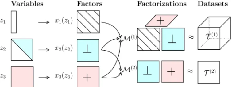
D. A Link Between Datasets as a New Form of Diversity As explained in Section III-C, if all datasets share the same underlying factorization model, and in addition, admit a (multi-) linear relationship, then it may be possible to use a single matrix or tensor decomposition in order to perform data fusion. This assumption may be challenged in various scenarios. An obvious conflict arises when datasets are given in different types of physical units. A technical difficulty is when datasets are stacked in arrays of different orders, such as matrices vs. higher-order arrays. Further examples are datasets with different latent models, different types of uncertainty, or when not all factors or latent variables are shared by all datasets. In such cases, we say that datasets are heterogeneous [8]. While each of these complicating factors may be accommodated by preprocessing the datasets such that they all comply, e.g., by normalizing, realigning, interpolating, up- or down-sampling, using features, or reducing dimensions, these procedures have the risk of being lossy in various respects (for further discussion on complicating factors in data fusion, see Section IV). For these reasons, more elaborate models that allow heterogeneous datasets to remain in their most explanatory form and still perform true data fusion, i.e., in the sense of Definition I.2 and Section V-A, have been devised.
In the following, we discuss data fusion approaches that go beyond single matrix or tensor factorization. Our emphasis is on demonstrating how the concepts of true data fusion allow pushing even further the limits of extracting knowledge from data that were summarized in Section III-C2. We show how these properties are carried over to more elaborate data fusion models and how they can be reinforced into stronger properties that cannot be achieved using single-set single-modal data. In particular, (i) allowing more relaxed uniqueness conditions that admit more challenging scenarios: for example, more relaxed assumptions on the underlying factors, and the ability to resolve more latent variables (low-rank terms) in each dataset, and (ii) terms that are shared across datasets enjoy the same permutation at all datasets. This obviates the need for an additional step of identifying the arbitrarily-ordered outputs of each individual decomposition and matching them, a task that generally cannot be accomplished without additional information, in a blind or data-driven context. Fixing the permutation reduces the number of degrees of freedom and thus enhances performance and interpretability. The following examples illustrate these points.
Example III-D.1: Coupled Independent Component Anal-ysis. Consider the ICA problem (6). It is well-known that statistically independent real-valued Gaussian processes with independent and identically distributed (i.i.d.) samples, mixed by an invertible A, cannot be blindly separated based on their observations x(t) alone [71], [107]. If several such datasets are considered simultaneously, however, without changing the model within each mixture, but allowing statistical dependence across datasets, then a unique and identifiable solution to all these mixtures, up to unavoidable scale and permutation ambiguities, exists [82]. This model, when not restricted to Gaussian i.i.d. samples, is known as independent vector
analysis (IVA) [82], [108], [109] and can be solved using second-order statistics (SOS) alone [110], [111].
IVA was originally proposed to separate convolutive mix-tures of audio signals [108], [109]. In the frequency do-main, this amounts (approximately) to resolving M ICA mixtures (6),
x(m)(t) = A(m)s(m)(t) , t = 1, . . . , T , (11) where the M matrices A(m), m = 1, . . . , M , are generally different (in this context, t denotes samples in the frequency domain and m are the frequency bins). For simplicity, we assume that both x(m)(t) and s(m)(t) are I
× 1. When each mixture (11) is solved separately, it is associated with an individual permutation matrix P(m). It is clear that proper separation and reconstruction of the I audio signals cannot be achieved if the elements of the same source at different frequency bins are not properly matched. The key point in IVA w.r.t. a collection of ICA is that it exploits statistical dependence among latent sources that belong to different mixtures, as illustrated in Figure 1. Under certain conditions, the IVA framework provides a single R×R permutation matrix P(m)= P that applies to all the involved mixtures [82], [109]. The ability of IVA to obviate the need to match the outputs of M separate ICA soon turned out useful far beyond convolutive mixtures: it has since been applied to fMRI group data analysis [112], [113], multimodal fusion of several brain-imaging modalities [114], and the analysis of temporal dynamic changes [115]. IVA extends CCA [1] and its multi-set extension (MCCA) [3], which have both been widely used for fusion [31], [36], [58], [116]–[118], to the case where not only second-order statistics but all-order statistics are taken into account [82]. Recently, a generalization of IVA that allows decomposition into terms of rank larger than one has been proposed [119]–[121]. In addition, since IVA is a generalization of ICA, it readily accommodates additional types of diversity such as coloured (i.e., non-spectrally-flat) or non-stationary sources [111], [122] (recall SectionIII-C1). Identifiability analysis of the multiple types of diversity in IVA is given in [82], [123]. It should be noted that the uniqueness results for coupled CPD [90] (ExampleIII-D.2) require at least one tensor of order larger than two in the coupled set and thus they cannot be applied to IVA.
A(M ) ⎡ ⎢ ⎢ ⎢ ⎢ ⎣ x(M )1 x(M )2 .. . x(M )I ⎤ ⎥ ⎥ ⎥ ⎥ ⎦ s(M ) s(m) s(1) x(1) = ⎡ ⎢ ⎢ ⎢ ⎢ ⎣ x(m)1 x(m)2 .. . x(m)I ⎤ ⎥ ⎥ ⎥ ⎥ ⎦ ⎡ ⎢ ⎢ ⎢ ⎢ ⎣ x(1)1 x(1)2 .. . x(1)I ⎤ ⎥ ⎥ ⎥ ⎥ ⎦ A(m) A(1) ⎡ ⎢ ⎢ ⎢ ⎢ ⎣ s(m)1 s(m)2 .. . s(m)I ⎤ ⎥ ⎥ ⎥ ⎥ ⎦ ⎡ ⎢ ⎢ ⎢ ⎢ ⎣ s(1)1 s(1)2 .. . s(1)I ⎤ ⎥ ⎥ ⎥ ⎥ ⎦ ⎡ ⎢ ⎢ ⎢ ⎢ ⎣ s(M )1 s(M )2 .. . s(M )I ⎤ ⎥ ⎥ ⎥ ⎥ ⎦ x(m) x(M )
dependent
statistically
statistically dependent
Fig. 1: Diagram of the IVA model. Figure reproduced from [116, Figure 1].
Example III-D.2: Coupled Tensor Decompositions. In mul-tilinear algebra, an ongoing endeavour is to obtain uniqueness conditions on a tensor decomposition [67], [88], [92]–[97]. The goal is to derive bounds that are as relaxed as possible on the largest R that still satisfies essential uniqueness (9). As an example, two necessary conditions for the essential uniqueness of the CPD of a third-order tensor (8) are that
(A B) , (C A) and (B C) have full column rank,
and min(kA, kB, kC)≥ 2 (12)
(e.g., [72], [92]) where denotes the column-wise Khatri-Rao product and kAis the Kruskal-rank of matrix A, equal to the
largest integer kAsuch that every subset of kAcolumns of A
is linearly independent [67].
Consider now M third-order tensorsX(m) ∈ CIm×Jm×K, m = 1, . . . , M , with the same factorization as (8), that are coupled by sharing one factor,
X(m)= R
X
r=1
a(m)r ◦ b(m)r ◦ cr (13)
where the factor matrices of the mth tensor are A(m) = [a(m)1 , . . . , a (m) R ] ∈ C Im×R, B(m) = [b(m) 1 , . . . , b (m) R ] ∈
CJm×R, C= [c, . . . , cR]∈ CK×R. The coupled rank of the
set{X(m)} is defined as the minimal number of rank-1 terms a(m)r ◦b(m)r ◦crthat yield{X(m)} in a linear combination [90].
If the coupled rank of {X(m)} is R, then (13) is called the coupled CPD of {X(m)}. It has recently been shown that the coupled CPD may be unique even if conditions (12) are violated such that none of the individual CPDs in (13) is unique [90].
This fundamental result extends to more elaborate scenarios. Uniqueness can be further improved if the order of (at least one of) the involved tensors increases [90]. This is analogous to the previously-mentioned result (SectionIII-C2) for a single tensor, that increasing its order N relaxes the bound on R [57], [91]. Adding assumptions such as individual uniqueness of one of the involved CPDs, full column rank of the shared factor C, or a specific structure such as a Vandermonde matrix, also reinforces the uniqueness of the whole decomposition [90], [124]. Finally, all these results can be extended to more elaborate tensor decompositions that are not limited to rank-1 terms [90] .
Another benefit from coupling is that it helps relax the permutation ambiguity. Coupled tensor decompositions have a unique arbitrary permutation matrix in a manner that extends single-tensor results (9) [125, Section III.A] [90]. Conse-quently, the low-rank terms that are shared by all the coupled tensors automatically have the same ordering at the output of the algorithm.
Linked-mode PARAFAC in which two or more third-order tensors share a mode has first been suggested in [126, p. 281]. The idea was extended to the case of arrays of different orders (one of them must be three-way or higher) in [69, Section 5.1.1]. Coupled tensor decompositions have already proven useful in telecommunications [125], multidimensional harmonic retrieval [124], chemometrics and psychometrics [8], [99], and more. See Figure2afor an example in metabolomics.
spectra Samples Metabolites Excita tion Retention spectra LC-MS Mass Emission Metabolites NMR time spectra TLC-MS XEEM ZNMR YGC-MS (a) (b)
Fig. 2: Illustration of different types of coupling between matrices and third-order tensors. (a) Linked-mode matrices and tensors in metabolomics. Datasets represent four different acquisition methods. All datasets share the same “samples” mode. Figure reproduced from [127]. (b) Arrays (in this case, third-order tensors) may be coupled in different modes and also via only part of a mode. In addition, linked arrays may be regarded as elements in a larger volume (the red cube), in which certain data points are missing. Figure reproduced from [69, Figure 3].
Linked-mode analysis has also been proposed as a means to represent missing values: each tensor is a dataset that by itself is complete, but as a whole, each dataset has only partial information w.r.t. a larger array in which all these datasets are enclosed. This idea is accompanied by a more flexible coupling design where more than one mode may be shared between two tensors and the coupling may even involve only parts of modes, i.e., shared (sub) factors [69, Section 5.1.2]. Figure2b
illustrates this idea. Missing values are further discussed in ChallengeIV-B.4.
We now summarize Examples III-D.1andIII-D.2. In Sec-tion III-C, we have shown that both ICA and PARAFAC can provide sufficient diversity to overcome the indeterminacy problem inherent to FA. We then extended our discussion to jointly analysing M such problems: M×ICA−−−−→ IVA (Ex-joint pdf ample III-D.1) and M×PARAFAC−−−−−−−→ coupled CPDshared factor (Example III-D.2). We have shown that by properly defining a link between datasets, we can extend and reinforce unique-ness and identifiability beyond those obtained by individual analysis, up to the point of establishing uniqueness of oth-erwise non-unique scenarios. In PARAFAC, mixtures share certain factors, whereas in IVA, each mixture has its own individual parameters and the link is via statistical dependence between certain variables. Next, we have shown that all these models are flexible in the sense that they can easily be fine-tuned and modified in multiple ways, in order to better fit various real-life data. More specifically, they readily admit
various types of diversity. A first generalization of these basic models is by relaxing the assumptions within each decomposition: allowing statistical dependence between latent sources of the same mixture in ICA (resp. IVA) leads to independent subspace analysis (ISA) [128]–[132] (resp. joint independent subspace analysis (JISA) [119]–[121]) as well as other BSS models [133], [134]. Relaxing the sum-of-rank-1-terms constraint in PARAFAC leads to more flexible tensor decompositions such as Tucker [6], [7], block term decomposition (BTD) [135], three-way decomposition into directional components (DEDICOM) [136], and others [137]. A second generalization is by combining several types of constraints and assumptions: for example, PARAFAC may be combined with statistical independence [104], [138], non-negativity, sparsity, as well as structure of the latent factors: Vandermonde [72]–[75], Toeplitz [76], among others [16], [65], [106], [139]. A third generalization is increasing the number of types of observational diversity by increasing the tensor order [57], [91]. A fourth is by linking datasets, leading to various coupled models, as explained in this section. When all these types of generalizations are taken into account, one obtains very general data fusion frameworks such as structured data fusion (SDF) [16], coupled matrix and tensor factor-ization (CMTF) [99], linked multiway component analysis (LMWCA) [65], and others [140]–[142]. These generaliza-tions, and many more, are further discussed in Section V. In all cases, the link between underlying factors at different modalities helps not only to enhance uniqueness but also to enable the same ordering for all decompositions, thus further enhancing performance, identifiability, and interpretability. E. Conclusion: A Link Between Datasets is Indeed a New Form of Diversity
The strength of IVA and coupled CPD over a set of unlinked factorizations lies in their ability to exploit commonalities among datasets. In IVA, it is the statistical dependence of sources across mixtures; in coupled CPD, it is the shared factors. In both scenarios, the links themselves are new types of information: the fact that datasets are linked, that elements in different datasets are related (or not), and the nature of these interactions, bring new types of constraints into the system that allow to reduce the number of degrees of freedom and thus enhance uniqueness, performance, interpretability, and robustness, among others. On top of that, the links among the datasets allow desired properties within one dataset to propagate to the ensemble and enhance the properties of the whole decomposition [16]. This is a concrete mathematical manifestation of the raison d’ˆetre of data fusion that we have mentioned in Section II, implying that [11, Section 9] [82], [143]
An ensemble of datasets is “more than the sum of its parts” in the sense that it contains precious information that is lost if these relations are ignored.
The models that we have just presented allow multiple datasets to inform each other and interact, as formulated in
![Fig. 1: Diagram of the IVA model. Figure reproduced from [116, Figure 1].](https://thumb-eu.123doks.com/thumbv2/123doknet/14429063.514824/12.918.75.453.855.1055/fig-diagram-iva-model-figure-reproduced-figure.webp)