Communications Biophysics

Prof. W. A. Rosenblith Dr. R. D. Hall J. W. Davis Prof. M. Eden Dr. N. Y-S. Kiang$ J. L. Hall II Prof. M. H. Goldstein, Jr. A. R. Mllertt J. G. Krishnayya Prof. W. T. Peake Dr. T. T. Sandel** R. G. Mark Prof. H. Putnam Dr. N. S. Sutherland Ingrid Moller Prof. W. M. Siebert Dr. D. C. Teas C. E. Molnar*** Dr. A. E. Albert Dr. Eda Berger Vidale D. F. O'Brien Dr. J. S. Barlowt Dr. T. Watanabe R. R. Pfeiffer Dr. M. A. B. Brazierl Aurice V. Albert C. E. Robinson

W. A. Clark, Jr.** J. Allen E. N. Robinson

Dr. B. G. Farley** R. M. Brown R. W. Rodieck

Margaret Z. Freeman W. H. Calvin G. Svihula

Dr. G. L. Gerstein R. R. Capranica T. F. Weiss A. H. Crist

RESEARCH OBJECTIVES

During the past year publications by members of this group have ranged from certain aspects of applied mathematics1- 4 to certain problems of instrumentation5; most of our work has, however, been experimental in character and has reflected our predom-inant concern with those aspects of the electrical activity of the nervous system which relate to sensory function.

A large number of papers have dealt with the application of computer techniques to analytical studies of neuroelectric activity. Six of these papers are part of a forth-coming special supplement to the Journal of Electroencephalography and Clinical Neuro-physiology in which the proceedings of a conference organized by Professor M. A. B. Brazier at the Brain Research Institute of the University of California at Los Angeles is summarized. 1 0

11-20

Several studies of responses from the auditory and visual systems have been reported. In some of these papers a particular effort has been made to use the tech-niques that we have developed in order to examine those aspects of electrical responses that are peculiarly sensitive to an organism's physiological macrostate. A sustained

effort is already being made to study sensory discrimination in a given organism by means of compatible electrophysiological and behavioral techniques; during the coming year the first findings of this research should be reported.

Analyses of a variety of biologically significant patterns continue to concern mem-21-24

bers of this group _{; some of the papers already referred to could have been put}

This work was supported in part by the National Science Foundation (Grant G-16526 and Grant G-7364); in part by the National Institutes of Health (Grant MP-4737); and in part by the U.S. Air Force (Electronic Systems Division) under Contract AF19(604)-4112.

TResearch Associate in Communication Sciences from the Neurophysiological Laboratory of the Neurology Service of the Massachusetts General Hospital.

Visiting Professor in Communication Sciences from the Brain Research Institute, University of California at Los Angeles.

Staff Member, Lincoln Laboratory, M.I.T.

ttVisitor from the Speech Transmission Laboratory, Royal Institute of Technology, Stockholm, Sweden. "Also at the Massachusetts Eye and Ear Infirmary.

into this category.

Notable progress in research that deals with the behavior of networks of neuronlike

elements is reflected in two papers.25-26

Our close and fruitful cooperation with the Eaton Peabody Laboratory for Auditory

Physiology, at the Massachusetts Eye and Ear Infirmary, continues. The laboratory

now constitutes a model experimental facility for whose design Robert M. Brown, and

for whose operation, Alan Crist, are largely responsible. Under the able and inspired

direction of Dr. Nelson Y-S. Kiang, the past year has been characterized by the

accu-mulation of an impressive catalog of the behavior of neurons in the auditory nerve and

in the cochlear nucleus. There is in preparation a highly significant monograph on the

coding of acoustic stimulus characteristics.

The always present preoccupation of electrophysiologists with the physical

charac-teristics of the medium, and with methods of recording them, has been expressed in

27-29

three papers.

Finally, the relation of neuroelectric and behavioral events that are concomitant

with sensory communication have been examined in two other publications.

' 31

W. A. Rosenblith

References

1.

_{M. Eden, On the formalization of handwriting, Proc. Symposia in Applied}

matics, Vol. 12, Structure of Language and Its Mathematical Aspects (American

Mathe-matical Society, New York, 1961), pp. 83-88.

2.

_{M. Eden, A two-dimensional growth process, Fourth Berkeley Symposium on}

Mathematical Statistics (University of California Press, Berkeley, in press).

3.

_{R. W. Rodieck, Methods of Studying Spontaneous Activity, S.M. Thesis,}

Depart-ment of Electrical Engineering, M.I. T., 1961.

4.

_{D. D. Rutstein, M. Eden, and M. P. SchUitzenberger, Report on mathematics}

in medical sciences, New England Journal of Medicine 265, 172-176 (1961 ).

5.

_{M. H. Goldstein, Jr. and L. Nicotra, Spectral analyzer for EEG, EEG Clin.}

Neurophysiol. 13, 475-477 (1961).

6.

_{N. Y-S. Kiang, The use of computers in studies of auditory neurophysiology,}

Trans. Amer. Acad. Opthalmol. Otolaryngol. 65, 735-747 (1961).

7.

_{M. A. B. Brazier, Detection of evoked responses, Methods in Medical Research,}

edited by J. H. Quastel (Yearbook Medical Publishers, Chicage, 1961), pp. 423-432.

8.

_{M. A. B. Brazier, Editor, Conference on Computer Techniques in EEG Analysis}

(Elsevier Publishing Company, Amsterdam, in press); included are the following papers:

J. S. Barlow, Correlation techniques in EEG analysis;

W. A. Clark, Jr., Digital averaging techniques;

B. Farley, Recognition of patterns in the EEG;

G. L. Gerstein, Neuron firing patterns and the slow potentials;

M. H. Goldstein, Jr., Averaging techniques applied to evoked responses; and

W. A. Rosenblith, Commentary.

9.

B. G. Farley, L. S. Frishkopf, W. A. Clark, Jr., and J. T. Gilmore,

Com-puter techniques for the study of patterns in the EEG, Trans. IRE, PGME (in press).

10.

_{Publication of the teaching materials used in the special, intensive course on}

"Computer Techniques for Biological Scientists," is not contemplated at this time; this

course, which was sponsored by the National Science Foundation, was organized during

the summer of 1961, and taught by a committee composed of T. T. Sandel (Chairman),

J. B. Dennis, W. M. Siebert, W. A. Clark, Jr., and M. Eden.

11. M. A. B. Brazier, Paired sensory modality stimulation studied by computer analysis, Pavlovian Conference, Ann. New York Acad. Sci. 93, Art. 3, 1054-1063 (1961).

12. M. A. B. Brazier, Keith F. Killam, and A. James Hance, The reactivity of the nervous system in the light of the past history of the organism, Sensory

Communi-cation, edited by W. A. Rosenblith (The M.I.T. Press, Cambridge, Mass., and John Wiley and Sons, Inc., New York, 1961), pp. 699-716.

13. G. L. Gerstein, Firing patterns of neurons in auditory cortex, Brain and Behavior Conference (Brain Research Institute, U. C.L.A., February 1961, in press).

14. N. Y-S. Kiang and T. T. Sandel, Off-responses from the auditory cortex of unanesthetized cats, Arch. Ital. Biol. (Pisa) 99, 12 1-134 (1961).

15. T. T. Sandel and N. Y-S. Kiang, Off-responses from the auditory cortex of anesthetized cats: effects of stimulus parameters, Arch. Ital. Biol. (Pisa) 99, 105-120 (1961).

16. N. Y-S. Kiang, J. H. Neame, and Louise F. Clark, Evoked cortical activity from auditory cortex in anesthetized and unanesthetized cats, Science 133, 1927-1928 (1961).

17. A. Arduini and M. H. Goldstein, Jr., Enhancement of cortical responses to shocks delivered to lateral geniculate body: Localization and mechanism of the effects, Arch. Ital. Biol. (Pisa) (in press).

18. N. Y-S. Kiang, M. H. Goldstein, Jr., and W. T. Peake, Temporal coding of neural responses to acoustic stimuli, Trans. IRE, PGIT (in press).

19. W. T. Peake and N. Y-S. Kiang, Cochlear responses to condensation and rare-faction clicks, Biophys. J. (in press).

20. D. C. Teas and N. Y-S. Kiang, Evoked cortical responses as a function of 'state' variables, Quarterly Progress Report No. 59, Research Laboratory of Elec-tronics, M.I.T., October 15, 1961, pp. 171-176.

21. C. F. Ehert and J. S. Barlow, Toward a realistic model of a biological period-measuring mechanism, Cold Spring Harbor Symposia on Quantitative Biology, XXV,

Biological Clocks (Long Island Biological Association, New York, 196 1); see also Discussion, pp. 54, 85, 86, 196.

22. M. Eden and M. Halle, A characterization of cursive writing, Information Theory, edited by C. Cherry (Butterworths Scientific Publications, London, in press).

23. J. S. Barlow, A phase-comparator model for the diurnal rhythm of emergence of Drosophila, Ann. New York Acad. Sci. (in press).

24. S. L. Levine, The Electroencephalogram of Identical Twins, S. M. Thesis, Department of Electrical Engineering, M.I. T., 1961.

25. B. G. Farley, Simulation of nerve nets, Fed. Proc. (in press).

26. B. G. Farley and W. A. Clark, Activity in networks on neuron-like elements, Information Theory, edited by C. Cherry (Butterworths Scientific Publications, London,

in press).

27. M. A. B. Brazier, Electrical fields in a conducting medium, Methods in Medi-cal Research, edited by J. H. Quastel (Yearbook MediMedi-cal Publishers, Chicago, 1961) pp. 416-423.

28. M. A. B. Brazier, Recordings from large electrodes, Methods in Medical Research, edited by J. H. Quastel (Yearbook Medical Publishers, Chicago, 1961), pp. 423-432.

29. C. D. Geisler and G. L. Gerstein, The surface EEG in relation to its sources, EEG Clin. Neurophysiol. (in press).

30. W. A. Rosenblith and Eda Berger Vidale, A quantitative view of neuroelectric events in relation to sensory communication, Psychology: A Study of a Science, Vol. 4, edited by Sigmund Koch (McGraw-Hill Publishing CompanNew- ork, 1962), pp. 334-379.

31. _{W. A. Rosenblith, Editor's Comment, Sensory Communication (The M.I.T.} Press, Cambridge, Mass., and John Wiley and Sons, Inc., New York, 1961), Chapter 40, pp. 815-826.

A. _{MODELS FOR THE DYNAMIC BEHAVIOR OF THE COCHLEAR PARTITION} The hydromechanical action of the inner ear plays an important role in almost every theory of audition, and has consequently long been a popular subject for speculation and investigation. _{The recently celebrated direct observations by George von Bdk6syl-} 8 _of the motion of the cochlear partition put an end to most of the speculation and leave little room for doubt, at least about the general nature of cochlear dynamics. But von Bk4sy's reported results provide only somewhat spotty coverage (particularly with respect to phase characteristics) of low- and medium-frequency response in the middle and apical turns. _{The difficult nature of von B6k6sy's experiments has apparently discouraged}

direct extension of his work; we are left with such deductions as we can make from interpolation and extrapolation, from theory, and from indirect electrophysiological evidence.

The present study is primarily an empirical attempt to extend and complete von Bk~6sy's observations, and was undertaken as part of a continuing effort to under-stand certain psychophysical phenomena. _{It differs from the similar (and similarly} motivated) work of Flanagan9, 10 in two respects:

a. _{We are as much interested in studying the functional structure,} interrelation-ships, and internal consistency of von Bk6sy's observations, as we are in trying to fit the data accurately with specific analytical functions.

b. _{Such analytical representations as we shall give explicitly have been constrained} by a requirement of extreme simplicity and workability, so as to hamper least the psychophysical analyses for which they are intended. In particular, we have seen no reason to limit our search to rational functions of frequency.

1. Von Bk6sy's Observations

We assume that the behavior of the cochlear system would be adequately described for our purposes by giving the volume displacement of the cochlear partition (in cc/mm) of each point, x (in centimeters measured from the stapes), at each time, t (in seconds), in response to an arbitrary dynamic volume displacement (in cubic centimeters) of the stapes. Since the evidence supports the further assump-tions that the cochlear system is - at least for small displacements - both linear and

(essentially) time-invariant, it is sufficient to give both the amplitude and phase of the sinusoidal response at each point, x, to a sinusoidal stimulus of the stapes at an arbi-trary frequency, f, (in cps). Symbolically we can represent this stimulus-response relationship by the complex function F(f, x), which is to be interpreted as implying that, if the volume displacement of the stapes is A cos [Zrft + 6], then the volume displacement of any point on the partition is given by

Re I F(f, x)Aej[ZTft+ ]1

where Re [

]

[

The measurement of a reasonably smooth function of two variables is usually most easily carried out by fixing one variable and determining the behavior of the function with respect to the other variable. This was the scheme adopted by von Bk6sy. His

1-8

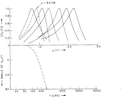
principal reported results are shown in Figs. XXVI-1 - XXVI-4 (the scales of Figs. XXVI-1 and XXVI-2 are rather unconventional as we shall explain). Figure XXVI-1 is, in our notation, a plot of the magnitude of

F(f, x) = H x(f)

(1)

SF[fmax(x),

x

considered as a function of f for various fixed x. Two sets of data are shown; the later data2 _{consist of only one curve, but the corresponding value of x and of the phase} angle of F(f, x) are given, whereas neither the phase nor the position are available for the earlier results.3 Similarly the curves of Fig. XXVI-2 are plots of the magnitude and phase of

F(f, x)

=

Gf(x)

(2)

F[f, Xmax(f)]

_I

considered as functions of x for fixed f. Again, two sets of data are shown. The 1943 set4 _{covers a relatively wide range of frequencies, but no corresponding} phase meas-urements were made. The 1947 results5 include phase measurements, but data are given only for quite low frequencies. It is obvious from Fig. XXVI-2 that although these two sets of curves are qualitatively similar they are quantitatively quite different - the

spread along the partition of the response to a given frequency is perhaps twice as wide for the earlier observations as for the later.

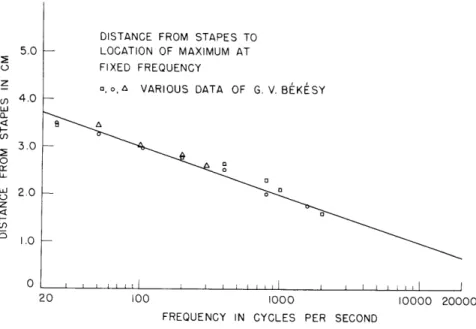
Figure XXVI-3 is a "cochlear map" - a plot of x (f). Three sets of points are

6

max

shown, one from 1942 measurements 6

of this function alone and the others from the peak locations of Fig. XXVI-2. It is important, at least in principle, to observe that we should not necessarily expect to get the same relationship between x and f if we seek to determine the frequency that maximally stimulates a given spot rather than

0 10 2.0 3.0 \ 0\ D

27r-1

Fig. XXVI-1. Frequency responses for various positions along the cochlear partition. Solid curves, von B6k6sy (1943); dotted curves, von Bdk6sy (1947). 1600 800 - 200 S o 50 --- BEKESY (1943) - BEKESY (1949) v(x) 4.0 0 Li -5Ir 21r Z 4 x(CM) 0.75 1.0 1.25 1.5 1.75 20 2.5 30 3.5 STAPES

FIXED FREQUENCY

"o, A VARIOUS DATA OF G. V. BEKISY

.0%

20 100 1000

FREQUENCY IN CYCLES PER SECOND

10000 20000

Fig. XXVI-3.

S I I I IL l I

I

Fig. XXVI-4.

Amplitude factor (after von B6k6sy, 1947).

50 100

(as von B6k6sy did) to locate the position of maximum response to a given frequency.

The first, fmax(x), is the solution of

a IF(f, x)

f

0,

(3)

whereas the second, xmax (f), is the solution of

a F(f, x)

= 0.

(4)

ax

There would not seem to be any special experimental difficulty in determining fmax()

rather than xmax(f) (position labels for the curves of Fig. XXVI-1, if available, would

permit construction of such a curve), and indeed some indirect methods of making

coch-lear maps yield one function and some the other. Thus the locations of lesions in the

basilar membrane which are produced by intense stimulation should give Xmax(f),

where-as the mewhere-asurement of the frequency at which fixed damage causes maximum hearing

loss presumably relates to f max(x).

It is probable that experimental difficulties and

differences between individuals and species would preclude observation of any small

discrepancy between

max (f) and f max(x), but a large difference would certainly have

been noticed by von B6k6sy if it were present. The absence of such a large effect

-

at

least at low and medium frequencies

-

is of considerable importance to our study.

Von Bk~6sy's results, as in Figs. XXVI-1 and XXVI-2, are characteristically plotted

as "relative amplitudes." To determine F(f, x) from these results, it would be

neces-sary to be given separately the amplitude factors

h(x) = F[fmax(x), ]x (5)

and/or

g(f) = F[f, xmax(f)] . (6)

These are, of course, different functions; there is, at least formally, no reason to

suppose that they are related in any simple way such as g(f)

=

h[xmax(f)]. In this respect

the one amplitude-factor plot

given by von B6k6sy (Fig. XXVI-4) is somewhat

con-fusing.

From von B&k6sy's description, Fig. XXVI-4 is based on the same data as the

1943 curves of Fig. XXVI-1, and is the volume displacement per millimeter at a given

point on the partition for a unit volume displacement of the stapes at the frequency to

which the given point is maximally sensitive; that is, Fig. XXVI-4 is a plot of h(x). But

the abscissa of the curve is frequency.

Apparently what is really being plotted is

h[xmax(f)], with xmax(f) given by some unspecified cochlear map.

However, it seems

likely that the difference between g(f) and h[xmax(f)] over at least the frequency region

considered is not likely to be very large or again von B6k6sy could hardly have failed

to detect it. We shall see shortly that perhaps the best evidence that this is indeed the case is provided by the data of Fig. XXVI-4 itself, which show that the maximum ampli-tude is only approximately 4 times greater at a point 2. 0 cm from the stapes than it is

at the helicotrema. As von B6k6sy points out this is "relatively flat," at least when com-pared with the 60 db or more variation in the auditory threshold for the corresponding

frequencies. And it is quite flat enough to make any differences in the low- and medium-frequency region between the plots of xmax (f) and fmax(x) or between g(f) and h[xmax(f)] entirely academic, as we shall see.

2. Deductions and Models

It should be clear from Figs. XXVI-1 - XXVI-4 and the preceding discussion that von B~k6sy does not provide sufficient observations to define F(f, x) directly, even at low frequencies and in the apical region. The most nearly complete description results from the earlier data of Fig. XXVI-1 in combination with the amplitude factor of Fig. XXVI-4, but this provides no phase information, the values of position are not given in Fig. XXVI-1, and the range of frequencies covered is limited. Some addi-tional information - particularly about phase characteristics - could be derived from

Fig. XXVI-2, if the questions of consistency, which arise because the observations were made on separate preparations, could be resolved. To test for consistency as well as to extrapolate in a reasonable way we shall need various principles that we shall now

develop.

First we observe that we must have, for consistent data,

F(f,x) = h(x) Hx(f) = g(f) Gf(x) (7) and hence h(x) = g(f) G(x) (8) Hx(f) or in particular h(x) (x(9)

IHx(f)

for each fixed frequency. If the values of IGf(x) I and IHx(f) I are taken from the curves of Figs. XXVI-1 and XXVI-2 for common values of x and f, then the values of the ratio for each f should form a smooth curve and the curves for various f should be part of one over-all curve, h(x), except for scale factors (which determine g(f)). This procedure is easily carried out for the data of Figs. XXVI-1 and XXVI-2 except for one thing - the values of x to associate with each curve in Fig. XXVI-1 are unknown. If

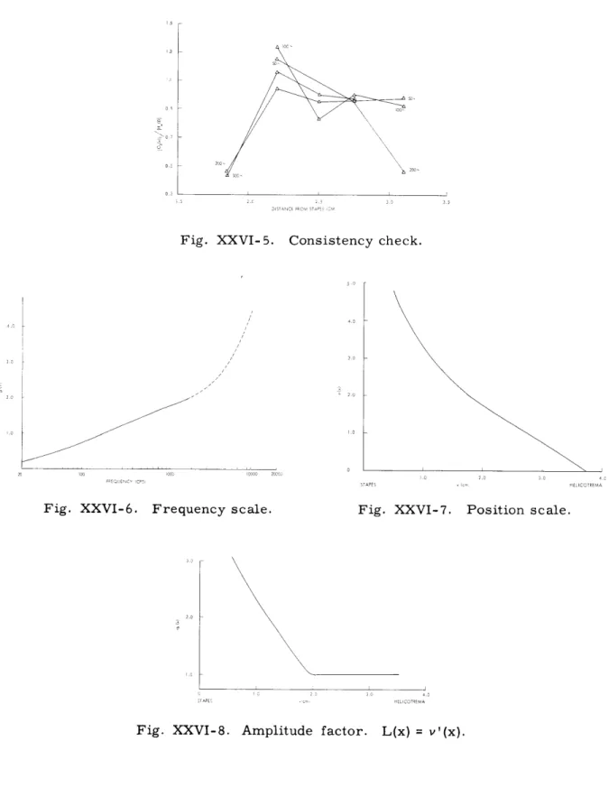
Consistency check.

Fig. XXVI-6. Frequency scale. Fig. XXVI-7. Position scale.

Fig. XXVI-8.

Fig. XXVI- 5.

we assume, tentatively, that max (f) and f max(x) determine the same curve so that the parameter values for Fig. XXVI-1 can be determined from Fig. XXVI-3, it is easy to show (see Fig. XXVI-5) that the curves of Fig. XXVI-1 and the 1947 curves of Fig. XXVI-2 are astonishingly consistent and yield h(x) = g(f)

=

and low frequencies - a result that we consider not inconsistent with the "relatively flat" amplitude factor of Fig. XXVI-4. We have, however, been unable to find any way

of assigning positions to the curves of Fig. XXVI-1 which will yield consistency with the 1943 curves of Fig. XXVI-Z.

There is, moreover, another and independent way in which we can arrive at similar conclusions to those given above. This procedure depends on two observations - one an induction from von Bk6sy's data and the other of a more theoretical nature. Von B6kosy observed3 in his paper of 1943 that, when plotted on a logarithmic frequency scale, the curves of Fig. XXVI-1 "could be brought into tolerably good coincidence by parallel displacement along the abscissa" except at low frequencies at which there was a pro-gressive "flattening" or broadening. This "flattening" can be largely eliminated by choosing a low-frequency scale somewhat more compressed than logarithmic (Figs. XXVI-1 and XXVI-6). Von Bk6sy's data are not given for frequencies higher than 2-3 kc, but it is at least plausible that similar performance would continue for higher frequencies; that is, when plotted on an appropriate scale the response curves would be similar except for displacement of their maxima. But of course there is no special reason to assume that the "appropriate scale" is, even approximately, logarith-mic. One series of experiments which both suggests that this extrapolation is reasonable and also provides a possible form for the scale is the electrophysiological observation by Kiang and Watanabe 11 of the tuning curves for first-order single units in the cat. These results suggest that the bandwidths of the response curves continue to increase as the frequency of the maximum increases, but at a less than proportional rate so that a scale somewhat more expanded than logarithmic is required to yield similar curves. The dotted extension of the scale of Fig. XXVI-6 is highly conjectural, of course, but, as we shall see, it is partially checked by a requirement for consistency.

Let us represent the scale that gives displaced but similar response curves (Fig. XXVI-6) by 1(f). Then the assumption that the curves are indeed similar when plotted on this scale is equivalent to assuming that

Hx(f)

=

H[

±(f) -v (x)]

(10)

where IH[y] is a function giving the shape of any one curve and, if we arbitrarily choose the maximum of IH[y]I to occur at y = 0, then v(x) = 4(f) determines the loca-tion of the peaks; that is,

In addition, and tentatively, we are going to make the still stronger assumption that

not just the magnitude curves but also the phase curves

-

when plotted versus 4(f)

-

are

similar except for displacement so that

Hx(f)

H[

(f) - v(x)]

(12)

and

F(f, x) = h(x) H[ L(f) - v(x)] . (13)

There are a number of disturbing features to von B6k6sy's phase curves which make it

somewhat difficult to test this assumption.

In the first place, his curves uniformly

show the phase angle tending to zero as either f or x tends to zero. It seems probable

that this is more an extrapolation than a direct observation, since the amplitudes of

vibration

-

remote from the maximum

-

must have been extremely small. However,

Flanaganl0 has suggested on physical grounds that the phase angle should approach

r/2 radians for low frequencies.

This argument is, essentially, that at frequencies

that are low enough the flow pattern must be principally a streaming through the

helico-trema with the velocity at each point proportional to the velocity at the stapes, that is,

leading by Tr/2 radians the displacement at the stapes.

At these frequencies the

domi-nant pressure effects should, moreover, be due to viscosity, that is, in phase with the

velocity, and the most important property at the partition should be its elasticity, so

that, finally, the displacement at the partition should be in phase with the pressure

dif-ference, and thus lead by

wr/2

radians the displacement at the stapes.

This is a

com-pelling argument

-

it is hard to see how it can fail to be correct at sufficiently low

frequencies.

But at frequencies for which there is substantial motion at the partition there is no

reason why the pressure difference must be more or less in phase with either the

velocity (as Flanagan suggests) or with the displacement at the stapes (as von Bdk6sy

shows).

Still, if the principal pressure drop were across the partition, it is plausible

that the phase relation between pressure difference and stapes displacement might be

almost fixed, independent of frequency, and consequently the phase angle at F(f, x) might

appear to be approaching a constant (not necessarily 0 or w/2) as f tended to zero

(even though ultimately it would have to actually approach rr/2 as the effect of the

heli-cotrema became important).

The presence of the helicotrema is thus a dominant element in Flanagan's argument.

However, von B6kdsy's experiments do not show any obvious effects of the helicotrema

down to frequencies as low as 50 cps, or even lower. These results suggest that the

simplest model

-

adequate perhaps even for relatively low frequencies

-

would be to

imagine the cochlea as being extended indefinitely beyond the apex with a smooth

con-tinuation of the properties that it has in the apex-base region. And for such an extended

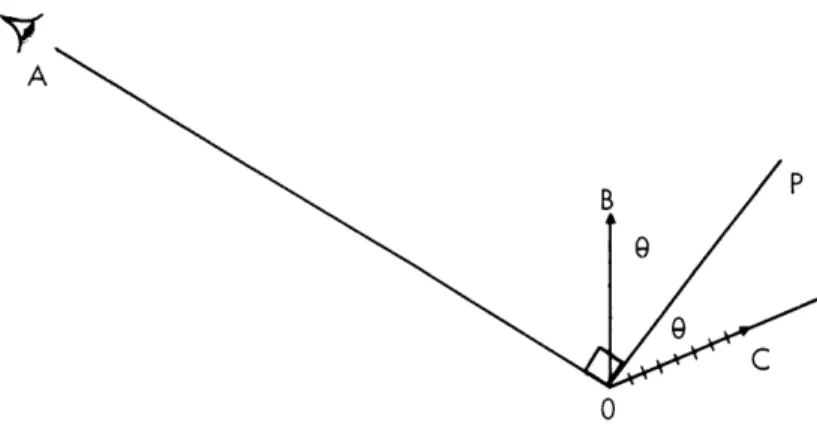
cochlea there is no clear reason why the asymptotic phase angle of F(f, x) need be either 0 or Tr/2.

The concept of an extended cochlea is most useful for theoretical purposes because if we assume incompressible fluids, tissues, and walls, then the volume displacement of the stapes must at every instant be equal to the integrated volume displacement of the partition. This assumption implies an interrelationship between the amplitude and phase of F(f, x), which permits another test for consistency. It also provides an

absolute indication of amplitude which can be checked against the data of von B6kesy. Flanaganl0 has already proposed a different consistency check between the amplitude and phase of F(f, x) which is based on the requirement that F(f, x) must, as a linear system for each x, be both realizable and stable. Such a test is not only somewhat awkward to apply but has the disadvantage that it is highly sensitive to minor changes in even the "tails" of F(f,x), which we certainly can not assume to be accurately known. In contrast, the present test is sensitive primarily to regions in which

F(f, x) is large.

To formulate this test for a sinusoidal drive, from the definition of F(f, x), we have

Re 10

F(f, x) Aej[2lrft+]

dx

=

Re Aej[2

ft+o

(14)

or simply

10 F(f, x) dx = 1. (15)

Here, the factor of 10 comes from the units of F(f, x). Applying this formula to the representation of (13), we have

0 h(x) H((f) -v(x)) dx = 1/10 (16)

J0

which must be true for all values of f. Recalling the significance of v(x) as given by (11) and the shape of 4t(f) as suggested by Fig. XXVI-6, we find that it is reasonable to assume that v(x) is a monotonic decreasing function of x with

v(x) - -oo as x - oc (17a)

and

v(x) - co as x - 0. (17b)

If we make the change of variable,

y =

4(f)

Then (16) becomes

v'(x)j

H(y) dy

=

1/10

(19)

which can only be independent of f if

h(x) ~ v'(x)

.

(20)

Equation 20 is rather intriguing because

it

relates the amplitude factor, h(x), to an

apparently independent quantity derivable from a cochlear map. Actually, we can go

further; if (20) holds, then we know from the properties of cochlear maps that h(x)

will be rather slowly varying compared with

H[4(f) -v(x)]j, so that the maximum of

h(x) H[p(f)- v(x)]j versus x for fixed f will be nearly at the same point as the maximum

of

IH[p(f)-v(x)]j alone, that is, at v(x)

=

4(f).

Or, in other words, the loci of

Xmax(f)

and fmax(x) will be nearly the same, as is observed experimentally.

Furthermore, we

must have, then,

g(f)

=

h[xmax(f)

(2 1)

and

Gf(x)

=

H[

(f)-v(x)]

(22)

so that the curves of G f(x) when plotted against the scale v(x) should be approximately

displaced replicas of the same curve as Hx(f) plotted against 4(f), except that they

would be turned around.

The curve of v(x) in Fig. XXVI-7 has been obtained by

inter-preting the plot of

max

(f) in Fig. XXVI-3 as a plot of 4(f)

=

v(x) with

p(f)

given by

Fig. XXVI-6.

This curve of v(x) has then been used as the scale in Fig. XXVI-2; the

extent to which each set of data

in

Fig. XXVI-2 is

a family of similar curves and the

extent to which the 1947 set, at least, consists of curves similar to those in Fig. XXVI-1

in both magnitude and phase are gratifying checks on our entire procedure.

Finally,

v'(x)

-

h(x) is plotted in Fig. XXVI-8, which shows

that, for large x, h(x) is

approxi-mately constant, as has already been deduced on other grounds.

We thus suggest that von B6kdsy's data may be described, interpolated, and (with

some caution) extrapolated by representing

the sinusoidal response of the partition in the

form

F(f,x)

=

v'(x) H[(f)-v(x)]

(23)

so that only four curves need to be given

-

the scales g(f) and v(x) (or either one of

them and a "cochlear map" that can be interpreted as a plot of 4(f)

=

v(x)), and the

response curve H[y] (which, of course, is complex and hence requires two curves). We

would suggest that p(f) and v(x) might typically look like Figs. XXVI-6 and XXVI-7 and

that H[y] might look like the dotted curve of Fig. XXVI-1 with the origin of the abscissa

moved to the frequency of the peak. (It might be necessary to make minor additions and adjustments to satisfy Eq. 15.) It must be kept in mind, however, that our arguments for (23) are largely empirical. We are unaware of any serious experimental contradic-tions (the assumpcontradic-tions are largely supported by cochlear microphonic data, 1 1 for example), but any curve-fitting model such as this one is completely at the mercy of

new experimental evidence.

3. An Analytical Model

At low and medium frequencies and in the corresponding apical region, k(f) and v(x) (from Figs. XXVI-6 and XXVI-7) can be well approximated by

4(f) = logl0f - 1.25 (24)

and

v(x) = 3.75 -x; v'(x) = -1 (25)

or

4(f) - v(x) = logl0f + x - 5. (26)

The curve p(f) - v(x) = 0 is an excellent fit to the cochlear map of Fig. XXVI-3, as sug-gested by Greenwood.12 For many purposes it would be convenient to have a complete analytical representation for F(f, x) = -H[4(f)-v(x)]. For the application that we have in mind it would be especially valuable if F(f, x) could be easily transformed or inte-grated with respect to either x or f. This fact and the observation that the skirts of H[i(f)-v(x)], if it is considered as a function of f, are rather steep to be represented easily by a rational function, has led us away from the type of approximation selected by Flanagan.10 By a long process of cut-and-try we have arrived at the following func-tional form, which bears a loose relationship to a formula derived by Zwislocki 13 on fundamental grounds: F(f,x) = ko( x) exp-kl(

-x

S

where k is a complex constant, k is its complex conjugate, and k1 and k2 are real

constants to be adjusted to approximate the data and to satisfy (15). F(f, x) as given by (27), is a little different in form from that previously assumed and is not as complicated as it looks. For purposes of manipulation it is desirable to extend the

domain of F(f, x) to include negative frequencies and to arrange that

F(-f, x)

=

F(f, x).

(28)

This accounts for the presence of the second term; for any interesting positive frequency it is so small that we can safely ignore it and obtain

2

5

f

F(f, x) is a function of

-exp

-k

1x

)]

as desired.

The magnitude of F(f, x), from (29), is approximately

F(f,x) kI( f-_) exp -kl I( f

-0 5-x 1 05 - x

which, as may readily be checked, has its maximum at f - 1 5 - x 10 or logl0 f + x - 5 = 0 as required, and I F(f ax, X) = h(x) l ko

independently of x in accordance with (25) and (20). Comparing IF(f, x) / F(fmax' x)I with Figs. XXVI-1 and XXVI-2, we find that the best fit seems to be

k 1

=

(see Figs. XXVI-9 and XXVI-10).

To find k

_o

_2'

0

F(f, x) dx = 1/10

+ (3

j2r)k

5-

f

105-x

10

dy

=

(in 10) y dx, and the integral becomes

) (

-x

1

(31)

(32)

(35)

(36)

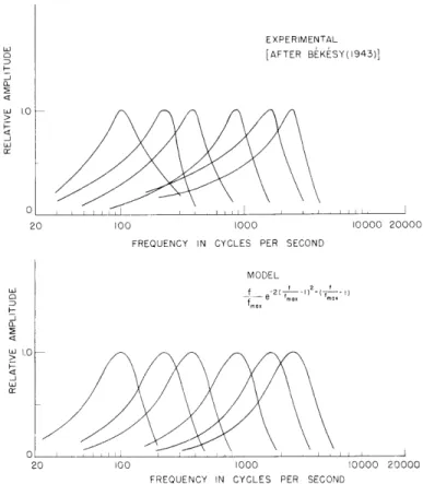
20 100 1000

FREQUENCY IN CYCLES PER SECOND

10000 20000

MODEL

f 21

ef

100 1000 10000 20000

FREQUENCY IN CYCLES PER SECOND

Fig. XXVI-9. Frequency responses for 6 positions along cochlear partition.

z U E LI 0 4 i) o

t

_I

DISTANCE FROM STAPES (CM)

2.0 2.5 3.0 3.5

710

_j

/00

Fig. XXVI- 10.

Volume displacement for various fixed frequencies.

4 ID FJ 4. a

27r-eo 0

i

exp -2y2+ (3-j2 k

)y dy

₍₃₇₎

e(in 10) 10 f

With an error of less than 10 per cent we may extend the lower limit

and evaluate

the integral by completing the square in the exponent to obtain

k 0' (3-jZlTk ₂) 2\ 1 o - exp +

8-

Let

J~o

=

where

is the asymptotic phase angle of F(f, x) as f approaches zero for the extended

cochlea, as already discussed, and Iko is the peak volume displacement per

milli-meter per unit stapes volume displacement and has, from von Bk6sy's data, a value of

cc/mm

the order of 1

cc

From (38),

(rrk2 )2 2

koe

. 162

(40)

and

4-2

where n is any integer. If Ikol is approximately unity, then k

can not be much

out-side the range

1

3

-<k <

2 '2

4'

which implies a change in phase between f

=

0 and the frequency at maximum response

that is between -rr and -3rr/2 radians.

Since von B6k6sy's phase measurements are

quite precise but might be uncertain by multiples at Tr, the most reasonable choice for

cc/mm

Iko

=

1.46

cc

(42)

The resulting response curves, compared with the data of Figs. XXVI-1 and XXVI-2,

are shown in Figs. XXVI-9 and XXVI-10. Multiples of

have been added to von Bk6sy's

phase curves to improve the comparison.

The resulting function representing F(f,x)

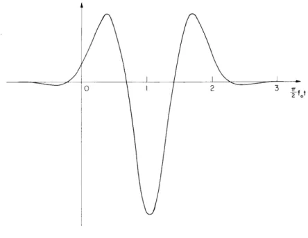
Fig. XXVI-11. Impulse response at point on cochlear partition which responds maximally to frequency fo. (From Model, normalized.)

0- 2

I --

K

DISTANCE FROM STAPES (CM)

Fig. XXVI-12.

Time of propagation of clicks along

cochlear partition.

(Eq. 27) can be transformed exactly to yield the response to an impulsive displacement of the stapes.

1 j2Tr ft -2 2

2r F(f, x) e df = -2. 0 3fmax(x) e (3/4 cos 3 - sin 3 ) (43)

5 - x

(1 fmax)

t

where f max(x) _max = 1 0 and = 7 ₃ - ₂ .max(x Equation 43 is plotted in normalized form in Fig. XXVI-11. The small "tail" extending into the region t < 0 implies that F(f, x) is unrealizable, but this, as we have suggested, is a consequence of the particular form of approximation selected and is not, in our view, very significant.

One final derived quantity is the "travel time for pulses along the cochlear partition." Assuming that the "first deflection" of a given point on the partition as observed by von B6k6sy corresponds to the time of the first maximum in Fig. XXVI-11, we obtain the delay plot of Fig. XXVI- 12 which compares very favorably with his data.8

W. M. Siebert References

1. G. von B6k6sy's papers have been collected in Experiments in Hearing (McGraw-Hill Book Company, Inc., New York, 1960).

2. Ibid., p. 461. 3. Ibid., p. 454. 4. Ibid., p. 448. 5. Ibid., p. 462. 6. Ibid., p. 442. 7. Ibid., p. 455. 8. Ibid., p. 458.

9. J. L. Flanagan, Bell System Tech. J. 39, 1163 (1960). 10. J. L. Flanagan, personal communication, 1961.

11. N. Y-S. Kiang and T. Watanabe, personal communication, (1961) (to be published). 12. I. Tasaki, H. Davis, and J. P. Legouix, J. Acoust. Soc. Am. 24, 502 (1952). 13. D. D. Greenwood, J. Acoust. Soc. Am. 33, 1344 (1960).

14. J. Zwislocki, Acta Oto-laryngol., Supplement 72 (1948).

B. SOME RESULTS OF COMPUTER SIMULATION OF NEURONLIKE NETS 1. Introduction

There exists little understanding of the behavior of neurons interacting in large numbers. It is true, of course, that experimental knowledge of the behavior of the neuron itself and its relationship with others is still incomplete, particularly in the case

of the dendritic tree. However, enough is known so that reasonable guesses can be made as first approximations. With such approximations as hypotheses we would then like to know if the resulting behavior in any way resembles known experimental findings. Unfor-tunately, even the simplest and roughest approximations of this kind lead to systems of

great complexity and nonlinearity. In such cases it is natural to use a computer for aid in the solution of the problem.

The method used in this study has been to construct, in the Lincoln Laboratory's TX-2 computer, a system of neuronlike elements with specified interactions and con-nections. These elements or "cells" and their connections have the following properties. Each element has a definite threshold for incoming excitation below which no action occurs, and above which the element "fires." These thresholds are distributed according to a specified distribution (usually normal) over the elements. When an element fires, its threshold immediately rises effectively to infinity, and then, after a short absolutely refractory period, falls exponentially back (relatively refractory) toward its quiescent value. A short time after firing (the situation is the same for every element) an element transmits excitation to all of the other elements to which it is connected. In the present model all of the connections possess the same effectiveness or "weight." The excitation

is added to any already present at the succeeding cell, after which the excitation sum decays exponentially to zero. If at any time the excitation exceeds the threshold of the succeeding element, that element performs its own firing cycle and transmits its own excitation. During the firing cycle, the element is said to be "active." Note that, in physiological terms, both "spatial" and "temporal" summation are present, and that the

element is "analog," not purely digital. Note also that firing is not forced to be syn-chronous. External stimuli are introduced by instantaneously adding a large value to the excitation function of each stimulated cell.

The present nets have been given a quasi-planar or sheetlike topology, each cell having a probability of connection with its neighbor which depends on radial distance only. This probability distribution is under the control of the experimenter, and he can select beforehand the type of connection pattern that he wishes to try. The nets used in this study have had 1296 elements, arranged in a 36 X 36 array, and the average number

of connections to a cell has varied from 1 to 50, or more.

After the computer program assigns connections according to the desired probabil-ity distribution, and other net parameters are fixed, the operator may choose the ele-ments that are to be stimulated initially by means of a photoelectric device on the TX-2 oscilloscope face that displays the array of cells. The computer then proceeds to cal-culate the resulting activity by using time increments that usually correspond to one-half the absolutely refractory period. Each such time increment actually takes

approxi-mately 1 second in computer time for the 36 X 36 -element networks. Decay-time constants of the relatively refractory period have been in the range of from 0 to 10 times

the absolutely refractory period. Activity is indicated for the experimenter by bright-ening the spots corresponding to fired cells.

2. Tightly Coupled Nets

For qualitative description of observed behaviors, it is convenient to divide the networks roughly into two classes - nets with tightly coupled connections, and loosely coupled nets having relatively long connections. Tightly coupled nets tend to produce well-defined "dense" wave fronts, and the loosely coupled tend to oscil-late diffusely.

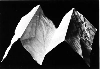
Nets with tightly coupled connections were the subject of a previous paper, 1 so they will be described only briefly here. If each element of the net is connected only with its immediate neighbors, and a single stimulus is given to a few neighboring cells, a "wave" of activity (fired cells) is generally seen to progress away from the site of the stimulus. As long as only one stimulus is given, or if it is repeated at long intervals, the wave fronts form expanding rings much like those formed by a pebble dropped in a pond. No reflections are observed at the edge of the net. Each wave "pushes" before it a precursor of excitation which has not yet fired cells, and furthermore, leaves behind it a "trough" of refractory cells. Thus if waves interact from a rapidly repeating source or from multiple sources, the interaction will be very nonlinear. A rapidly repeating stimulus may produce, not rings, but a very complex "broken" field of wave fronts, which may continue to re-excite itself after the stimulus stops. If multiple stimuli exist, waves of activities may appear which are not produced when the stimuli are given one by one. This behavior can give the effect of inhibition, since the addition of a stim-ulus can cause some cells to stop firing. Many different "modes" of self-excited oscil-lation are possible. A particularly pervasive and striking one consists of one or more continuously rotating spirals. The arms of a spiral maintain such a distance that the refractory trough lies between them.

It has been found possible to obtain a measure of control over the activity by changing the mean threshold of cells by external means. Obviously, if the thresholds in a set of cells are made high enough, no activity can invade it, so that complete inhibition results. Conversely, if thresholds are lower, propagation of activity is made denser and faster. It is therefore possible to exert a control over timing and firing of particular cells or sets of cells. In certain cases the activity circulates repetitively, so that a periodic or nearly periodic firing pattern continues until thresh-olds are changed.

Beurle2 , 3 discussed tightly coupled nets of this general type. He pointed out that in an uncontrolled net, waves of activity tend either to decrease with distance and time or to increase until they become "saturated," that is, activating all of the cells as they pass. We have seen examples of both kinds of behavior.

3. Loosely Coupled Nets

If there are significant numbers of connections that are long enough to reach beyond the refractory trough of a wave, then "backfiring" behind waves can occur. In such a case, the wave fronts become fuzzy, or may not be apparent at all, with activity occurring diffusely over the whole net. The definition of "loosely coupled" thus depends upon tile relative values of connection and refractory trough lengths, which in turn depend on connection delay time and refractory time constants. If the net constants are such that the connections are just long enough for backfiring to take place, the whole net will usually oscillate diffusely after a single stimulus. The oscillation may continue indefinitely, or may sometimes stop spontaneously after a burst of a few or many cycles, particularly if the net is on the edge of oscillating. It is easy to understand this behavior qualitatively. A few cells initially stimulated cause more to fire, which in turn fire others in an increasing sequence. This increase continues until a large proportion of the cells are in a refractory state; firing must then decrease progressively until the refractory cells have recovered, and then the cycle recommences if there is still activity in the net. Thus, if the total number of cells that are firing is plotted as a function of time, a roughly periodic function results. The waveform of the oscillation is not sinusoidal, but is considerably smoother than waveforms usually associated with "relaxation" oscillations.

Allanson4 set up difference equations for a similar net but with completely random interconnections and other simplifications. He was not able to solve the equations because of their nonlinearity, but he was able to predict oscillations and work out some numerical solutions.

There is a number of other features of loosely coupled net behavior which are of considerable interest. Some exist because multiple modes of oscillation are possible. During oscillations activity may be spread diffusely and evenly over the net, and rise and fall more or less in phase everywhere. This "normal" mode gives rise to the large amplitude oscillations just discussed. However, modes in which activity trans-fers from place to place in the net are also possible. Such modes do not show large amplitude fluctuations on total activity-vs-time plots because many cells are always firing. In fact, the total number of cells firing may remain almost constant, and hence very little change in output is observed. Because the cells that will fire at the next instant depend on the particular cells fired at the present instant, as well as past his-tory, the modes are coupled, and activity can transfer from mode to mode. (This lan-guage, borrowed from linear-oscillator terminology, is, of course, only a descriptive analog.) The result of this mode changing upon the total firing-vs-time plot, is that irregular amplitude modulation of the oscillation takes place, but the period remains the same. The net may therefore show irregular "bursts" of rhythmic oscillations,

Fig. XXVI-13.

Network oscillation showing

amplitude-modulated rhythmic burst.

A single

small stimulus was given to start the

oscillation that continues indefinitely

in this manner.

* : .' : c.

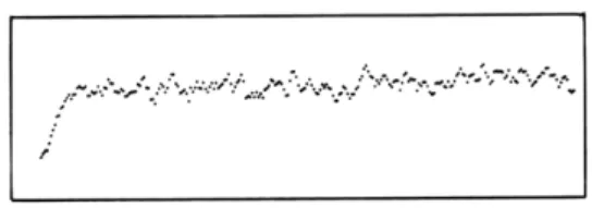
Fig. XXVI-15.

Response of the network shown in

Fig. XXVI-14 when stimulated with a

burst of 14 stimuli at its "resonant"

frequency.

The burst starts a short

time after the initial stimulus. An

expanded time scale is shown in

Fig. XXVI-16 for better time

reso-lution.

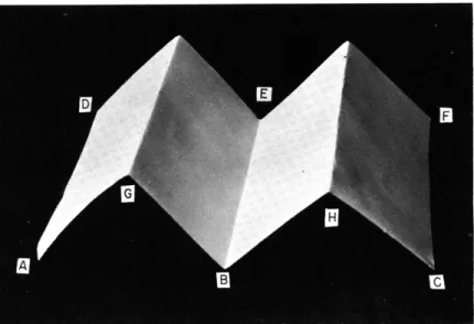
Fig. XXVI-14.

Activity in network without pronounced

rhythmicity. A single stimulus, given

at the beginning of the trace, produced

the initial rise at the left.

Fig. XXVI-16.

First few responses of

Fig. XXVI-15 on an

expanded time scale.

Note "augmenting"

re-sponses.

~'~~ ' ''

' '...

and this behavior continues indefinitely. Figure XXVI-13 shows a short section of such a graph photographed from the output oscilloscope of the TX-2. The total number of cells firing is plotted vertically, and the discrete time instants horizontally.

For any oscillating system, it is of great interest to know what determines the period of the oscillations. In the present case the period is a complex function of refractory time constant, length of connections, and excitatory time constant, and it has not yet been possible to unravel the details. However, it appears that the following explanation is qualitatively correct. The primary determinant of the period is the refractory period itself. This fact can be demonstrated by eliminating the relative refractory period. Then, if the net oscillates in the normal mode, its period is the same as the absolute refractory period. With the exponentially decaying, relative refractory period in effect, the oscillation period ordinarily lies somewhere between the absolutely refractory period and the end of the relative period. However, the oscillation period will not increase indefinitely as the exponential time constant is increased because, as we have seen, the possibility of "backfiring" will eventually disappear, and the net will fail to continue oscillating. Thus, the connections must be lengthened to obtain a longer period. We have not yet studied the effect of transmission delay time, preferring still to keep the model one in which delay time is small compared with the other times. Thus far, we have assumed an excitatory time constant that is much smaller than the refractory period. If this becomes large, it may have the seemingly paradoxical effect of decreasing the period of oscillation because excitation builds up over all of the net and cells begin to fire earlier upon the decay of their relative refractory period.

Our discussion has indicated that the oscillation period is quite independent of net-work size and shape, amplitude of oscillation, and initial stimulus, and partly inde-pendent of the connection lengths and excitation time constant as long as they are not extreme. These predictions are borne out by observation, at least to a first approxi-mation, although it must be kept in mind that these are conclusions from preliminary data. The period is not precisely constant from peak to peak; in fact it may vary 20 per cent or 30 per cent, and the variation of average frequency over a long period of time has yet to be investigated.

The precise course of the activity during oscillation depends on the cells that are initially stimulated, and small differences in inital stimulus or small changes in net parameters cause large differences in activity pattern, or even in the total activity plot after some time. The assumption is, of course, that there is no "noise" in the system in the form of random firing. If noise is present, as it will be in a real system, the oscillation will eventually lose its dependence on initial stimulus just as it would in any oscillating system. Hence the usefulness of this effect in small-difference detection will depend on the amount of noise present, as well as on the method of detection. The same thing is true if some function of activity is used for classification of stimuli. These

matters require further investigation.

We have been discussing networks that are set in oscillation by a single stimulus.

There are also interesting behaviors to be observed if networks (with self-excited

activity already started) are given further stimuli. In the first place, it might be

expected that an oscillating net can be synchronized or "driven" by a repeated stimulus

near its natural period.

This is, in fact, the case, if the stimulus is not too small or

too large. If it is too small, it will do nothing; if it is too large, the first stimulus may

put too many of the cells in a refractory state and stop all activity.

Some nets, if the refractory and excitatory periods are below optimum for normal

oscillations, will produce self-excited activity that shows little or no evidence of

peri-odicity (at least to the naked eye).

The total activity-vs-time plot of one such net is

illustrated in Fig. XXVI-14.

If such a net is stimulated periodically with a diffuse

con-stant stimulus, the average amplitude of the responses after the first few varies with

frequency in a manner somewhat similar to an ordinary resonance curve, with peak

response occurring at a frequency that is determined by the refractory period. The

stimulus must be above a certain threshold for this effect to take place. Furthermore,

at or near the resonant frequency, the first few responses build up, or augment, to a

maximum level, after which the responses may stay more or less constant (especially

with large stimulus on-resonance), or they may wax and wane.

Figure XXVI-15 shows

this in the same net that is illustrated in Fig. XXVI-14.

A stimulus train was started

soon after the net had achieved its normal level of self-excited activity. Note that

although it takes several responses to build up to a maximum, the response in this net

ceases immediately after the response to the last stimulus.

Figure XXVI-16 shows the

first few responses shown in Fig. XXVI-15 which have been expanded in time. At

stimulus frequencies that are multiples or submultiples of the resonant frequency, the

response may synchronize with the stimulus, may "skip" stimuli, or move from one to

another of these modes.

Since the second response of a series may be either larger or

smaller than the first, the size depending on their separation, as indicated by the type

of experiment discussed above, it is of interest to measure the size of the second

response as a function of separation when there are only two stimuli in a "train."

In Fig. XXVI-17 are shown the results for one net.

The amplitude of the second

response relative to the first is plotted as a function of separation.

Each point is an

average of 10 trials to reduce fluctuations introduced by differing initial conditions in

the spontaneously active net.

The dotted part of the curve is not well established,

because of time-resolution limitations of the present calculation. The second response

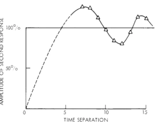
amplitude performs a decreasing oscillation about the amplitude of the first.

Thus the nets produce at least three interesting results upon stimulation which are

related. Their relation may be understood qualitatively as follows.

In general, if a

large group of cells in an active net is stimulated from outside, not all will fire because

z o 100/o z

2

Fig. XXVI-17. Amplitude of response to second stimulus (per cent of first response) as a function of separation of stimuli. The two stimuli were given to a spontaneously active net similar to that shown in Fig. XXVI-14.

many will be refractory. After waiting a proper length of time, those cells fired by the stimulus will have recovered (except for some that may have been refired internally) and, also, those that were refractory at the stimulus time will be available (except for some that may have been refired internally). Thus, if the ratio of stimulated cells to internal average firing rate is large enough, we may expect a second stimulus, given at the proper time, to fire a larger number of cells than the first. The "transient" intro-duced by a stimulus may go through several "cycles," which accounts for the variation of amplitude of a second response with time separation. At the right period, the aug-mentation of response may last for several responses, whereas at other periods, the second and later responses may remain smaller than the first. Therefore a peak of amplitude vs frequency can occur if the first few responses are ignored. The "resonance" phenomenon, augmenting responses, and two-stimulus response variation, can therefore all be viewed as consequences of the refractory properties of the units.

4. Discussion

It is clear that the model has interesting and sometimes unexpected properties even when it is considered solely as an abstract system for study. However, it is also evi-dent that there are qualitative similarities between the behavior of the model and some experimental findings in electrophysiology. One's attention is particularly drawn to the oscillatory and response behavior of the loosely coupled nets which is reminiscent of several well-known "slow-wave" phenomena, notably the EEG, and the "recruiting" and "augmenting" responses. That "reverberating" refractory mechanisms of the kind studied here might account for some of these phenomena is, of course, not a new idea in physiology. Related ideas have been suggested, for example, by Verzeano, Lindsley, and Magoun.5 (See also Walter 6 for a review.) Allanson4 also suggested that oscillations

of the diffuse type might be related to the EEG. The fact that the nets can exhibit burstlike rhythmic activity and irregular waves, as well as simple oscillations, makes the resemblance even more striking. The synchronizing or "driving" phenomenon may perhaps also be cited as an additional similarity. It is somewhat difficult to separate

"driving" behavior from response to stimulation, and this requires more study. This is, of course, also true of EEG driving behavior.

Similarities to aspects of the "augmenting" and "recruiting" responses may also be seen by reference particularly to Jasper, and to Purpura and Housepian.8 The increase of the first few responses and the sudden cessation of response can occur in both net and electrophysiological experiments. The same is true of waxing and waning of the response under certain conditions. Rosenblith9 and Freemanl 0 have observed physiological "resonance" curves of response amplitude. It is interesting that aug-menting and two-stimulus oscillations were also present in the same systems. The two-stimulus experiment is analogous to the "two-click" experiments that have been previously studied in physiological acoustics. Rosenzweig and Rosenblith11 observed oscillations of the cortical response to the second click of a two-click stimulus as a function of time separation.

In summary, at least the following similarities between the loosely coupled networks and electrophysiological phenomena have been observed:

(a) Oscillations with burstlike amplitude modulation, (b) "Synchronization" of oscillations,

(c) "Resonance" of response amplitude,

(d) Augmentation of responses - sometimes with amplitude modulation, and (e) Oscillatory variation of the second of two responses vs time separation.

Some effects observed on stimulation at multiples and submultiples of the resonant frequency may be common to both model and experiment. These similarities are still, for the most part, qualitative, and a great deal more theoretical and experimental work will be required before it can be determined whether systems with the properties of the model exist (among many others) in the brain, or if the similarities are merely remarkable coincidences.

B. G. Farley

References

1. B. G. Farley and W. A. Clark, Jr., Activity in networks of neuron-like ele-ments, Proceedings of the Fourth London Conference on Information Theory, edited by Colin Cherry (in press).

2. R. L. Beurle, Properties of a mass of cells capable of regenerating pulses, Trans. Roy. Soc. (London) B240, 55 (1956).

3. R. L. Beurle, Storage and manipulation of information in the brain, J. Inst. Elec. Engrs. (London), p. 15, February 1959.