The hyperboloidal foliation method for nonlinear wave equations

(1)

HAL Id: hal-01248538

https://hal.archives-ouvertes.fr/hal-01248538

Preprint submitted on 27 Dec 2015

HAL is a multi-disciplinary open access

archive for the deposit and dissemination of sci-entific research documents, whether they are pub-lished or not. The documents may come from teaching and research institutions in France or abroad, or from public or private research centers.

L’archive ouverte pluridisciplinaire HAL, est destinée au dépôt et à la diffusion de documents scientifiques de niveau recherche, publiés ou non, émanant des établissements d’enseignement et de recherche français ou étrangers, des laboratoires publics ou privés.

Philippe G. Lefloch, Yue Ma. The hyperboloidal foliation method for nonlinear wave equations. 2015. �hal-01248538�

(2)

The hyperboloidal foliation method

for nonlinear wave equations

Philippe G. LeFloch

⇤

and Yue Ma

⇤

⇤_{Laboratoire Jacques-Louis Lions, Centre National de la Recherche Scientifique}

(CNRS), Universit´e Pierre et Marie Curie (Paris 6), 4 Place Jussieu, 75252 Paris, France. Email: contact@philippelefloch.org, ma@ann.jussieu.fr Blog: http://philippelefloch.org

(3)

(4)

(5)

(6)

Preface

The Hyperboloidal Foliation Method presented in this monograph is based on a p3 ` 1q–foliation of Minkowski spacetime by hyperboloidal hypersur-faces. It allows us to establish global-in-time existence results for systems of nonlinear wave equations posed on a curved spacetime and to derive uniform energy bounds and optimal rates of decay in time. We are also able to encompass the wave equation and the Klein-Gordon equation in a unified framework and to establish a well-posedness theory for nonlinear wave-Klein-Gordon systems and a large class of nonlinear interactions.

The hyperboidal foliation of Minkowski spactime we rely upon in this book has the advantage of being geometric in nature and, especially, invari-ant under Lorentz transformations. As stated, our theory applies to many systems arising in mathematical physics and involving a massive scalar field, such as the Dirac-Klein-Gordon system. As it provides uniform en-ergy bounds and optimal rates of decay in time, our method appears to be very robust and should extend to even more general systems.

We have built upon many earlier studies of nonlinear wave equa-tions or Klein-Gordon equaequa-tions, especially by Sergiu Klainerman, Demetri Christodoulou, Jalal Shatah, Alain Bachelot, and many others. The cou-pling of nonlinear wave-Klein-Gordon systems was first understood by Soichiro Katayama who succeeded to establish an existence theory of such systems.

Importantly, in developing the Hyperboloidal Foliation Method, we were inspired by earlier work on the Einstein equations of general relativity by Helmut Friedrich, Vincent Moncrief, and Anil Zenginoglu.

We are very grateful Soichiro Katayama for observations he made to the authors on a preliminary version of this monograph.

Last but not least, the authors are very grateful to their respective families for their strong support.

Philippe G. LeFloch and Yue Ma Paris, September 2014

(7)

(8)

Introduction

1.1 Background and main objective

We are interested in nonlinear wave equations posed on the p3 ` 1q-dimensional Minkowski spacetime and, especially, in models arising in mathematical physics and involving a nonlinear coupling with the Klein-Gordon equation. A typical example is provided by the Dirac-Klein-Klein-Gordon equation. (Cf. Section 1.5, below.) Our study is also motivated by the Ein-stein equations of general relativity when the matter model is a massive scalar field. The Klein-Gordon equation also describes nonlinear waves that propagate in fluids or in elastic materials.

The so-called ‘vector field method’ was introduced by Klainerman (1980, 1985, 1986, 1987). It is based on weighted norms defined from the conformal Killing fields of Minkowski spacetime and Sobolev-type argu-ments, and yields a global-in-time, well-posedness theory for the initial value problem for nonlinear wave equations, when the initial data have small amplitude and are “localized”, that is, compactly supported.

This method relies on a bootstrap argument and on an analysis of the time decay of solutions. It applies to quadratic nonlinearities satisfying the so-called ‘null condition’ introduced by Klainerman and Christodoulou. A vast literature is now available on nonlinear wave equations. (Cf. Section 1.4 for further references.) As far as coupled systems of wave and Klein-Gordon equations are concerned, the current state-of-the-art is given by a recent work by Katayama (2012a) who succeded to extend the vector field method. In this monograph, building upon these earlier works, we introduce a novel approach, which we refer to as the ‘hyperboloidal foliation method’ and we establish a global-in-time existence theory for a broad class of nonlinear wave-Klein-Gordon systems. In short, by working with

(12)

ably weigthed spacetime norms, we are able to cover the large class of quadratic nonlinearities, also recently treated by Katayama (2012a)), while our method demands limited regularity on the initial data and provides sharp bounds on the asymptotic profile of solutions. The hyperboloidal foliation method introduces a novel methodology, which takes its roots in an observation⇤ by H¨ormander (1997) for the Klein-Gordon equation.

Let us denote by l the wave operator† in Minkowski space. For our purpose in this monograph, a simple (yet challenging) model of interest is provided by the following two equations which couple a wave equation with a Klein-Gordon equation

lu “ P pBu, Bvq,

lv ` v “ QpBu, Bvq, (1.1.1)

where the unknowns are the two scalar fields u, v. This model describes the nonlinear interactions between a massless scalar field and a massive one. Here, the nonlinear terms P “ P pBu, Bvq and Q “ QpBu, Bvq are quadratic forms in the first-order spacetime derivativesBu, Bv, and account for self-interactions as well as interactions between the two fields.

Recall that global-in-time existence results for nonlinear wave equations (without Klein-Gordon components) is established when the nonlinearities satisfy the null condition. (Cf. (1.2.4c), below.) On the other hand, the vector field method applies also to the nonlinear Klein-Gordon equation, as shown by Klainerman (1985). Recall also that the global existence problem for the nonlinear Klein-Gordon equation was also solved independently by Shatah (1985) with a di↵erent method.

However, when one attempts to tackle coupled systems of wave and Klein-Gordon equations like (1.1.1), one faces a major challenge due to the fact that one of the conformal Killing fields associated with the wave equation (the scaling vector field denoted below by tBt ` rBr) is not a

conformal Killing field for the Klein-Gordon equation and, therefore, can no longer be used in the vector field analysis. Katayama (2012a) succeeded to circumvent this difficulty and established a global existence theory for a class of coupled systems which includes (1.1.1). His method relies on a novel L8-L8 estimate. (See Section 1.4 for further historical background.)

⇤_{recalled in Section 2.1, below}

†_{Our convention here is}_{l :“ B}_t_B_t_´∞3

(13)

1.2 Statement of the main result

The new method we provide in the present monograph relies on a fully geometric foliation. It is ‘robust’ as it is expected to be applicable to large classes of curved spacetimes and nonlinear hyperbolic equations.

We state here the main result that we will establish in this monograph. We are interested in the Cauchy problem for the following large class of nonlinear systems of wave–Klein-Gordon equations:

lwi` Gj↵_i pw, BwqB↵B wj ` c2iwi “ Fipw, Bwq,

wipB ` 1, xq “ wi0,

BtwipB ` 1, xq “ wi1,

(1.2.1) in which the unknowns are the functions wi (1 § i § n0) defined on

Minkowski space R3`1 _{and w}

i0, wi1 are prescribed initial data.

Through-out, Latin indices a, b, c will take values within 1, 2, 3, while Greek indices ↵, , take values within 0, 1, 2, 3. Einstein’s convention on repeated indices is in order throughout.

We assume the symmetry conditions

Gj↵_i “ Gi↵_j , Gj↵_i “ Gj ↵_i (1.2.2) and, for definiteness, the wave-Klein-Gordon structure

ci

#

“ 0, 1§ i § j0,

• , j0` 1 § i § n0,

(1.2.3) where ° 0 is a (constant, positive) lower bound for the mass coefficients of Klein-Gordon equations. We decompose the “curved metric” coefficients Gj↵_i pw, Bwq and the interaction terms Fipw, Bwq in the form

Gj↵_i pw, Bwq “ Aj↵_i kB wk ` Bij↵ kwk, (1.2.4a)

Fipw, Bwq “ P_i↵ jkB↵wjB wk ` Q↵jk_i wkB↵wj ` Rjk_i wjwk, (1.2.4b)

in which we can restrict the summation in (1.2.4a) and (1.2.4b) to the range j § k. For simplicity in the presentation of the method and without genuine loss of generality, we focus on quadratic nonlinearities and assume that the coefficients A_ij↵ k, B_ij↵ k, P_i↵ jk, Q↵jk_i , and Rjk_i are constants.

In order to simplify the notation, we adopt the following index conven-tion:

all indices i, j, k, l take the values 1, . . . , n0,

all indices_{pı, p|, pk, pl take the values 1, . . . , j}0,

(14)

It is also convenient to write

u_pı:“ w_pı

for the components satisfying wave equations, or wave components for short, and, analogously,

v_qı:“ w_qı

for the components satisfying Klein-Gordon equations, or Klein-Gordon components.

Our main assumptions are the null condition for wave components A_pıp|↵ pk⇠↵⇠ ⇠ “ B_pı|↵ pp k⇠↵⇠ “ P_pı↵ |ppk⇠↵⇠ “ 0

whenever p⇠0q2´

ÿ

a

p⇠aq2 “ 0, (1.2.4c)

and the non-blow-up condition

B_iq|↵ pk “ R_ijpk “ R_ip|k “ 0. (1.2.4d) Moreover, we impose that

Q↵jp_i k “ 0, (1.2.4e)

which is our only genuine restriction⇤ required for the present implementa-tion of the hyperboloidal foliaimplementa-tion method. We emphasize that

the null condition in (1.2.4c) is imposed for the quadratic forms associated with the wave components only,

and that no such restriction is required for the Klein-Gordon components. We observe† that (1.2.4d) combined with the symmetric condition (1.2.2) leads to the following restriction on B_ij↵ k:

Bpı↵ p_q_| k “ 0. (1.2.5)

This class of systems was also studied in Katayama (2012a) by a completely di↵erent approach.

We are now in a position to state the main result that we establish in the present monograph with the Hyperboloidal Foliation Method.

⇤_{When this condition is violated, solutions may not have the time decay and}

asymp-totics of solutions to linear wave or Klein-Gordon equations in Minkowski space.

(15)

Theorem 1.2.1 (Global well-posedness theory). Consider the initial value problem (1.2.1) with smooth initial data posed on the spacelike hyper-surface tt “ B ` 1u of constant time and compactly supported in the ball tt “ B ` 1; |x| § Bu. Under the conditions (1.2.2)–(1.2.4), there exists a real ✏0 ° 0 such that, for all initial data wi0, wi1 : R3 Ñ R satisfying the

smallness condition ÿ

i

}wi0}H6_pR3_q ` }w_i1}_H5_pR3_q † ✏₀, (1.2.6)

the Cauchy problem (1.2.1) admits a unique, smooth global-in-time so-lution. In addition, the energy of the wave components –that is, ∞

|I|§3Em,cips, ZIupıq defined in Section 2.1 below– remains globally bounded

in time.

In the special case n0 “ j0, the system (1.2.1) contains only wave

equa-tions and the statement in Theorem 1.2.1 reduces to the classical existence result for quasilinear wave equations satisfying the null condition. Our method is somewhat simpler than the classical proof in this case, as we will show in Chapter 6. In the opposite direction, if we take j0 “ 0, the

sys-tem under consideration contains Klein-Gordon components only, and our result reduces to the classical existence result for quasilinear Klein-Gordon equations.

An outline of this monograph is as follows. In Chapter 2, we introduce some basic notations on the hyperboloidal foliation and the associated en-ergy, and we formulate our bootstrap assumptions. Chapter 3 is devoted to the derivation of fundamental properties of vector fields and commutators and their decompositions, which we will use throughout this book.

In Chapter 4, we discuss the null condition in the proposed semi-hyperboloidal frame and we derive preliminary estimates on first- and second-order derivatives of the solutions. In Chapter 5, we present some technical tools and, especially, a Sobolev inequality on hyperboloids and a Hardy inequality along the hyperboloidal foliation.

At this juncture, in Chapter 6 we apply our method to scalar semilinear wave equations and we provide a new proof of the standard existence result for such equations

We pursue our analysis, in Chapter 7, with fundamental estimates in the L8and L2 norms, which follow from our bootstrap assumptions. Chapter 8 is devoted to controlling certain ‘second-order derivatives’ of the wave com-ponents (in a sense explained therein), while Chapter 9 deals with quadratic

(16)

terms satisfying the null condition and also discusses additional estimates that mainly rely on the time decay of solutions.

Next, in Chapter 10, we derive L2 estimates for nonlinear interaction terms and, therefore, complete our bootstrap argument.

Finally, for the sake of completness, in Chapter 11 we sketch the local-in-time existence theory. Furthermore, the bibliography at the end of this book provides the reader with further material of interest.

1.3 General strategy of proof

In this section, we present several key features of our method, while referring to Chapter 2 for the relevant notions (hyperboloidal foliation, bootstrap estimates, etc.).

‚ Hyperboloidal foliation.

Most importantly, in this book we propose to work with the fam-ily of hyperboloids which generate a foliation of the interior of the light cone in Minkowski spacetime. (Cf. (2.1.4), below.) In con-trast with other foliations of Minkowski space which are adopted in the literature, the hyperboidal foliation has the advantage of being geometric in nature and invariant under Lorentz transformations. It is therefore quite natural to search for an estimate of the energy defined on these hypersurfaces, rather than the energy defined on flat hypersurfaces of constant time, as is classically done.

‚ The semi-hyperboloidal frame.

Furthermore, to the hyperboloidal foliation we attach a semi-hyperboloidal frame (as we call it), which consists of three vectors tangent to the hyperboids plus a timelike vector. This frame has several advantages in the analysis in comparison with, for instance, the ‘null frame’ which is often used in the literature and, instead, is defined from vectors tangent to the light cone. Importantly, the semi-hyperboloidal frame is regular (in the interior of the light cone, which is the region of interest), while the null frame is singular at the center (tr “ 0u, say).

‚ Decomposition of the wave operator.

We also introduce a decomposition of the wave operator l with respect to the semi-hyperboloidal frame, which yields us an expres-sion of the second-order time derivative BtBt of the wave

(17)

compo-nents in terms of better-behaved derivatives. (Cf. Proposition 2.2.1, below.)

‚ The hyperboloidal energy.

Our method takes advantage of the full expression⇤ of the en-ergy flux induced on the hyperboloids in order to estimate certain weigthed derivatives on the hyperboloids. This appears to be es-sential in order to encompass wave equations and Klein-Gordon equations in a single framework.

‚ Sobolev inequality on hyperboloids.

In order to establish decay estimates (or L8 estimates) on the solutions, we must control various commutators of fields and of operators and, next, apply suitable embedding theorems. To this purpose, we rely on a Sobolev inequality on hyperboloids, first derived by H¨ormander (1997).

‚ Hardy inequality on hyperboloids.

Furthermore, we also need a new embedding estimate, that is, a Hardy inequality on hyperboloids, which we establish in this book and is essential in eventually deriving an L2 estimate on the ‘metric coefficients’. Section 5.3 for a precise statement.

‚ Bootstrap strategy and hierarchy of energy bounds

Our bootstrap formulation below consists of a hierarchy of energy bounds, involving several levels of regularity of the wave compo-nents and the Klein-Gordon compocompo-nents. This rather involved bootstrap argument is necessary (and natural) in order to handle the coupling of wave equations and Klein-Gordon equations: the derivatives of di↵erent order of Klein-Gordon components enjoy di↵erent decay behaviors and di↵erent energy bounds.

We refer to Chapter 2 for further details and continue with several observations concerning the scope of Theorem 1.2.1.

1. As stated in the theorem, the energy of the wave components, that is, the quantity Em,cips, ZIupıq (defined in Section 2.1) remains globally

bounded for all |I| § 3, that is, up to fourth-order derivatives. Hence, the wave components have not only ‘small’ amplitude but also ‘small’ energy. At the end of Chapter 2, we also establish that the standard flat energy (that is, the quantity }B↵ZIupıpt, ¨q}L2_pR3_q defined at the end of Chapter 2,

below) is also uniformly bounded for all times. Standard methods of proof

⇤_{In constrast, H¨}_{ormander (1997) only sought for a control of the zero-order term of}

(18)

lead to possibly unbounded high-order energies.

2. We also emphasize that, in Theorem 1.2.1, the initial data belong to H6, while Katayama (2012a) assumes a very high regularity on the initial data (that is, a bound on the first 19 derivatives). In this latter paper however, the initial data need not be compactly supported, but have sufficient decay in all spatial directions.

3. In principle, H4 would be the optimal regularity in order to work with a uniformly bounded metric and to apply the vector field technique: namely, to guarantee the coercivity of, both, the flat and the hyperboloidal energy functionals, we need a sup-norm bound of the second-order derivatives the ‘curved metric’ terms Gj↵_i pw, Bwq. In spatial dimension three, Sobolev’s embedding theorem Hm Ä L8 holds, provided m ° 3{2. Allowing only integer exponents, we see that H4 would be optimal.

4. Certain nonlinear interaction terms may lead to a finite time blow-up of the solutions, especially

u_pıu_p|, upıB↵u|p, upıvq|, upıB↵v|q

and are, therefore, naturally excluded in Theorem 1.2.1.

5. In short, by denoting by Q an arbitrary quadratic nonlinearity and by N an arbitrary quadratic null form and by using the notation u, v for arbi-trary wave/Klein-Gordon components, the terms allowed in Theorem 1.2.1 for wave equations are

Qpv, vq, Qpv, Bvq, Qpv, Buq, Qpv, BBvq Qpv, BBuq, QpBv, Bvq, QpBv, Buq, QpBv, BBvq, QpBv, BBuq, QpBu, BBvq,

Npu, BBuq, NpBu, Buq, NpBu, BBuq,

while, in Klein-Gordon equations, we can include the terms Qpv, vq, Qpv, Bvq, Qpv, Buq, Qpv, BBvq, Qpv, BBuq, QpBv, Bvq, QpBv, Buq, QpBv, BBvq, QpBv, BBuq, QpBu, BBvq, QpBu, Buq, QpBu, BBuq.

1.4 Further references on earlier works

For a background on the vector field method and the global well-posedness for nonlinear wave equations, in additional to the references cited earlier, especially the pioneering paper Klainerman (1980), we refer to the text-books H¨ormander (1997) and Sogge (2008). Additional background on

(19)

nonlinear wave equations is found in Strauss (1989). We do not attempt to review the large literature and only mention some selected results, while referring the reader to the bibliography at the end of this monograph.

As already mentioned, the first results of global existence for nonlinear wave equations in three spatial dimensions were established by Klainerman (1986) and Christodoulou (1986) under the assumption that the nonlin-earities satisfy the null condition and when the equation is posed in the flat Minkowski space. A (very) large literature is available for equations posed on curved spaces and, once more, we do not try to be exhaustive. We re-fer to Lindblad (1990), Klainerman and Sideris (1996), Klainerman and Selberg (1997), Klainerman and Machedon (1997), Bahouri and Chemin (1999), Tataru (2000, 2001, 2002), Alinhac (2004, 2006), Lindblad and Rodnianski (2005), and Lindblad, Nakamura, and Sogge (2012).

The Klein-Gordon equation on curved spaces was also studied in Bach-elot (1994, 2011).

Since the decay of solutions to the (linear) Klein-Gordon equation is t´d{2 in dimension d • 1, the decay function t´d{2 is not integrable in di-mension two and specific arguments are required in two didi-mensions: Delort, Fang, and Xue (2004) have treated quadratic quasilinear Klein-Gordon sys-tems in two space dimensions and, more precisely, coupled syssys-tems of two equations with masses satisfying m1 ‰ 2m2 and m2 ‰ 2m1 with general

nonlinearities. Furthermore, Delort, Fang, and Xue (2004) could treat the case of equality when the null condition is assumed. This work simplified and generalized (by including resonant cases) the earlier works by Ozawa, Tsutaya and Tsutsumi (1995, 1996), Tsutsumi (2003a,b) and Sunagawa (2003, 2004). See also Katayama, Ozawa, and Sunagawa (2012) for the algebraic characterization of the null condition and the asymptotic behav-ior of solutions, as well as Kawahara and Sunagawa (2011) for a condition weaker than the null condition.

More recently, Germain (2010) revisited the global existence theory in dimension three for coupled Klein-Gordon equations with di↵erent speeds and systematically analyzed resonance e↵ects. Systems of wave equations for di↵erent speeds were also studied by Yokohama (2000) and Sideris and Tu (2001) under the null condition. See also Hoshiga and Kubo (2000), Katayama (2013), Katayama and Yokoyama (2006), and Kubota and Yokoyama (2001).

On the other hand, Klein-Gordon equations in one space dimension are treated by quite di↵erent methods. (Cf. Delort (2001); Sunagawa (2003); Candy (2013).)

(20)

The problem of global existence for coupled systems of wave and Klein-Gordon equations have attracted much less attention so far in the literature. In addition to the references already quoted, let us mention Bachelot (1988) who first treated the Dirac-Klein-Gordon system. Furthermore, results on the blow-up of solutions were established by John (1979, 1981) and, more recently, Alinhac (2000).

More recenty, a novel method to study nonlinear wave equations (appli-cable also to other dispersive systems) was introduced in Shatah (2010), Germain, Masmoudi, and Shatah (2012), Pusateri and Shatah (2013), Pusateri (2013), and Bernicot and Germain (2014), which is based on an analysis of space-time resonances. See also the review by Lannes (2013).

Hyperboloidal foliations were used first by Friedrich (1981, 1983, 2002) in order to establish a global existence result for the Einstein equations. His proof was based on a conformal transformation of the Einstein equations and an analysis of the regularity of its solutions at infinity. This was moti-vated by earlier work by Penrose (1963) on the compactification of space-times. This idea was later developed by Frauendiener (1998, 2002, 2004) and Rinne and Moncrief (2013). The importance of hyperboloidal folia-tions for general hyperbolic systems was emphasized in Zenginoglu (2008, 2011) in order to numerically compute solutions within an unbounded do-main. The general standpoint in these works is that, by compactification of the spacetime, one can conveniently formulate an ‘artificial’ outer boundary and numerically compute asymptotic properties of interest.

1.5 Examples and applications The Maxwell-Klein-Gordon system

The theory presented in this book applies to many systems arising in math-ematical physics, and we present here a few of them. For instance, the Maxwell-Klein-Gordon system in Coulomb gauge takes the form of a sys-tem of nonlinear wave equations for real-valued unknown Aj and a

complex-valued field ´lAj “ ´=p Bj q ` | |2Aj ´ BjBtA0, ´l “ 2?´1`´ Aj_B j ` A0Bt ˘ `?´1BtA0 ` ` A↵A↵ ` m2 ˘ , (1.5.1) with auxillary unknown A0 given by

(21)

supplemented with an elliptic constraint equation imposed on the initial data

Bj_A

j “ 0. (1.5.3)

The Dirac-Klein-Gordon system

Consider next the following coupling between the Dirac equation and the wave or Klein-Gordon equation (with m, • 0):

´?´1 3 ÿ ↵“0 ↵B↵ ` m “ v 0 1 2 3 , lv ` 2_v _“_:_{K ,} (1.5.4)

in which the unknown are the (C4_{-valued) spinor field and the}

(real-valued) scalar field v. We have denoted by : the complex conjugate transpose of . Here, is a coupling constant and K a constant 4 ˆ 4 matrix, while the 4ˆ 4 matrices ↵ are the so-called Dirac matrices which

are essentially characterized by the commutation conditions

↵ ` ↵ “ ´2I m↵ , (1.5.5)

where m↵ is the Minkowski metric diag

`

1,´1, ´1, ´1˘ and I denotes the 4ˆ4 identity matrix. From the Dirac equation, on can deduce second-order equations for real-valued unknowns (so that our theory applies): this is done by composing the Dirac operator with itself (since, roughly speaking, the Dirac operator is the “square-root” of the wave operator) and then considering the real and imaginary parts of .

The Einstein equations

Although our theory in its present form does not directly apply to the Einstein equations of general relativity

G↵ “ T↵ , (1.5.6)

it is nonetheless motivated by this system and we expect a suitable exten-sion of our method to apply to (1.5.6). The left-hand side G↵ of (1.5.6)

is the Einstein tensor of a spacetime pM, gq, that is, a Lorentzian p3 ` 1q-dimensional manifold, while the right-hand side T↵ denotes the energy

momentum tensor of a matter field, which in our context can be assumed to be a set of massless and massive scalar fields.

(22)

(23)

Chapter 2

The hyperboloidal foliation and the

bootstrap strategy

2.1 The hyperboloidal foliation and the Lorentz boosts

We will work with the foliation of the interior of the light cone in Minkowski spacetime R3`1, defined as below.

We introduce the hyperboloidal hypersurfaces

H_s :“ pt, xqLt ° 0; t2´ |x|2 “ s2( (2.1.1) with hyperbolic radius s ° 0, where pt, xq “ pt, xa_{q “ pt, x}1_{, x}2_{, x}3_q

de-note Cartesian coordinates, and we write r2 :“ |x|2 “ ∞_apxaq2. We then consider the interior of the (future) light-cone

K:“ pt, xq { |x| † t ´ 1( (2.1.2)

and, with s1 ° s0 ° 1, as well as the truncated conical region

K_rs_0,s1_s :“ pt, xq { |x| † t ´ 1, ps0q2 § t2´ |x|2 § ps1q2, t° 0

(

“ §

s0_§s§s1

pHs X Kq. (2.1.3)

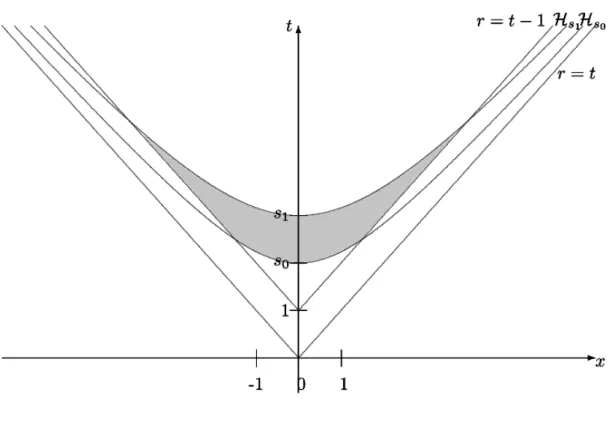
This set is thus limited by two hyperboloids and is naturally foliated by hyperboloids. See Fig. 2.1 for a display of the set K_rs0,s1s.

Taking now s1 “ `8, we will use the notation

K_rs0,_`8q :“ pt, xqL|x| † t ´ 1, ps0q2 § t2´ |x|2

(

“ §

s•s0

pHsX Kq. (2.1.4)

We refer to Fig. 2.2 for a display of this set.

In the following, we will be interested in functions supported in the conical region K_rs0,_`8q. Observe that the set K_rs0,_`8q is neither closed nor open and a function supported in this set, by definition, vanishes near the future light cone tr “ t ´ 1u but can be non-vanishing on the surface Hs0.

(24)

Fig. 2.1 The set K_rs₀_,s₁_s.

The region K X t|x| § t{2u will be also of interest in our estimates below, when we will investigate the behavior of solutions away from the light cone. Note in passing that the uniform estimate t § 2?₃3s holds in KX t|x| § t{2u.

We consider first the Klein-Gordon equation lu ` 2_u_{“ f,}

upt, xq|H_s0 “ u0pt, xq, utpt, xq|H_s0 “ u1pt, xq,

(2.1.5) with given , s0 “ B ` 1 ° 1. Recall that the symbol l denotes the

wave operator in Minkowski spacetime whose metric has the signature p1, ´1, ´1, ´1q. In (2.1.5), the initial data u0, u1 are prescribed and

com-pactly supported in the ball |x| § B( of radius B “ s0´ 1. The

source-term function f is supported in K_rs0,_`8q, so that, by the principle of prop-agation at finite speed, the solution u“ upt, xq to (2.1.5) is also supported in K_rs0,_`8q. In the same manner, the solution of the main system (1.2.1) studied in this monograph is also supported in K_rs0,_`8q and vanishes in a

neighborhood of the light cone r“ t ´ 1(.

Next, let us introduce the hyperbolic rotations or Lorentz boosts (by rising and lowering the indices with the Minkowski metric with

(25)

signa-Fig. 2.2 The set K_rs₀_,`8q.

ture p`, ´, ´, ´q)

La :“ ´xaB0 ` x0Ba “ xaBt ` tBa, (2.1.6)

which are tangent vectors to the hyperboloids. Denote by Z the family of admissible vector fields consisting of all vectors

Z↵ :“ B↵, Z3`a :“ La. (2.1.7)

Observe that, for any Z, Z1 P Z , the Lie bracket rZ, Z1s also belongs to Z , so that this set is a Lie algebra. For any multi-index I “ p↵1, ↵2, . . . , ↵mq

of length |I| :“ m, we denote by ZI the m-th order di↵erential operator ZI _:_{“ Z}

↵1. . . Z↵m. We also denote byBI the m-th order derivative operator

BI _:_{“ B}

↵1B↵2. . .B↵m (here 0 § ↵i § 3) and LI the m-th order derivative

operator LI _:_{“ L}

↵1L↵2. . . L↵m (here 4§ ↵j § 6).

Since we will be working within K, we have |xa{t| § 1 in K and, there-fore, the spatial rotations

⌦ab :“ xaBb´ xbBa (2.1.8)

need not be included explicitly in our analysis, since these fields can be recovered from Z via the identities

⌦ab “ x a

t Lb´ xb

(26)

Within the cone K, the coefficients xa_{{t are smooth, bounded, and}

homo-geneous of degree zero (see also Lemma 2.2.1).

Now we study the energy associated with the hyperboloidal foliation. Using Btu as multiplier for the equation (2.1.5), it is easy to derive the

following energy inequality for all s1 • s0:

` Em, ps1, uq ˘1_{2 § `Em, ps0, uq ˘1_{2 ` ªs1 s0 ˆ ª Hs f2dx ˙1{2 ds, (2.1.10) where the energy on the hyperboloids is defined as⇤

Em, ps1, uq :“ ª H_s1 ´ _ÿ3 a“1 ` pxa_{tqB tu` Bau ˘2 ` pps1{tqBtuq2` 2u2 ¯ dx (2.1.11) with dx “ dx1_dx2_dx3_{. H¨}_{ormander (1997)) established a Sobolev-type}

estimate adapted to this inequality (cf. Lemma 7.6.1 therein, or refer to (5.1.1) in Chapter 5, below) and arrived at the L8 estimate

sup H_s1 t3{2|u| § C ÿ |I|§2 Em, ps1, ZIuq1{2 § C ÿ |I|§2 Em, ps0, ZIuq1{2 ` C ÿ |I|§2 ªs1 s0 ˆ ª HspZ I_f_q2_dx ˙1{2 ds, (2.1.12)

where the summations are over all admissible vector fields in Z . Impor-tantly, this argument yields the (optimal) rate of decay t´3{2 enjoyed by solutions to the Klein-Gordon equation.

2.2 Semi-hyperboloidal frame

Our analysis in the present work is based on the semi-hyperboloidal frame —as we call it— defined by†

B0 :“ Bt, Ba :“ t´1La “

`

xa{t˘Bt ` Ba. (2.2.1)

⇤_{The subscript refers to the Minkowski metric.}

†_{In contrast, a standard method relies on the so-called null frame containing two null}

(27)

The transition matrices between the semi-hyperboloidal frame and the nat-ural frame B , that is, B_↵ “ _↵B and B↵ “ ↵B are found to be

:“ ¨ ˚ ˚ ˝ 1 0 0 0 x1{t 1 0 0 x2{t 0 1 0 x3{t 0 0 1 ˛ ‹ ‹ ‚, :“ ´1 “ ¨ ˚ ˚ ˝ 1 0 0 0 ´x1_{{t 1 0 0} ´x2_{{t 0 1 0} ´x3_{{t 0 0 1} ˛ ‹ ‹ ‚. (2.2.2)

With our choice of frame, the matrices , are smooth within the cone K. We adopt the following notation and convention. In order to express the components of a tensor in a frame, we always use Roman font with upper and lower indices for its components in the natural frame, while we use underlined Roman font for its components in the semi-hyperboloidal frame. Hence, a tensor is expressed as T “ T↵ _B

↵ b B in natural frame,

and as T “ T↵ B_↵b B in the semi-hyperboloidal frame. For example, the Minkowski metric is expressed in the semi-hyperboloidal frame as

m “ m↵ B_↵b B with ` m↵ ˘“ ¨ ˚ ˚ ˝ s2{t2 x1{t x2{t x3{t x1{t ´1 0 0 x2{t 0 ´1 0 x3_{{t 0} ₀ _´1 ˛ ‹ ‹ ‚ (2.2.3) and ` m_↵ ˘ “ ¨ ˚ ˚ ˝ 1 x1{t x2{t x3{t x1_{{t px}1_{tq2 _{´ 1 x}1_x2_{t2 _x1_x3_{t2 x2{t x2x1{t2 px2{tq2 ´ 1 x2x3{t2 x3{t x3x1{t2 x3x2{t2 px3{tq2 ´ 1 ˛ ‹ ‹ ‚. (2.2.4)

Similarly, a second-order di↵erential operator T↵ B↵B can be written

in the semi-hyperboloidal frame, so that by writing T↵ “ T↵1 1 1 ↵_↵1

(with obvious notation), we obtain the following decomposition formula for any function u

T↵ B↵B u “ T↵ B↵B u ` T↵ pB↵ 1

qB 1u. (2.2.5)

In particular, for the wave operator, we obtain lu “ m↵ _B ↵B u ` m↵ ` B↵ 1 ˘ B 1u, (2.2.6)

where we know that m00 “ pt2´ r2q{t2 “ s2{t2. This leads us immediately to the following key identity.

(28)

Proposition 2.2.1 (Semi-hyperboloidal decomposition of l). In the semi-hyperboloidal frame, the wave operator admits the decomposition

ps{tq2_B 0B0u “ lu ´ m0aB0Bau´ ma0BaB0u´ mabBaBbu ´ m↵ `_B ↵ 1 ˘ B 1u. (2.2.7) We will also need the following property.

Proposition 2.2.2. For any two-tensor T defined in the cone K and for all indices ↵, , I and admissible field Z, one has

ˇ ˇZI_T↵ ˇ_{ˇ À} ÿ ↵1 , 1 |I1|§|I| ˇ ˇZI1_T↵1 1ˇ_ˇ _{in K.}

The proof of this result (given below) will rely on the following two lemmas.

Lemma 2.2.1 (Homogeneity lemma). Let f “ fpt, xq be a smooth function defined in the closed region tt • 1, |x| § tu and assumed to be homogeneous of degree ⌘ in the sense that:

fppt, pxq “ p⌘fpt, xq for all p• 1{t. (2.2.8) For all multi-indices I1, I2, the following estimate holds for some positive

constant Cpn, |I1|, |I2|, fq: ˇ ˇBI1_ZI2_f_{pt, xq}ˇ_{ˇ § Cpn, |I} 1|, |I2|, fq t´|I1|`⌘ in K “ |x| † t ´ 1 ( . (2.2.9) Proof. We observe that Baf is homogeneous of degree ⌘ ´ 1 and Laf is

homogeneous of degree ⌘. We also observe that if some functions fi are

homogeneous of degree ⌘i, then the product±_ifi is homogeneous of degree

∞

i⌘i and then any ZIf is homogeneous.

We claim that the degree of homogeneity of ZIf , denoted by ⌘1, is not higher than ⌘. This can be checked by induction, as follows. Namely, this is clear when |I| “ 1. Moreover, assume that for all |I| § m, ZIf is homogeneous of degree ⌘1 § ⌘, then we now check the same property for all |I| “ m ` 1. Namely, assume that ZI _{“ Z}

1ZI 1

with |I1| “ m. When Z1 “ B↵, then ZIf “ B↵

`

ZI1f˘ and we observe that ZI1f is homogeneous of degree ⌘1 § ⌘. We see that B↵

`

ZI1_f˘ _{is again homogeneous of degree}

⌘1 ´ 1 † ⌘1 § ⌘. When Z1 “ La, then La

`

ZI1f˘ is homogeneous of degree ⌘1 § ⌘. This completes the induction argument that ZIf is homogeneous of degree ⌘ at most.

(29)

Furthermore, observe that if f is homogeneous of degree ⌘, then BI1f is homogeneous of degree ⌘ ´ |I1|. This is so since B↵f is homogeneous

of degree ⌘´ 1. Hence, BI1ZI2f is homogeneous of degree ⌘´ |I1| and is

smooth within the cone K.

Next, in order to establish (2.2.9), we take pt, xq P K and compute BI1_ZI2_f_{pt, xq “ t}_´|I1|`⌘1BI1_ZI2_fp1, x{tq _{with ⌘}1 § ⌘. _(2.2.10)

By a continuity argument in the compact set tt “ 1, |x| § 1u, there exists a positive constant Cpn, |I1|, |I2|q such that

sup

|x|§1

ˇ

ˇBI1_ZI2_f_{p1, xq}ˇ_{ˇ § Cpn, |I}

1|, |I2|q,

so that, in view of (2.2.10), the desired result is proven.

We now estimate the coefficients of the matrices and . First, we observe that xa{t is homogeneous of degree 0 and smooth in the closed region tt • 1, |x| § tu.

Lemma 2.2.2 (Changes of frame). With the notation above, the fol-lowing two estimates hold for all multi-indices I1, I2:

ˇ ˇBI1_ZI2 ↵ ˇ ˇ § Cpn, |I1|, |I2|q t´|I1| in K. (2.2.11) ˇ ˇBI1_ZI2 ↵ ˇ ˇ § Cpn, |I1|, |I2|q t´|I1| in K. (2.2.12)

Proof of Proposition 2.2.2. From T↵ “ T↵1 1 ↵_↵1 ↵1 we find

ZIT↵ “ ZI`T↵1 1 ↵_↵1 ↵1˘“ ÿ I1_`I2“I ZI1` ↵_↵1 ↵1˘ZI2T↵ 1 1 and, therefore, ˇ ˇZI_T↵ ˇ_{ˇ §} ÿ I1`I2“I ˇ ˇZI1` ↵ ↵1 ↵1˘ˇˇˇˇZI2T↵ 1 1ˇ ˇ §Cp|I|q ÿ |I2|§|I| ˇ ˇZI2_T↵1 1ˇ_ˇ.

Here, we have used that ˇˇZI1` ↵_↵1 ↵1˘ˇˇ § Cp|I1|q which follows from

(30)

2.3 Energy estimate for the hyperboloidal foliation

As presented in Chapter 1, we are interested in the following class of wave-Klein-Gordon type systems

lwi` Gj↵i B↵B wj ` c2iwi “ Fi,

wi|H_s0 “ wi0, Btwi|H_s0 “ wi1,

(2.3.1) with unknowns wi(1 § i § n0), where the metric Gj↵_i (with some abuse of

notation) and the source-terms Fi are supported in the cone K_rs0,_`8q, and

wi0, wi1 are supported on the initial hypersurface Hs0XK. To guarantee the

hyperbolicity, we assume the symmetry conditions (1.2.2). For definiteness, we may also assume (1.2.3) on the constants ci.

We introduce the following energy associated with the Minkowski metric on each hyperboloid Hs: Em,cips, wiq :“ ª Hs ˆ pBtwiq2` ÿ a pBawiq2` p2xa{tqBtwiBawi` c2iwi2 ˙ dx “ ª Hs ˆ ÿ a pBawiq2` ` ps{tqBtwi ˘2 ` c2 iw2i ˙ dx “ ª Hs ˆ ÿ a ` ps{tqBawi ˘2 ` t´2pSwiq2` t´2 ÿ a†b ` ⌦abwi ˘2 ` c2 iwi2 ˙ dx, (2.3.2) where we use the notation (2.1.8) and

t´1S :“ Bt`

ÿ

a

pxa_{tqB

a. _(2.3.3)

When ci “ 0, we may also write Emps, wiq :“ Em,0ps, wiq for short.

On the other hand, the curved energy which is naturally associated with the principal part of (2.3.1) is defined as

EG,cips, wiq :“ Em,cips, wiq ` 2 ª Hs ` BtwiB wjGj↵_i ˘ 0§↵§3¨ p1, ´x{tqdx ´ ª Hs ` B↵wiB wjGj↵i ˘ dx, (2.3.4) where the second term in the right-hand side involves the Euclidian inner product of the vectors `BtwiB wjGj↵i

˘

(31)

Proposition 2.3.1 (Hyperboloidal energy estimate). Given a con-stant 1 ° 1 and some locally integrable functions L, M • 0, the following

property holds. Let pwiq1_§i§n0 be the (local-in-time) solution to (2.3.1)

de-fined on some hyperbolic time interval rs0, s1s and suppose that the metric

and source satisfy the following coercivity conditions ´2₁ ÿ i Em,cips, wiq § ÿ i EG,cips, wiq § 21 ÿ i Em,cips, wiq, (2.3.5) ˇ ˇ ˇ ˇ ª Hs s t ˆ B↵Gj↵i BtwiB wj ´ 1 2BtG j↵ i B↵wiB wj ˙ dx ˇ ˇ ˇ ˇ § MpsqEm,cips, wiq1{2, (2.3.6)

and the bound

ÿ

i

}Fi}L2_pHsq § Lpsq, s P rs₀, s₁s. (2.3.7)

Recall also that the symmetry conditions (1.2.2) are assumed, that is, Gj↵_i “ Gi↵_j “ G_ij ↵, and that Fi, Gj↵i are supported in Krs0,s1s. The

following energy estimate holds (for all sP rs0, s1s):

ˆ ÿ i Em,cips, wiq ˙1{2 § 2 1 ˆ ÿ i Em,cips0, wiq ˙1{2 ` C2 1 ªs s0 ` Lp⌧q ` Mp⌧q˘d⌧, (2.3.8)

where the constant C ° 0 depends on the the structure of the system (2.3.1) only.

The following remarks are in order:

‚ In view of (2.3.2) and (2.3.8), the L2 _{norm of} _B

awi and ps{tqB↵wi

are uniformly controlled on each hypersurface Hs. It is expected

that these weighted expressions enjoy better decay thanB↵wi itself.

‚ In view of ∞apxa{rq

`

pr{tqBa ` pxa{rqBt

˘

wi “ t´1Swi, we see that

the weighted scaling derivative t´1Swi is also controlled.

‚ In Chapter 6, we will see that the energy Emps0, wiq on the initial

hyperboloid is controlled by the H1 norm of the initial data on the initial slice t “ s0.

(32)

Proof. In view of the symmetry (1.2.2) and by using Btwi as a multiplier,

we easily derive the energy identity ÿ i 1 2Bt ˆ ÿ ↵ pB↵wiq2` c2iw2i ˙ ´ÿ i ÿ a Ba ` BawiBtwi ˘ `ÿ i B↵ ` Gj↵_i BtwiB wj ˘ ´ÿ i 1 2Bt ` Gj↵_i B↵wiB wj ˘ “ ÿ i BtwiFi` ÿ i ˆ B↵Gj↵i BtwiB wj ´ 1 2BtG j↵ i B↵wiB wj ˙ .

We integrate this identity over the region K_rs0,s_s and use Stokes’ formula. Note that by the property of propagation at finite speed, the solutionpwiq

is defined in K_rs_0,_`8q and vanishing in a neighborhood of the light cone. By our assumption on the support of Gj↵_i , we obtain

1 2 ÿ i ` EG,cips, wiq ´ EG,cips0, wiq ˘ “ ÿ i ª K_rs0,ss ´ BtwiFi` B↵Gj↵_i BtwiB wj ´ 1 2BtG j↵ i B↵wiB wj ¯ dtdx “ ÿ i ªs s0 ˆ ª H⌧ p⌧{tqBtwiFidx ˙ d⌧ `ÿ i ªs s0 ˆ ª H⌧p⌧{tq ´ B↵Gj↵i BtwiB wj ´ 1 2BtG j↵ i B↵wiB wj ¯ dx ˙ d⌧, which leads us to d ds ÿ i EG,cips, wiq “2 ÿ i ª Hs ´ ps{tqB↵Gj↵_i BtwiB wj ´ ps{2tqBtGj↵_i B↵wiB wj ` ps{tqBtwiFi ¯ dx. So, with the assumptions (2.3.6) and (2.3.7), we get

ˆ ÿ i EG,cips, wiq ˙1{2 d ds ˆ ÿ i EG,cips, wiq ˙1{2 § ÿ i ˆ Mpsq ` }Fi}L2_pH_s_q ˙ Em,cips, wiq1{2 § CMpsq´ ÿ i Em,cips, wiq ¯1{2 ` C´ ÿ i }Fi}2L2_pH sq ¯1{2´ ÿ i Em,cips, wiq ¯1{2 “ C´Mpsq ` Lpsq¯´ ÿ i Em,cips, wiq ¯1{2 § C1 ` Mpsq ` Lpsq¯ ´ ÿ i EG,cips, wiq ¯1{2 ,

(33)

which yields d ds ˆ ÿ i EG,cips, wiq ˙1{2 § C1 ` Lpsq ` Mpsq˘. We integrate this inequality over the interval rs0, ss and obtain

ˆ_ÿn0 i“1 EG,cips, wiq ˙1_{2 § ˆ_ÿn0 i“1 EG,cips0, wiq ˙1_{2 ` C1 ªs s0 Lp⌧qd⌧ ` C1 ªs s0 Mp⌧qd⌧. By using the condition (2.3.5), this completes the proof.

2.4 The bootstrap strategy

We are now in a position to outline our method of proof of Theorem 1.2.1. From now on, we assume that the assumptions therein are satisfied. It will be necessary to distinguish between three levels of regularity and, in order to describe this scale of regularity, we will use the following convention on the indices in use:

I7: multi-index of order § 5, I:: multi-index of order § 4, I: multi-index of order § 3,

(2.4.1) which we call admissible indices. Throughout, C, C0, C1, C⇤, . . . are

constants depending only on the structure of the system (1.2.1), such as j0, k0, B, ci.

We will use certain norms on the hyperboloids and, so, if u is a function supported in K_rs0,_`8q, we set (for s • s0):

}u}Lp_pHsq :“ ˆ ª Hs ˇ ˇupt, xqˇˇp dx ˙1{p “ ˆ ª R3 ˇ ˇu`as2_{` |x|}2_{, x}˘ˇˇp_dx ˙1{p . (2.4.2) The proof of Theorem 1.2.1 relies on Propositions 2.4.1–2.4.3, stated now. The first proposition below concerns the construction of initial data on the initial hyperboloid HB`1, and will be established in Chapter 11.

Proposition 2.4.1 (Initialization of the argument). For any suffi-ciently large constant C0 ° 0, there exists a positive constant ✏10 P p0, 1q

depending only on B and C_ÿ 0 such that, for every initial data satisfying i

`

(34)

the local-in-time solution to (1.2.1) associated with this initial data extends to the region limited by the constant time hypersurface t “ B ` 1 and the hyperboloid HB_`1. Furthermore, it satisfies the uniform bound

ÿ

j

Emps0, ZI 7

wjq1{2 § C0✏. (2.4.4)

for all admissible vector fields Z and all admissible indices I7.

Given some constants C1, ✏ ° 0 and P p0, 1{6q and a hyperbolic time

interval rs0, s1s, we call hierarchy of energy bounds with parameters

pC1, ✏, q the following five inequalities (for all s P rs0, s1s and all admissible

fields and admissible indices): Emps, ZI 7 u_pıq1{2 § C1✏s for 1§ pı § j0, (2.4.5a) Em, ps, ZI 7 v_q|q1{2 § C1✏s for j0` 1 § q|§ n0, (2.4.5b) Emps, ZI : u_pıq1{2 § C1✏s {2 for 1 § pı § j0, (2.4.5c) Em, ps, ZI : v|_qq1{2 § C1✏s {2 for j0` 1 § q|§ n0, (2.4.5d) Emps, ZIupıq1{2 § C1✏ for 1§ pı § j0. (2.4.5e)

Observe that (2.4.5e) concerns the wave components only and that the upper bound is independent of time.

At this juncture, since c_qı• ° 0 for all j0` 1 § qı § n0, we have

Em, ps, ZI 7 v_qıq § Em,c_qıps, ZI 7 v_qıq § pc_qı{ q2Em, ps, ZI 7 v_qıq, (2.4.6) so that the two energy expressions are equivalent.

Given some constants 1 ° 1, C⇤, C1, ✏° 0 and P p0, 1{6q and a

hyper-bolic time interval rs0, s1s, we call hierarchy of metric-source bounds

with parameters p1, C⇤, C1, ✏, q. the following three sets of estimates:

‚ For all |I7| § 5, ´2₁ ÿ i EG,cips, ZI 7 wiq § ÿ i Em,cips, ZI 7 wiq § 21 ÿ i EG,cips, ZI 7 wiq, (2.4.7a) ˇ ˇ ˇ ˇ ª Hs s t ˆ B↵Gj↵i BtZI 7 wiB ZI 7 wj ´ 1 2BtG j↵ i B↵ZI 7 wiB ZI 7 wj ˙ dx ˇ ˇ ˇ ˇ § C⇤_pC 1✏q2s´1` Em,cips, ZI 7 wiq1{2 “: MpI7, sqEm,cips, ZI 7 wiq1{2, (2.4.7b)

(35)

and⇤ n0 ÿ i_“1 › ›rGj↵ i B↵B , ZI 7 swj › › L2_pHsq` n0 ÿ i_“1 › ›ZI7_F i › › L2_pHsq § C⇤_pC 1✏q2s´1` “: LpI7, sq. (2.4.7c) ‚ For all |I_ˇ :| § 4, ˇ ˇ ˇ ª Hs s t ˆ B↵Gj↵_i BtZI : wiB ZI : w_p|´ 1 2BtG j↵ i B↵ZI : wiB ZI : wj ˙ dx ˇ ˇ ˇ ˇ § C⇤_pC 1✏q2s´1` {2Em,cips, ZI : wiq1{2 “: MpI:, sqEm,cips, ZI : wiq1{2 (2.4.8a) and n0 ÿ i“1 › ›rGj↵ i B↵B , ZI : swj › › L2_pHsq` n0 ÿ i“1 › ›ZI:_F i › › L2_pHsq § C⇤_pC 1✏q2s´1` {2 “: LpI:, sq. (2.4.8b) ‚ For all |I| § 3,

ˇ ˇ ˇ ˇ ª Hs s t ˆ B↵Gj↵_pı BtZIupıB ZIu|p´ 1 2BtG j↵ pı B↵ZIupıB ZIup| ˙ dx ˇ ˇ ˇ ˇ § C⇤_pC 1✏q2s´3{2`2 Emps, ZIupıq1{2 “: MpI, sqEmps, ZIupıq1{2 (2.4.9a) and n0 ÿ i_“1 › ›rGj↵ i B↵B , ZIswj › › L2_pHsq ` n0 ÿ i“1 › ›ZI_F i › › L2_pH_s_q` }Z I`_Gq|↵ pı B↵B vq| ˘ }L2_pH sq § C⇤_pC 1✏q2s´3{2`2 “: LpI, sq. (2.4.9b)

Observe that (2.4.9a) concerns the wave components, only.

Proposition 2.4.2. Fix some P p0, 1{6q. There exists a positive constant ✏2₀ such that for all ✏, C1 ° 0 with C1✏ § 1 and C1✏ § ✏20, there exists a

constant 1 ° 1 and a constant C⇤ ° 0 (both determined by the structure

of the system (1.2.1)) such that the hierarchy of energy bounds (2.4.5) with parameters C1, ✏, implies the hierarchy of metric–source bounds (2.4.7a)—

(2.4.9b) with parameters 1, C⇤, C1, ✏, .

(36)

The proof of this proposition will occupy a major part of this mono-graph, especially Chapters 7 to 10. Now we admit this proposition and give the proof of the main result, which is going to be essentially based on the following observation.

Proposition 2.4.3 (Enhancing the hierarchy of energy bounds). Let P p0, 1{6q and let C0 ° 0 be a constant and C1 ° C0 be a sufficiently

large constant. Then, there exists ✏1 ° 0 such that the following

enhanc-ing property holds. For any solution pwiq to (1.2.1) defined in K_rs0,s1s and

provided, for ✏P r0, ✏1s,

(1) ∞n0_i_“1Em,cips0, ZI 7

wiq1{2 § C0✏ for all admissible Z and I7,

(2) the hierarchy (2.4.5) holds with parameters pC1, ✏, q in the time

interval rs0, s1s,

then the following improved energy estimates also hold Emps, ZI 7 u_pıq1{2 § 1 2C1✏s for 1 § pı § j0, (2.4.10a) Em, ps, ZI 7 v_q|q1{2 § 1 2C1✏s for j0 ` 1 § q|§ n0, (2.4.10b) Emps, ZI : u_pıq1{2 § 1 2C1✏s {2 _{for 1} _{§ pı § j} 0, (2.4.10c) Em, ps, ZI : v_q|q1{2 § 1 2C1✏s {2 _{for j} 0` 1 § q|§ n0, (2.4.10d) Emps, ZIupıq1{2 § 1₂C1✏ for 1§ pı § j0. (2.4.10e)

Proof. We will use here the conclusion of Proposition 2.4.2. We assume that ✏1 is sufficiently small with ✏1 § C₁´1mint1, ✏20u such that, for all

✏§ ✏1, the conclusion in Proposition 2.4.2 holds.

Step I. High-order energy estimates. To the equations (1.2.1), we apply the operator ZI7 (with |I7| § 5 throughout) and obtain

lpZI7_w iq ` Gj↵_i B↵B pZI 7 wjq ` c2iZI 7 wi “ rGj↵_i B↵B , ZI 7 swj ` ZI 7 Fi.

In view of Proposition 2.3.1 and thanks to the conditions (2.4.7a)–(2.4.7c) implied by Proposition 2.4.2, we find

ˆ ÿ i Em,cips, ZI 7 wiq ˙1_{2 § 2 1 ˆ ÿ i Em,cips0, ZI 7 wiq ˙1{2 ` C2 1 ªs s0 ` LpI7, ⌧q ` MpI7, ⌧q˘d⌧.

(37)

In view of Proposition 2.4.2 combined with the condition (1) in the propo-sition, we then have

ˆ ÿ i Em,cips, ZI 7 wiq ˙1{2 § 2 1C0✏` C21C⇤pC1✏q2 ªs s0 ⌧´1` d⌧. Choosing ✏1 § pC1´2 2 1C0q 2CC⇤_2 1C12 , we obtain ˆ ÿ i Em,cips, ZI 7 wiq ˙1{2 § 1 2C1✏s , which leads to the enhanced energy bound

Em, ps, ZI 7 wiq1{2 § Em,cips, ZI 7 wiq1{2 § 1 2C1✏s . (2.4.11) This establishes (2.4.10b)-(2.4.10a).

Step II. Intermediate energy estimates. We will next rely on the metric–source bounds (2.4.8a)-(2.4.8b) (with |I:| § 4 throughout) given by the conclusion of Proposition 2.4.2. To the equation (1.2.1), we apply the operator ZI: and obtain

lpZI:_w iq ` Gj↵_i B↵B pZI : wjq ` c2iZI : wi “ rGj↵_i B↵B , ZI : swj ` ZI : Fi.

From Proposition 2.3.1 and thanks to the conditions (2.4.7a) and (2.4.8a)-(2.4.8b), we find ˆ ÿ i Em,cips, ZI : wiq ˙1{2 § 2 1 ˆ ÿ i Em,cips0, ZI : wiq ˙1_{2 ` C2 1 ªs s0 ` LpI:, ⌧q ` MpI:, ⌧q˘d⌧. We thus have ˆ ÿ i Em,cips, ZI : wiq ˙1{2 § 2 1C0✏` C21C⇤pC1✏q2 ªs s0 ⌧´1` {2d⌧. Provided ✏ is sufficiently small so that ✏1 § pC1´2

2 1C0q 4CC⇤_2 1C21 , we find ˆ ÿ i Em,cips, ZI : wiq ˙1{2 § 1₂C1✏s {2,

which leads to the enhanced energy bound Em, ps, ZI : wiq1{2 § Em,cips, ZI : wiq1{2 § 1 2C1✏s {2. (2.4.12)

(38)

This establishes (2.4.10d)-(2.4.10c).

Step III. Low-order energy estimates. We will now rely on the metric– source bounds (2.4.9a)-(2.4.9b) (with|I| § 3 throughout). We apply ZI _to

In view of Proposition 2.3.1 and thanks to the conditions (2.4.7a) and (2.4.9a)-(2.4.9b), we obtain ˆ ÿ pı Emps, ZIupıq ˙1{2 § 2 1 ˆ ÿ pı Emps0, ZIupıq ˙1_{2 ` C2 1 ªs s0 ` LpI, ⌧q ` MpI, ⌧q˘d⌧ and, therefore, ˆ ÿ pı Emps, ZIupıq ˙1{2 § 2 1C0✏` C21C⇤pC1✏q2 ªs s0 ⌧´3{2`2 d⌧. By recalling that † 1{6, it follows that

ˆ ÿ pı Emps, ZIupıq ˙1{2 § 2 1C0✏` CC⇤2₁C₁2✏2pB ` 1q2 ´1{2 p1{2q ´ 2 . Provided ✏1 § p1´4 qpC1´2 2 1C0q 4CC⇤_2

1C1pB`1q2 2 ´1{2, we obtain the enhanced energy bound

for the wave components

Emps, ZIupıq1{2 §

1 2C1✏ and this establishes (2.4.10e).

Step IV. In conclusion, by assuming that ✏1 § min´ pC1´ 2 2 1C0q 4CC⇤_2 1C12 , p1 ´ 4 qpC1´ 2 2 1C0q 4CC⇤_2 1C12pB ` 1q2 ´1{2 , ✏2₀, C₁´1¯, all conditions (2.4.10) are satisfied and the proof is completed.

Observe that (2.4.7a), (2.4.7b), (2.4.8a), and (2.4.9a) concern only the “metric” Gj↵_i and depend mainly on L8 bounds on the solution and its derivatives: these bounds will be established in Chapter 9. On the other hand, the inequalities (2.4.7c), (2.4.8b), and (2.4.9b) are L2 _{type estimates}

and will be derived later in Chapter 10.

We complete this chapter with a proof of our main result —by assuming that Propositions 2.4.1 and 2.4.2 are established.

(39)

Proof of Theorem 1.2.1. Let pwiq be the unique local-in-time solution

to (1.2.1) associated with the initial data pwi0, wi1q. Given our assumption

on the support of pwi0, wi1q and according to the property of propagation

at finite speed, this solutionpwiq must be supported in the region K_rs0,_`8q.

As guaranteed by Proposition 2.4.1, there exist constants C0, ✏10 such

that, provided }w_i0}_H6_pR3_q ` }w_i1}_H5_pR3_q § ✏ § ✏1₀, we have the energy

bound EGps0, ZI 7

wjq1{2 § C0✏.

Let rs0, s⇤s be the largest time interval (containing s0) on which (2.4.5)

holds with some parameters C1, ✏ ° 0 and P p0, 1{6q fixed and for a

sufficiently large constant C1 ° C0. By continuity, we have s⇤ ° s0.

Proceeding by contradiction, let us assume that s⇤ † `8, so that at the time s “ s⇤, one (at least) of the inequalities (2.4.5) must be an equality. That is, at least one of the following conditions holds:

Em, ps⇤, ZI 7 v_q|q1{2 “ C1✏s⇤ for j0` 1 § q|§ n0, Emps⇤, ZI 7 u_pıq1{2 “ C1✏s⇤ for 1§ pı § j0, Em, ps⇤, ZI : v|_qq1{2 “ C1✏s⇤ {2 for j0 ` 1 § q|§ n0, Emps⇤, ZI : u_pıq1{2 “ C1✏s⇤ {2 for 1§ pı § j0, Emps⇤, ZIupıq1{2 “ C1✏, for 1§ pı § j0. (2.4.13)

Yet, according to Proposition 2.4.3 there exists ✏1 ° 0 such that, for ✏ § ✏1,

the following enhanced energy bounds also hold: Em, ps⇤, ZI 7 v|_qq1{2 § 1 2C1✏s ⇤ _{for j} 0` 1 § q|§ n0, Emps⇤, ZI 7 u_pıq1{2 § 1 2C1✏s ⇤ _{for 1}_{§ pı § j} 0, Em, ps⇤, ZI : v_q|q1{2 § 1 2C1✏s ⇤ {2 _{for j} 0` 1 § q|§ n0, Emps⇤, ZI : u_pıq1{2 § 1 2C1✏s ⇤ {2 _{for 1}_{§ pı § j} 0, Emps⇤, ZIupıq1{2 § 1 2C1✏ for 1§ pı § j0. Clearly, this is impossible, unless s⇤ “ `8.

Hence, we have proven that the inequalities (2.4.5) hold for all s P rs0,`8q and, by the local existence criteria in Theorem 11.2.1 (combined

with Sobolev’s inequality), this local solution extends for all times. By taking ✏0 :“ min

` ✏1₀, ✏1

˘

(40)

2.5 Energy on the hypersurfaces of constant time

To end this chapter, we prove that the wave components of the global-in-time solutions which we have constructed for (1.2.1) enjoy a uniform energy estimate also on the standard hypersurfaces of constant time t.

Proposition 2.5.1. Consider the wave components ui of a global-in-time

solution wi satisfying (2.4.5) and (2.4.9) (with ✏0 sufficiently small and

C1✏ † 1). The following estimate also holds for all time t • B ` 1:

}BtZIupt, ¨q}L2_pR3_q` ÿ a }BaZIupt, ¨q}L2_pR3_q § C3pB, , ✏0qC1✏, (2.5.1) where C3 depends upon , ✏0 and the structure of the system only.

The proof of this result relies on a modified version of the fundamental energy estimate, as now stated.

Lemma 2.5.1. Let puiq be the solution to the Cauchy problem

lui` Gj↵i B↵ ui“ Fi,

ui|H_s0 “ ui0, Btui|H_s0 “ ui0,

(2.5.2) where Fi and Gj↵_i are defined in K_rs0,_`8q, while ui|H_s0,Btui|H_s0 are

sup-ported in Hs0 X K. There exists "0 ° 0 such that, provided

max

i,j,↵, |G j↵

i | § "0,

there exists a positive constant C “ Cp✏0q such that

ˆ }Btupt0,¨q}L2_pR3_q` ÿ a }Baupt0,¨q}L2_pR3_q ˙2 § Cÿ i EGpt, uiq ` C ÿ i ª_pt2_0`1q{2 t0 ª Hs ps{tqˇˇBtuiFi ˇ ˇ dxds ` C ª_pt2_0`1q{2 t0 ª Hs ps{tqˇˇB↵Gj↵_i BtuiB uj ´ 1 2BtG j↵ i B↵uiB uj ˇ ˇ dxds. (2.5.3) Proof. The proof relies on an energy estimate within the region Kt0 :“

tpt, xqˇˇ|x| § t ´ 1, t0 § t §

a

|x|2_{` t}2

(41)

Fig. 2.3 The region Kt0

begin from the general identity ÿ i ˆ 1 2Bt ÿ ↵ ` B↵ui ˘2 `ÿ a Ba ` BauiBtui ˘ ` B↵ ` Gj↵_i BtuiB uj ˘ ´ 1 2Bt ` Gj↵_i B↵uiB uj ˘˙ “ÿ i BtuiFi` ÿ i ˆ B↵Gj↵i BtuiB uj ´ 1 2BtG j↵ i B↵uiB uj ˙

and we integrate it within Kt0 with respect to the volume form dtdx.

Applying Stokes’ formula, we find 1 2 ÿ i EGpt, uiq ´ 1₂ÿ i ª R3 ˆ ÿ ↵ |B↵ui|2` 2Gj0_i BtuiB uj ´ Gj↵_i B↵uiB uj ˙ pt, ¨qdx “ ª K_t0 ÿ i ˆ BtuiFi` B↵Gj↵_i BtuiB uj ´ 1 2BtG j↵ i B↵uiB uj ˙ dxdt “ ª K_t0ps{tq ÿ i ˆ BtuiFi` B↵Gj↵i BtuiB uj ´ 1 2BtG j↵ i B↵uiB uj ˙ dxds,

(42)

where we recall that s“ at2_{´ |x|}2_{. This implies} ÿ i ª R3 ˆ ÿ ↵ |B↵ui|2` 2Gj0_i BtuiB uj ´ Gj↵_i B↵uiB uj ˙ pt, ¨qdx §ÿ i EGpt, uiq `ÿ i ª K_t0ps{tq ˇ ˇBtuiFi` B↵Gj↵i BtuiB uj ´ 1 2BtG j↵ i B↵uiB uj ˇ ˇ dxds, which is bounded by ÿ i EGpt, uiq ` ÿ i ª_pt2_0`1q{2 t0 ª Hs ps{tqˇˇBtuiFi ˇ ˇ dxds ` ª_pt2_0`1q{2 t0 ª Hs ps{tqˇˇB↵Gj↵_i BtuiB uj ´ 1 2BtG j↵ i B↵uiB uj ˇ ˇ dxds. We then observe that

ÿ i ª R3 ˇ ˇ2Gj0 i BtuiB uj ´ Gj↵i B↵uiB uj ˇ ˇ dx § C max i,j,↵, |G j↵ i | ÿ i,↵ }B↵uipt, ¨q}L2_pR3_q

and thus, provided maxi,j,↵, |Gj↵i | is sufficiently small,

ÿ i ª R3 ˇ ˇ2Gj0 i BtuiB uj ´ G j↵ i B↵uiB uj ˇ ˇ dx § 1₂ÿ i,↵ }B↵uipt, ¨q}L2_pR3_q. We thus have 1 2 ÿ i,↵ }B↵upt, ¨q}L2_pR3_q § ÿ i ª R3 ˆ ÿ ↵ |B↵ui|2` 2Gj0i BtuiB uj ´ Gj↵i B↵uiB uj ˙ dx and the desired result is proven.

(43)

and apply (2.5.3), so that ÿ pı,↵ }B↵ZIupıpt, ¨q}L2_pR3_q § Cÿ pı EGpt, ZIupıq ` C ÿ pı ª_pt2_0`1q{2 t0 ª Hs ps{tqˇˇBtZIupıZIFpı ˇ ˇ dxds `ÿ pı ª_pt2_0`1q{2 t0 ª Hs ps{tqˇBˇ tZIupırG_pıp|↵ B↵B , ZIsup| ˇ ˇ dxds `ÿ pı ª_pt2_0`1q{2 t0 ª Hsps{tq ˇ ˇBtZIupıZI`G_pıq|↵ B↵B v|q˘ˇˇdxds ` Cÿ pı ª_pt2_0`1q{2 t0 ª Hs ps{tqˇˇB↵Gj↵_pı BtZIupıB ZIuj ´ 1 2BtG j↵ pı B↵ZIupıB ZIuj ˇ ˇdxds. By (2.4.5e) (which was established within our bootstrap argument and holds on the time interval rB ` 1, `8q), we have

ÿ

pı

EGpt, ZIupıq § pC1✏q2.

Also, the second term in the right-hand side is uniformly bounded, as fol-lows: ª_pt2_0`1q{2 t0 ª Hs ps{tqˇˇBtZIupıZIFpı ˇ ˇ dxds § ª_pt2_0`1q{2 t0 }ps{tqB tZIupı}L2_pH_s_q}ZIF_pı}_L2_pH_s_qds § C1✏ ª_pt2_0`1q{2 t0 }Z I_F pı}L2_pHsqds § C1✏ ª_pt2_0`1q{2 t0 CC⇤pC1✏q2s´3{2`2 ds § CC⇤_pC 1✏q3p1{2 ´ 2 q´1pB ` 1q´1{2`2 .

The third and fourth terms are bounded in the same manner, that is, ª_pt2_0`1q{2 t0 ª Hsps{tq ˇ ˇBtZIupırG_pı|↵p B↵B , ZIsu|p ˇ ˇ dxds § CC⇤_pC 1✏q3p1{2 ´ 2 q´1pB ` 1q´1{2`2 and ª_pt2_0`1q{2 t0 ª Hs ps{tqˇˇBtZIupıZI ` G_pı|↵q B↵B v|q˘ˇˇdxds § CC⇤_pC 1✏q3p1{2 ´ 2 q´1pB ` 1q´1{2`2 .

(44)

The last term is bounded by applying (2.4.9a): ª_pt2_0`1q{2 t0 ª Hs ps{tqˇˇB↵Gj↵_pı BtZIupıB ZIuj ´ 1 2BtG j↵ pı B↵ZIupıB ZIuj ˇ ˇ dxds § CC⇤_pC 1✏q3p1{2 ´ 2 q´1pB ` 1q´1{2`2 .

(45)

Chapter 3

Decompositions and estimates for the

commutators

3.1 Decompositions of commutators. I

In this chapter, we present technical results concerning the commutators rX, Y su :“ XpY uq ´ Y pXuq of certain operators X, Y associated with the set of admissible vector fields Z (cf. Chapter 2) and applied to functions u defined in the cone K “ t|x| † t ´ 1u. In order to derive uniform bounds, we will rely on homogeneity arguments and on the observation that all the coefficients in the following decomposition are smooth within K.

First of all, all admissible vector fields B↵, La under consideration are

Killing fields for the flat wave operatorl, so that the following commutation relations hold:

rB↵, ls “ 0, rLa, ls “ 0. (3.1.1)

By introducing the notation

rLa,B su “: ⇥_a B u, (3.1.2a)

rB↵,B su “: t´1 _↵ B u, (3.1.2b)

rLa,B su “: ⇥_a B u, (3.1.2c)

we find easily that

⇥_ab “ ´ _{ab 0}, ⇥_a0 “ ´ _a, ab “ ab 0, 0b “ ´ xb t 0 “ 0 b 0, ↵0 “ 0, ⇥_ab “ ´x b t a “ 0 b a, ⇥a0 “ ´ a ` xa t 0 “ ´ a ` a 0 0, (3.1.3) 35

(46)

where and were defined in (2.2.2). All of these coefficients are smooth in the cone K and for each index I, the functions ZI⇧ are bounded for all ⇧P ⇥, ⇥, (. Furthermore, we can also check that

⇥0_ab “ 0 so that rLa,Bbs “ ⇥abB “ ⇥cabBc. (3.1.4)

Lemma 3.1.1 (Algebraic decompositions of commutators. I). There exist constants ✓I_↵J such that, for all sufficiently regular function u defined in the cone K, the following identities hold for all ↵ and I:

rZI_,_B ↵su “

ÿ

|J|†|I|

✓_↵JI B ZJu. (3.1.5)

Proof. The proof is done by induction on |I|. When |I| “ 1, (3.1.5) is implied by (3.1.2a). Assume next that (3.1.5) is valid for |I| § k and let us derive this property for all |I| “ k ` 1. Let ZI be a product with index satisfying|I| “ k ` 1, where ZI _{“ Z}

1ZI 1

with |I1| “ k and Z1 is one of the

fields B , La. In view of rZI_,_B ↵su “ rZ1ZI 1 ,B↵su “ Z1 ` rZI1_,_B ↵su ˘ ` rZ1,B↵sZI 1 u and Z1 ` rZI1_,_B ↵su ˘ “ Z1 ˆ ÿ |J|§k´1 ✓_↵JI1 B ZJu ˙ “ ÿ |J|§k´1 ✓_↵JI1 Z1B ZJu, we have rZI_,_B ↵su “ ÿ |J|§k´1 ✓I_↵J1 Z1B ZJu` rZ1,B↵sZI 1 u.

First of all, if Z1 “ B , we have the commutation property

rZ1,B↵sZI 1 u “ 0 and ÿ |J|§k´1 ✓_↵JI1 Z1B ZJu “ ÿ |J|§k´1 ✓_↵JI1 B Z1ZJu,

so that (3.1.5) is established in this case.

Second, if Z1 “ La, we apply (3.1.2a) and write

ÿ |J|§k´1 ✓I1_↵J LaB ZJu “ ÿ |J|§k´1 ✓I_↵J1 B LaZJu` ÿ |J|§k´1 ✓_↵JI1 rLa,B sZJu “ ÿ |J|§k´1 ✓I_↵J1 B LaZJu` ÿ |J|§k´1 ✓_↵JI1 ⇥_a B ZJu. So, (3.1.5) holds for |I| “ k ` 1, which completes the induction argument.

(47)

3.2 Decompositions of commutators. II and III

Lemma 3.2.1 (Algebraic decompositions of commutators. II). For all sufficiently regular functions u defined in the cone K, the follow-ing identity holds:

rZI_,_{B su “} ÿ |J|†|I|

✓I_JB ZJu, (3.2.1)

where the functions ✓I_J are smooth and satisfy in K : ˇ ˇBI1_ZI2_✓I J ˇ ˇ § C`n,|I|, |I1|, |I2| ˘ t´|I1|. (3.2.2)

Proof. Consider the identity

rZI_,_{B su “ rZ}I_, _{B su “} ÿ I1`I2“I

|I2|†|I|

ZI1 ZI2B u ` rZI,B su. In the first sum, we commute ZI2 and B and obtain

rZI_,_{B su “} ÿ I1Ì2“I |I2|†|I| ZI1 B ZI2u` ÿ I1Ì2“I |I2|†|I| ZI1 rZI2,B su ` rZI,B su “ ÿ I1Ì2“I |I2|†|I| ZI1 B ZI2u` ÿ I1_Ì2“I ZI1 rZI2,B su “ ÿ I1Ì2“I |I2|†|I| ZI1 B ZI2u` ÿ I1Ì2“I |J|†|I2| ` ZI1 ˘✓I2↵_J B↵ZJu.

Hence, ✓I↵_J are linear combinations of ZI1 and ✓I2↵_J ZI1 with |I1| § |I|

and |I2| § |I|, which yields (3.2.1). Note that ✓I2↵_J are constants, so that

BI3_ZI4`_✓I2↵ J ZI1 ˘ “ ✓I2↵ J BI3ZI4ZI1 and, by (2.2.11), we arrive at (3.2.2).

Lemma 3.2.2 (Algebraic decompositions of commutators. III). For all sufficiently regular functions u defined in the cone K, the follow-ing identities hold:

rZI_,_B csu “ ÿ |J|†|I| Ib cJBbZJu` t´1 ÿ |J1_|†|I| ⇢I_cJ1B ZJ 1 u, (3.2.3)

where the functions I_cJ and ⇢I_cJ are smooth and satisfy in K: ˇ

ˇBI1_ZI2 I J

ˇ

ˇ § Cpn, |I|, |I1|, |I2|qt´|I1|, (3.2.4a)

ˇ

ˇBI1_ZI2_⇢I J

ˇ

(48)

Proof. We proceed by induction. The case |I| “ 1 is easily checked from (3.1.2b), (3.1.2c) and (3.1.4). Assuming that (3.2.3) with (3.2.4a) and (3.2.4b) hold for |I| § k, we consider indices |I| “ k ` 1. To do this, let ZI be a product of operators with index |I| “ k ` 1. Then, ZI “ Z1ZI

1

with |I1| “ k and the following holds: rZI_,_B csu “ rZ1ZI 1 ,B_cs “ Z1 ` rZI1_,_B csu ˘ ` rZ1,BcsZI 1 u. Case Z1 “ B↵. In this case, we write

Z1 ` rZI1_,_B csu ˘ “ B↵ ˆ ÿ |J|†|I1_| I1b cJBbZJu` t´1 ÿ |J1_|†|I1_| ⇢I_cJ11B ZJ 1 u ˙ “ ÿ |J|†|I1_| B↵ ` _I1_b cJ ˘ BbZJu` ÿ |J|†|I1_| I1b cJ BbB↵ZJu` ÿ |J|†|I1_| I1b cJ rB↵,BbsZJu ` B↵t´1 ÿ |J1_|†|I1_| ` ⇢I_cJ11˘B ZJ 1 u` t´1 ÿ |J1_|†|I1_| B↵ ` ⇢I_cJ11˘B ZJ 1 u ` t´1 ÿ |J1_|†|I1_| ⇢I_cJ11B B↵ZJ 1 u.

For the third term, we recall (3.1.2b) and write

I1b cJ rB↵,BbsZJu“ t´1 I 1_b cJ ↵bB ZJu. Hence, we find Z1 ` rZI1_,_B csu ˘ “ ÿ |J|†|I1_| B↵ ` _I1_b cJ ˘ BbZJu` ÿ |J|†|I1_| I1b cJ BbB↵ZJu` t´1 ÿ |J|†|I1_| I1b cJ ↵bB ZIu ` B↵t´1 ÿ |J1_|†|I1_| ` ⇢I_cJ11 ˘ B ZJ1_u_{` t}´1 ÿ |J1_|†|I1_| B↵ ` ⇢I_cJ11 ˘ B ZJ1_u ` t´1 ÿ |J1_|†|I1_| ⇢I_cJ11B B↵ZJ 1 u.

We conclude that, when Z1 “ B↵, I↵J are linear combinations of B↵ I 1_b cJ

and I_cJ1b with |J| † |I1|. For all BI1ZI2, we have BI1_ZI2`_B ↵ I 1_b cJ ˘ “B↵BI1ZI2 I 1_b cJ ` BI1 ` rZI2_,_B ↵s I 1_b cJ ˘ “B↵BI1ZI2 I 1_b cJ ` ÿ |I_2|†|I2|1 ✓I2_↵I1 2B B I1_ZI₂1 I2 cJ .