On the Onset of Stochasticity in $\Lambda$CDM Cosmological Simulations

HAL Id: hal-00266048

https://hal.archives-ouvertes.fr/hal-00266048

Preprint submitted on 20 Mar 2008

HAL is a multi-disciplinary open access

archive for the deposit and dissemination of

sci-entific research documents, whether they are

pub-lished or not. The documents may come from

teaching and research institutions in France or

abroad, or from public or private research centers.

L’archive ouverte pluridisciplinaire HAL, est

destinée au dépôt et à la diffusion de documents

scientifiques de niveau recherche, publiés ou non,

émanant des établissements d’enseignement et de

recherche français ou étrangers, des laboratoires

publics ou privés.

On the Onset of Stochasticity in ΛCDM Cosmological

Simulations

Jerome Thiebaut, Christophe Pichon, Thierry Sousbie, Simon Prunet, D.

Pogosyan

To cite this version:

Jerome Thiebaut, Christophe Pichon, Thierry Sousbie, Simon Prunet, D. Pogosyan. On the Onset of

Stochasticity in ΛCDM Cosmological Simulations. 2008. �hal-00266048�

hal-00266048, version 1 - 20 Mar 2008

On the Onset of Stochasticity in

_{ΛCDM Cosmological Simulations}

J. Thiebaut

, C. Pichon

, T. Sousbie

, S. Prunet

& D. Pogosyan

1

Institut d’astrophysique de Paris & UPMC (UMR 7095), 98, bis boulevard Arago , 75 014, Paris, France. 2

Service d’Astrophysique, IRFU,(UMR) CEA-CNRS, L’orme des meurisiers, 91 470, Gif sur Yvette, France. 3

Department of Physics, University of Alberta, 11322-89 Avenue, Edmonton, Alberta, T6G 2G7, Canada

21st March 2008

ABSTRACT

The onset of stochasticity is measured in ΛCDM cosmological simulations using a set of clas-sical observables. It is quantified as the local derivative of the logarithm of the dispersion of a given observable (within a set of different simulations differing weakly through their initial realization), with respect to the cosmic growth factor. In an Eulerian framework, it is shown here that chaos appears at small scales, where dynamic is non-linear, while it vanishes at larger scales, allowing the computation of a critical transition scale corresponding to ∼ 3.5Mpc/h. This picture is confirmed by Lagrangian measurements which show that the distribution of substructures within clusters is partially sensitive to initial conditions, with a critical mass upper bound scaling roughly like the perturbation’s amplitude to the power 0.15. The cor-responding characteristic mass,Mcrit = 2 1013M⊙, is roughly of the order of the critical

mass of non linearities atz = 1 and accounts for the decoupling induced by the dark energy triggered acceleration.

The sensitivity to detailed initial conditions spills to some of the overall physical prop-erties of the host halo (spin and velocity dispersion tensor orientation) while other “global” properties are quite robust and show no chaos (mass, spin parameter, connexity and center of mass position). This apparent discrepancy may reflect the fact that quantities which are integrals over particles rapidly average out details of difference in orbits, while the other observables are more sensitive to the detailed environment of forming halos and reflect the non-linear scale coupling characterizing the environments of halos.

Key words: Cosmology, Chaos, N-body, etc.

1 INTRODUCTION

Concerns regarding the predictability of cosmological measure-ments in simulations have been with us for some time. In the neigh-bouring field of secular galactic evolution, it has been known for a while (Sellwood and Wilkinson (1993)) that the significant under-sampling of resonances could mislead the dynamical evolution of N-body systems when the evolution time becomes large compared to the local dynamical time. Over the course of the last decade, various “universal” relationships (Navarro et al. (1997), Zhang and Fall (1999), Richer et al. (1991)) have been extracted numerically from cosmological N-body simulations. In this context, significant efforts (Power et al. (2003)) have been invested in comparing dif-ferent numerical schemes and codes, but, with the development of very high resolution “zoom” re-simulations ( Weil et al. (1998), Diemand et al. (2004), Hansen and Moore (2006a) Sales et al. (2007), Strigari et al. (2007a)) one question remains: how sensi-tive is a given run with respect to its initial conditions? In partic-ular, what set of observables is likely to be robust with respect to a specific choice in the “phases” of the draw (the whitened initial realization)? In the context of cosmology, the general assumption has been that, even though the detailed orbits of dark matter

parti-cles are likely to be poorly resolved by the numerical schemes im-plemented, the properties of structures would nevertheless be well representedstatistically. In other words, so long as the simulated region was large enough to represent a fair sample of dynamically independent regions, the stochastic exponential departure from the unperturbed trajectories was expected to average out when consid-ering such a statistical sample. The question remains for features specific to a given realization, such as the relative position of ob-jects.

The sensitivity of the gravitational N-body problem to small changes in initial conditions has been investigated in details by Kandrup and collaborators in a series of papers (Kandrup and Smith (1991, 1992); Kandrup et al. (1992, 1994)) in the context of a Newtonian (time-independent) Hamiltonian. They have shown in particular that the growth of small perturbations in initial con-ditions is exponential, with a mean e-folding time that is asymp-totically independent of the number of particles at large N, and a distribution of e-folding times that is reproducible from simu-lation to simusimu-lation for sufficiently large N. In the cosmological context, the N-body description is an approximation of the colli-sionless Boltzmann equation for the evolution of the dark matter, so that another related question is in which sense a limit to the

c

continuum can be established as the number of particles increases. Indeed, it has been argued in the literature (Kandrup (1990); Good-man et al. (1993)) that the discretization of smooth, and possi-bly integrable potentials invariapossi-bly leads to strongly chaotic orbits in the N-body framework, independently of the number of parti-cles; this has been confirmed numerically (Kandrup and Sideris (2001); Sideris and Kandrup (2002)), both for integrable and non-integrable underlying distributions by evolving orbits in “frozen-N body” samplings of the smooth mass distributions. However, Kan-drup and Sideris also showed that when one follows the deviation of orbits evolved in the frozen-N and smooth potentials with identi-cal initial conditions, and when the deviation amplitude is allowed to reach large fractions of the system size (macroscopic view), a continuum limit can be well defined in the sense that these macro-scopic departures from the orbits of the smooth potentials (which can be themselves either regular or chaotic) grow as a power law with time, and that the characteristic divergence time is growing with the number of particles. These results, together with the claim of universality (halo profiles (Navarro et al. (1997)), their shape (Hansen and Moore (2006b)), the mass functions (Zhang and Fall (1999), Richer et al. (1991))) that is widely used in the cosmology community, lead us to revisit the problem of the sensitivity of N-body simulations to slight changes in the initial conditions at fixed power spectrum in the cosmological context, and to numerically investigate the presence (or absence) of “chaotic” behaviour of dif-ferent statistical quantities derived from N body simulations. Our focus will be on the transition between large scale linear dynam-ics and small scale stochastic properties (Strigari et al. (2007b)). A possible concern in this context is the development of stochastic-ity induced by the ill-conditioning/non-linearstochastic-ity of the estimator of the chosen set of observables. Another concern lies in the specifici-ties of the numerical code used. Finally, numerical noise induced by round-off errors should also be kept at bay, since they by them-selves will lead to some level of stochasticity. Since the topic of this paper is not optimal estimation, no attempt will be made to argue that the set of estimators used here is superior or offers a bet-ter trade-off in bias versus variance. Similarly, a standard integrator (Springel et al. (2001)) is used to carry the simulations with a set of conservative parameters. Round-off errors are assumed to be irrele-vant. Specifically, this paper will investigate what scale and mass is expected to play a role and will identify which quantities are found to be robust with respect to such exponential divergence; it will also find out if stochasticity breaks in as soon as non linearities occur or if it is possible to identify two distinct time scales in the dynamics of large scale structures.

This paper is organized as follows: in Section 2 the method to characterize the statistical onset of stochasticity in numerical N-body simulations is presented. In Section 3 the corresponding Lya-punov exponents are computed for Eulerian quantities and (in Sec-tion 4) for Lagrangian ones. SecSec-tion 5 discusses other issues and wraps up.

2 METHOD & SETTINGS

In this paper, we address the problem of the sensitivity of N-body simulations to initial conditions. To do so, we choose to study how slight changes in these initial conditions affect the evolution of the dispersion of a number of statistical quantities with time. This is achieved by generating several realizations of identical simulations where a small amount of random noise has been added to the initial realisation. The generic procedure goes as follows:

(i) Generate a cosmological simulation using graf ic

(Bertschinger (1995)) and gadget (Springel et al. (2001)). (ii) Start with the same noise file (i.e. the “phases”), but add a Gaussian white noise with RMS 1/30thof the previous white noise (except in Sections 3.2 and 4.4, where this amplitude is varied). This only affects the relative positions of clumps, not their spec-tral distribution (the expectation of the power spectrum remains unchanged).

(iii) Rerun the simulation with the new white noise; (iv) Iterate the above two steps ˜50 times;

(v) Compute a set of observables in each simulation;

(vi) Compute the RMS (or the relative RMS) of the distribution of observables for various expansion factors.

(vii) Fit the corresponding evolution of thelog RMS vs the

ex-pansion factor.

(viii) Possibly find the scaling of its corresponding Lyapunov exponent (see below), with the smoothing scale associated with the observable (see Sec.3.2), or the corresponding mass (see Sec.4.4). Let us define the “Lyapunov exponent”,λX, as the rate of change

of the logarithm of the fluctuation of the relevant quantity,X, as a

function of the scale factor,a: λX≡

d ln σX

da . (1)

This stochasticity parameter is not strictly speaking a Lyapunov exponent since it corresponds neither to an asymptotic limit at large time, nor to an asymptotic limit at small fluctuation. It is closer in spirit to the short time Lyapunov exponent defined by Kandrup et al. (1997).

In practice two distinct sets of simulations are considered in this paper, one composed of 65 realisations of1283

particles each (S1hereafter) and the other of 27 realisations with2563 particles

each (S2 hereafter). The box size is100h−1Mpc, the cosmology

a standardΛCDM model (Ωm = 0.3, ΩΛ = 0.7, H0 = 70),

the softening parameter is39.5h−1

kpc and the expansion factor ranges from 0.05 up to 1 forS1and from 0.05 up to 0.4 forS2 .

These two sets allow us to check the robustness of our finding with respect to resolution. Lyapunov exponents will also be expressed as characteristic timescales,τ , using the relationship between time

and expansion factor in a CDM model (or equivalently in aΛCDM

model belowa 6 0.5), a ∝ τ2/3_{. Note that the resolution in mass}

of FOF halos containing more than 100 particles corresponds here to4 1012

M⊙for the setS1and5 1011M⊙for the setS2.

3 EULERIAN EXPONENTS

In this Section, we investigate the “global” chaos in the evolution of the Eulerian properties of the density field with respect to the expansion factora, as opposed to chaos in the Lagrangian

proper-ties of objects which are specific to the matter distribution in the universe (such as halos and filaments). This will be addressed in Section 4.

3.1 Chaos in density fluctuations

In order to study the density fluctuations, the density fields ofS1

andS2are sampled on a643grid using a simple NGP (nearest grid

point) method allowing the computation of statistical quantities on the resulting grid, such as the average density or the density

fluc-tuations.1Within each set, for every pixel we compute the PDF of the realisations of the density values at that pixel and then average the individual pixel PDFs over all the pixels that have mean density value across realisations above the given threshold. The evolution of the width of this pixel-averaged PDF is then computed as a mea-sure of the chaotic divergence amongst realisations with slightly different initial conditions. Specifically, Figure 1 presents the evo-lution of the mean relative dispersion of the density,δρ/ρ (where ρ is the mean density of the pixel over all the realisations and not

the average density of the simulation), in identical pixels of the different realisations ofS1(middle panel) andS2(bottom panel),

considering regions where density is greater than given thresholds.2 As expected, these measurements show that this dispersion in-creases with time, as can easily be seen on thetop panel of figure 1, where the PDF ofδρ/ρ is plotted for different values of a. The fact

that the growth rate of the dispersion increases when considering regions of higher densities may be explained by the higher level of nonlinearity of the evolution of matter distribution in these regions. In fact, in denser regions, the evolution becomes non-linear ear-lier, which favors the development of chaos. But at later times, non linearities have had time to develop at all considered overdensity levels, which explains the asymptotic merging of the curves. The exponential growth of the dispersions demonstrates that the evo-lution is chaotic as defined in the introduction and allows for the computation of Lyapunov exponents,λP, as the rate of change of

the logarithm of the average relative density fluctuation as a func-tion of the scale factor.

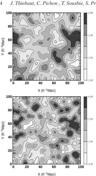
The fact that the non-linearity in the evolution increases chaos is illustrated by Figure 2, where maps of the average density (top panel) and the corresponding Lyapunov exponent λP

(bot-tom panel) are plotted. Each map represents the projection of a

10h−1

Mpc slice from a sample ofS2ata = 0.35. The correlation

between the two maps confirms the dependence of chaos on over density (see also the projections of different realisations of the same halos on Figure 6, where substructures are clearly different even though the shape of main halos remains mostly the same). These results must nonetheless be interpreted with care as the use of a finite sampling grid may bias the measurements. Indeed, consider-ing higher density regions amounts to considerconsider-ing smaller scale re-gions, of order the size of the grid pixels (≈ 1.5h−1

Mpc3), which may affect the measured value ofλP.

3.2 Chaos transition scale

Transition to chaotic behaviour of the density field that started with linear evolution is fundamentally linked to the development of the nonlinearity. Since different scales enter nonlinear regime at dif-ferent epochs, one expects that at a given time there exist a tran-sition scale,Lc, below which variation of the density in pixels of

the sampled field is clearly chaotic. Figure 3 presents the behaviour of the average value ofλP for different perturbation amplitudesA,

as a function of the scaleL. These measurements are derived by

computing the average Lyapunov exponents in pixels on the sam-pled maps shown in figure 2, smoothed using a Gaussian kernel of

1 _{we also considered a128}3_{grid and found no difference in the measured}

exponents.

2

note that the number of pixels above a given threshold is going to depend on redshift, but for the contrasts considered here, the error on the dispersion due to shot noise is always negligible, as we have at least8000 particles

above the highest threshold, at the highest redshift.

−1.0 −0.5 0.0 0.5 1.0 0.00 0.05 0.10 0.15 0.20 0.25 δ ρ/ρ P( δ ρ /ρ ) a=0.1 a=0.15 a=0.20 a=0.25 a=0.30 a=0.35 a=0.40 0.1 0.2 0.3 0.4 0.01 0.02 0.05 ρ/ρ=0.5 S1 ρ/ρ=1 S1 ρ/ρ=1.5 S1 ρ/ρ=2 S1 scale factor a σ 0.1 0.2 0.3 0.4 0.01 0.02 0.05 ρ/ρ=0.5 S2 ρ/ρ=1 S2 ρ/ρ=1.5 S2 ρ/ρ=2 S2 scale factor a σ

Figure 1. top: Evolution of the pixel-averaged PDF of the density

val-ues while sampling S1 on a 643 grid for different values of a ∈ [0.1(light), · · · 0.4(dark)] (only the pixels where ρ/¯ρ > 2 were

con-sidered, whereρ is the cosmic mean density). As expected the full width¯

half max (FWHM) of the distribution increases exponentially with the ex-pansion factor reflecting the chaotic behaviour of the PDF of the density field; middle: temporal evolution of the dispersion in the sampled density field per unit of the mean density, for sub regions ofS1corresponding to

thresholds in overdensityρ/¯ρ of 0.5, 1, 1.5 and 2 respectively as labelled.

The asymptotic merging for different thresholds reflects the fact that at later times, regions of different overdensity levels are all in the nonlinear regime;

bottom: same as middle frame but forS2.

c

0 20 40 60 80 100 0 20 40 60 80 100 1.10 1.70 2.30 2.90 X (h−1_Mpc) Y (h −1 Mpc) 0 20 40 60 80 100 0 20 40 60 80 100 2.30 3.70 5.10 6.50 X (h−1_Mpc) Y (h −1 Mpc)

Figure 2. Logarithm of the projected density of the pixels (top frame) and their associated Lyapunov exponent (bottomframe), for a projected

10h−1_{Mpc sliceS}

2ata = 0.35. The comparison of the two maps

empha-sizes the correlation of the two fields: denser regions have larger Lyapunov exponents. On closer inspection, one may argue that larger Lyapunov expo-nents lie in the outskirts of the denser regions.

FWHML, and considering only the overdense regions (ρ/¯ρ > 1).

Density is computed by making a histogram of particles in the grid using the NGP method, and by smoothing it with a Gaussian kernel afterwards. The measurements are performed at the present time,

a = 1 in S1simulation and ata = 0.4 for S2set.

The plot demonstrates a rather sharp transition to chaotic be-haviour at scales below the critical smoothing lengthLc≃ 3.5h−1

Mpc with Lyapunov exponent increasing for ever smaller scales, whereas on larger scales the Lyapunov exponent is small and con-stant. This behaviour is indicative of theΛCDM background

cos-mology of the standard model. Indeed, in the pure CDM coscos-mology with the critical density of the matter, the gravitational clustering would have continued to escalate to present time and one expect to see Lyapunov exponent falling smoothly to L ≃ 8h−1

Mpc, the present-day nonlinear scale3. In contrast, inΛCDM

cosmol-3

The nonlinear scale is usually defined with top-hat smoothing as

σ2

(RTH) = 1. The FWHM of the Gaussian smoothing filter L that we

use gives similar variance to the top-hat filter atRTH≈ 0.9L. Our

1 2 3 4 5 6 0.0 0.5 1.0 1.5 2.0 2.5 L (h−1Mpc) λP 1/7.5 1/15 1/30 1/60 1/30 2563 1/30 1283cells density fluctuations ρ > <ρ>

Figure 3. Evolution of the average Lyapunov exponent of the pixel

den-sity fluctuations,λP, as a function of the smoothing lengthL for regions

whereρ/¯ρ > 1 and for different amplitudes of the initial perturbations, A

(expressed as a fraction of the initial dispersion amplitude) measured in the setS1. The top dark dashed line corresponds to the setS2forA = 1/30.

The sharp transition nearLsmooth≈ 3.5Mpc/h is exhibited in both

res-olutions. The perturbation amplitude does not affect the result significantly. The difference in time of measurement for theS2 curve (slightly earlier

than the freeze-out time aroundz ∼ 1) may explain small the difference

in the corresponding non linear scale. The bottom light dashed line corre-sponds also toA = 1/30 in S1but measured on a1283grid; it shows that

the exponent is not sensitive to the sampling resolution.

ogy the hierarchical clustering saturates when the dark energy be-gins to accelerate the expansion of the Universe. Numerical simula-tions show that in the standardΛCDM model the clustering largely

ceases by_{z ∼ 1 ((Hatton et al. 2003)). The non-linear scale at} this redshift isL = 3.7h−1

Mpc, which corresponds to the mass scaleM ≈ 2 × 1013

M⊙. The halos of smaller mass collapse en

masse at earlier times passing byz = 1 through a period of

hier-archical mergers with similar-mass halos as well as accretion that contributes to the formation of the chaotic features. Whereas the larger overdense patches, even the rare ones that turned around by

z ∼ 1 and will collapse by the present time, evolve in a quiescent

environment of frozen hierarchy (van den Bosch 2002; Aubert and Pichon 2007). This argues forL ≈ 3.7h−1

Mpc providing the fixed critical length between chaotic and regular regimes for allz < 1,

which is in general agreement with our measurements.

4 LAGRANGIAN EXPONENTS

In the previous section, we studied the development of chaos in the density field of cosmological simulations. We measured the evolu-tion of the variance of this density field on a grid (i.e. at peculiar

Eulerian locations) and showed that chaos tends to be more

pro-nounced in higher density regions as well as on smaller scales. Let us now focus instead on Lagrangian properties of peculiar objects with a physical significance such as dark matter halos or filaments.

tions are normalized toσ(8h−1_{Mpc) = 0.92 which at a = 1 corresponds}

4.1 Inter skeleton distance

Filaments correspond to a central feature of the large scale distri-bution of matter: large void regions are surrounded by a filamen-tary web linking haloes together. Studying the properties of the filaments isn’t an easy thing and one first needs to find a way of extracting their location from a simulation. The skeleton gives a mathematical definition of the filaments as the locus where, start-ing from the filament type saddle points (i.e. those where only one eigenvalue of the Hessian is positive), one reaches a local maxi-mum of the field by following the gradient. This is equivalent to solving the equation:

dx

dt ≡ v = ∇ρ , (2)

for x, whereρ(x) is the density field, ∇ρ its gradient, and x the

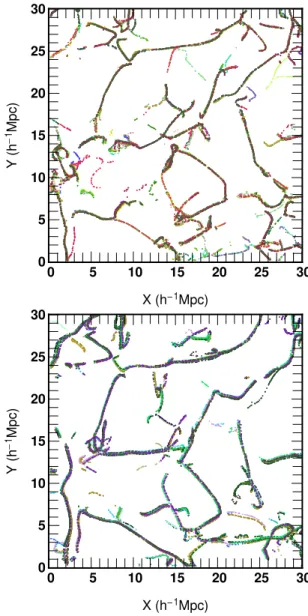
position. Although apparently simple, solving this equation is quite difficult which is why a local approximation was introduced in (Sousbie et al. (2006, 2007)): the local skeleton. One can show that, up to a second order approximation, solving Equation (2) is equivalent to finding the points in the field where the gradient is an eigenvector of the Hessian matrix together with a constraint on the sign of its eigenvalues. This approach leads to a system of two differential equations, solved by finding the intersection of two iso-density surfaces of some function of the iso-density field and its first and second derivatives. This procedure is very robust and allows for a fair detection of the dark matter filaments. Figure 4 displays the skeleton of different realisations ofS2ata(t) = 0.1 (top) and

a(t) = 0.4 (bottom). Note that the dispersion of the skeleton

loca-tion has increased with the scale factor. Using the method described in (Sousbie et al. (2006, 2007)), the local skeleton provides a list of small segments. In order to measure the distance between two skeletons, for each segment, the distance to the closest segment in the other skeleton is computed leading to the PDF of this distribu-tion. The mean distance between the two skeletons is set to the po-sition of the first mode of their inter-distance PDF (See also Caucci et al. (2008)). We then define a mean inter-skeleton distance among all the realisations within a set as the arithmetic average of their pairwise distances. This means that the normalized inter-skeleton distance,hDi /L0, is our measure of the dispersion in the skeleton

location. It is a Lagrangian property since it follows the flow. Its evolution as a function of the scale factor is plotted on Figure 5 for different smoothing lengthsL0, forS2(top) andS1(bottom). The

smoothing operation is achieved, as previously, by convolving the density field with a Gaussian kernel of FWHML0, ranging from

L0 = 1.2 h−1Mpc (3 pixels) up to L0 = 3.5 h−1Mpc (9

pix-els). It is clear that whatever the smoothing scale or the resolution used, the evolution of the dispersion is linear with the scale factor. A shift in the skeleton of the initial conditions will evolve linearly with time and not exponentially: the skeleton at present time won’t be affected very much. There is no chaotic drift of the position of the skeleton and thus no chaos in the evolution of the cosmic web. Note nonetheless that the smaller the smoothing length, the stronger the increase ofhDi /L0. This implies that smaller scales

are more sensitive to initials conditions, which is confirmed by the fact thathDi /L0 is larger for lower values of L0, whatever the

value ofa.

4.2 Positions of halos

Turning to stochasticity on smaller scales in a Lagrangian frame-work (i.e. ignoring the absolute shift in position relative to a fixed

Figure 4. The local skeletons of the different realisations ofS2, computed

ata(t) = 0.1 (top) anda(t) = 0.4 (bottom) and for a smoothing length

L0 = 1.2h−1Mpc. Each figure corresponds to the projection of a10h−1

Mpc thick slice. Each color represents a different realisation of the simula-tion, the color coding is not consistant between the top and the bottom pan-els. The dispersion in the position of the skeletons appears to have grown froma(t) = 0.1 to a(t) = 0.4.

frame), let us define a matching procedure to identify structures in different runs. haloes are first identified using the FOF algorithm (Davis et al. (1985); Suginohara and Suto (1992)) with a percola-tion length of0.25h−1

Mpc forS1 and0.5h−1Mpc forS2

corre-sponding to0.2× mean interparticular distance. In order to tag

dif-ferent FOF haloes in difdif-ferent realisations as counterparts, all par-ticles of a given halo are matched in another realisation using their initial index (Figure 6). The halo of the other simulation containing most of these particles is tagged as its counterpart. The procedure is carried over all pairs of simulations, allowing the measurement of the variation in the halo properties like their spins, their positions, their velocity dispersion tensors or their masses.

As shown on Figure 6, the haloes locations seem relatively insensitive to small changes in the initial conditions. The evolu-tion of the mean distance between a halo in a given simulaevolu-tion and the same halo in another realisation is linear, as for the skeleton,

c

0.1 0.2 0.3 0.4 0 20 40 60 80 100 0.1 0.2 0.3 0.4 0 20 40 60 80 100 <D>/L0 L0=1.17 L0=1.95 L0=2.73 L0=3.51 S2 scale factor a <D>/L0 L0=2.73 L0=3.51 S1

Figure 5. The normalized mean distance,hDi /L0, between the skeletons

ofS2(top) andS1(bottom) as a function of the scale factor and for different

values of the smoothing length,L0 inh−1 Mpc. Because of the lack of

accuracy at smaller scales, only the larger smoothing lengths are represented forS1. At these resolutions, the two sets agree. The cosmic web dispersion

clearly evolves linearly with time, confirming that chaos is linked to non-linearities.

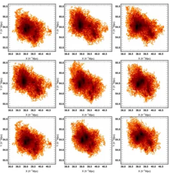
Figure 6. Heaviest cluster (in the X-Y plane in Mpc/h) of 9 realisations

ofS2 atz = 1.5. The position and the global shape of the halo does

not change from one simulation to another, but the substructures are quite different; this is confirmed via automated substructure identification using

ADAPTAHOP.

which confirms the first impressions: no chaos is observed at linear scales and soλQ, the Lyapunov exponent of the inter halo distance,

is null. But the most interesting results involve the substructures. The halo pictured in Figure 6 is a good example of the generic be-haviour. The number of substructures changes from one realisation to another (here, 1 or 2 substructure(s)) and their positions also dif-fer. These results are confirmed by an automated detection of the substructures using ADAPTAHOP (Aubert et al. (2004)). Both the locations and the number of substructures are possibly subject to chaos, but the lack of a cross identification procedure makes it dif-ficult to quantify it and is somewhat beyond the resolution of these sets of simulations (Section 4.3 addresses this problem for the FOF halos). This trend confirms quantitatively the findings of section 3.1 from the point of view of Eulerian estimators which are sensitive to the detailed extension of the distribution of matter within halos: denser regions were found to be chaotic, and will be addressed in more details in Section 4.4 in terms of halo density and velocity moments.

4.3 Connexity and mass of clusters

The connexity of haloes can be defined as follows: considering thepth_{halo, H}r

p, in therthrealisation, its particles are spanned

amongstn haloes in the r′threalisation, and a fractionfpkrr′ (k ∈

1, .., n) of them belong to a halo k among n in the r′threalisation. Hence, its relative connexityCprr′can be defined as:

Cprr′= n X i=1 i   i Y j=1 n X k=j fpkrr′  , (3)

where by constructionCprr′is equal to one if both haloes are

iden-tical in realisationsr and r′

;Cprr′is equal ton if the halo p splits

inton haloes with equal fractions frr′

pk = 1/n in realisation r′,

while preserving continuity when the values offpkrr′differ, see

Ap-pendix A. The mean connexity,C, is obtained by averaging over all

haloes containing more than100 particles in every possible

com-binations of realisations and is a measure of the dispersion of the particles.

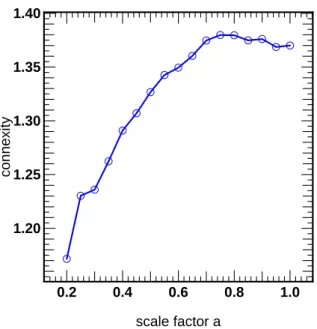
As shown on Figure 7,C increases with the scale factor,

rang-ing from1.17 (i.e., statistically, 90% of the particles belong to a

unique halo in other realisations) to1.37 ( 85%) from a = 0.2 up

toa = 1.0. The connexity clearly does not vary exponentially with

the scale factor : there are statistically no halo fission during evo-lution (thanks to the efficiency of dynamical friction). Moreover, two haloes marginally linked by FOF would almost always end up merging sooner or later. More and more haloes merge at different times in different realisations which is in part due to the fact that some threshold is involved in the FOF algorithm: a precise linking length has to be chosen, inducing the possibility that small changes in particles position can induce significant changes in halo merg-ing time (accordmerg-ing to the FOF definition of a halo). At later times (a > 0.7), the connexity reaches a plateau, which suggests that

when haloes are massive enough (M > Mc, see Section 4.4

be-low), they become insensitive to the merging of lighter ones, since equal mass merging rarely occur belowz = 1. The analysis of the

masses of the haloes shows that there is no sweeping change and so, no obvious evolution of the haloes mass distribution: the associated Lyapunov exponent,λM, is null. The number of different particles

increases with time but the missing particles are replaced by new particles. Thus, the mass stays quite constant even as the connex-ity increases. It follows that the mass function extracted from the

0.2 0.4 0.6 0.8 1.0 1.20 1.25 1.30 1.35 1.40 scale factor a connexity

Figure 7. The haloes average connexity computed over all the realisations

ofS1as a function of the scale factor. While the connexity is not subject to

chaos, its value increases with time. This result can be understood through the difference in merging time of the haloes.

N-body simulations are found to be quite robust with respect to changes in the initial conditions. Although the masses of the haloes are similar in different realisations, some of the particles which compose them may be different, which may generate differences in the physical properties of the haloes. The substructures are dif-ferent (Fig. 6) in their numbers and positions, which is responsible for the Eulerian chaos found in Section 3.2. Let us now re-explore this in a Lagrangian framework.

4.4 Spin Orientation of clusters

The influence of chaos on the spin of haloes is estimated by com-puting the cosine of the angle,θpq, between the spins Jpand Jqof

corresponding haloes in two different realisations p and q:

cos(θpq) =

J_{p· Jq} kJpk kJqk

. (4)

For every bin of mass, a measure of the dispersion,σ, of the

orien-tation is given by the average angle:4

σ = arccos 1 Nc Nc X i=1 cos θpq ! , (5)

where the sum is over all theNcpossible pairwise combinations of

realisations. Note that only bins of masses containing more than 30 haloes have been retained.

Figure 8 displays the exponential growth of this dispersion with time, and shows that the precise value of its associated Lya-punov exponent λσ depends on the selected bin of mass. It also

shows that the exponent does not seem to be sensitive to shot noise, as its value is left unchanged when resolution is increased between

S1andS2.

4

the estimator of the dispersion, Eq. (5) is robust since weighting the sum by the spin parameter yields the same results.

0.2 0.3 0.4 0.5 0.6 0.7 0.8 0.9 3.4 3.5 3.6 3.7 3.8 3.9 4.0 4.1

5.10

_M

<M<6.10

M

5.10

M

<M<6.10

M

256

1.6.10

_Mo<M<2.10

_Mo

scale factor a

ln(

σ

)

Figure 8. Logarithm of the dispersion of the angle between the spin

of one halo ofS1 as a function of the scale factor. Results are

com-puted for different ranges of masses,5 1012_M

⊙¡M¡6 1012M⊙(top) and 1.6 1013_M

⊙¡M¡2 1013M⊙(bottom). For heavier halos the Lyapunov

ex-ponent vanishes. The triangles correspond to the first class of lighter mass, but measured inS2; the exponent remains unchanged which suggests that

particle shot noise is not an issue.

Also, as it is seen in Fig.6, the detailed distribution of satellites within a given cluster varies from one realisation to another; the an-gular momentum orientation (in contrast to say, its modulus or the halo mass) is quite sensitive to the outer region of the distribution. Recall that the spin parameter (i.e. theΛ = J/(√2M V200R200)

(Bullock et al. (2001), Aubert et al. (2004)) of a halo displays no chaotic behaviour. It stays quite constant from a simulation to an-other and the evolution of its dispersion is not exponential.

The measured Lyapunov exponent ranges from 0 to 0.3. The value of the mean dispersion of the orientation of the spin for heav-ier haloes is about 35 degrees (= exp(3.55)). Globally this

sug-gests that the orientation of the spin varies with the tidal field, which in turn depends on the relative position of structures within the environment of the halo.

For lighter haloes, the measured value ofλσ is higher than

for heavier ones (Figure 8) which may be partly explained by the fact that a slight change in a few clumps within the haloes has a larger influence on its spin when they represent a significant frac-tion of it. Faltenbacher & al. (Faltenbacher et al. (2005)) showed that if the lightest halo has a mass less than10% of the mass of the

larger halo, the orientation of the resulting post merging halo will remain statistically the same. In contrast, if its mass is greater than

20% of the more massive halo, the final orientation of the merged

halo depends on the speed vector of the two progenitors. Our re-sults corroborate well their finding since the lightest haloes that are formed by merging of two substructures of comparable masses have chaotic spins (substructures being chaotic, see Section 3 and Figure 6), while heavier ones have spin that are relatively stable with time (they only merge with much smaller haloes). It emerges from these measurements that there is a critical mass,Mc, above

which chaotic behaviour disappears. Haloes heavier than this mass are too heavy to feel the influence of incoming clumps and their

c

0.02 0.04 0.06 0.08 0.10 0.12 0.14 800 1000 1200 1400 1600 Perturbation amplitude A Critical mass M c (10 10 Mo ) spin orientation Mc=2.1013Mo x A0.15

Figure 9. Critical mass,Mc, (in units of1010M⊙) for the spin orientation

as a function of the amplitude of the perturbations,A (in fraction of the

initial dispersion amplitude). It appears thatMc= 2 1013M⊙A0.15. The

larger the amplitude of the perturbation, the heavier the haloes that can be considered stable.

spins are clearly defined. They are therefore not subject to chaos and their Lyapunov exponents are null at the one sigma level, in contrast to lighter ones whose spin are sensitive to the initial con-ditions and whose Lyapunov exponents are positive.

As for the critical smoothing length (see Section 3), we can study the evolution of this critical mass as a function of the ampli-tude,A, of the perturbations. Figure 9 shows this evolution. A good

fit of this transition mass is given byMc= 2 1013M⊙A0.15. The

higher the amplitude of the perturbations, the higher the required time for haloes to have a spin clearly defined. Consequently, the critical mass increases with the perturbation amplitude, and haloes that can be considered stable are heavier. Note that it means that the spin is constant with time but not very reliable since its final orientation depends, in part, on the initial conditions.

4.5 Orientation of the velocity dispersion tensor

The orientation of the velocity dispersion tensor is also a quantity of interest from the point of view of stochasticity since it is related to the shape of the halo via the Virial theorem. The correspond-ing estimator involves computcorrespond-ing the orientation of the eigenvector

V associated to the largest eigenvalue of the velocity dispersion

tensor. As for the orientation of the spin, (Sec. 4.4) the angleθpq

between the eigenvector Vpof the halo in simulationp and its

cor-responding eigenvector Vqin a simulationq is computed as:

cos(θpq) =

V_p.Vq kVpk kVqk

. (6)

For every bin of mass, a measure of the dispersion,σ, is also given

by Equation (5). Once again, only bins of masses containing more than 30 haloes were considered. As shown in Figure 10 this esti-mate is consistent with the exponents of the orientation of the spin: only the lightest masses are sensitive to the initial conditions, while the dispersion of the orientation for the heavier masses is constant (about 40 degrees). The measured Lyapunov exponent,λT, ranges

0.2

0.4

0.6

0.8

1.0

3.6

3.8

4.0

4.2

5.10

_M

<M<6.10

M

5.10

M

<M<6.10

M

256

2.3.10

_Mo<M<2.8.10

_Mo

scale factor a

ln(

σ

)

Figure 10. Logarithm of the dispersion of the angle between the first

eigenvector of the velocity dispersion tensor of the haloes ofS1, as a

function of the scale factor. Results are computed for different ranges of masses:5 1012

M⊙¡M¡6 1012M⊙(top) and2.3 1013M⊙¡M¡2.8 1013M⊙

(bottom). The less massive haloes are more sensitive to the initial condi-tions, the average angle being constant for the heavier ones, about a value of40 degrees. The triangles correspond again to the S2set and shows not

difference. The Lyapunov exponent,λTranges from0 to 0.65.

from 0 up to 0.65 . These results corroborate well those for the spin axis, given that its orientation follows the third eigenvector of the dispersion matrix (i.e. the axis along which dispersion is the small-est). Faltenbacher et al. (2005) showed that the orientation of the principal axis of the halo is correlated with the vector linking the two mergers (i.e. their relative positions) particularly in the case where one of the mergers has a mass smaller than10% of the

sec-ond one. The chaos found at small scales (substructures scale) is once again responsible for the chaos in these geometrical properties of haloes since changing the initial conditions amounts to changing the relative positions of the substructures (see sec.3.1) and thus to changing the orientation of the resulting halo’s dispersion tensor. As for the spin, there is evidence of a critical mass above which chaotic evolution disappears: more massive haloes only merge with lighter ones that do not affect their global properties.

5 CONCLUSION AND DISCUSSION

Let us first emphasize here again that the term chaos is used in this paper in the loose sense, as the age of the universe does not allow for many e-foldings on larger scales. Table 1 summarizes the dif-ferent Lyapunov exponents computed in this paper. As shown in section 3.1 (Figure 3), chaos appears below a critical scale which corresponds roughly to cluster scales. The higher the density, the more chaotic is the corresponding region. We also found that both Lagrangian and Eulerian measurements are consistent: super clus-ters and filaments, whose dynamics is globally linear (large scale structures), are not stochastic: a shift in the initial conditions will increase linearly with the scale factor. By contrast, the distributions of substructures within clusters, whose characteristic size is smaller

than∼ 3.5h−1

Mpc, are governed by non-linear dynamics and may undergo a stochastic evolution for some observables.

Nevertheless, this chaos at substructures scale does not occur for all physical characteristics of the cluster’s halo. A main fraction of particles remains in the same halo from one realisation to an-other, while a difference arises (in part) from the delay in merging times of the substructures. These timing effects are however aver-aged out yielding, to first order, a constant halo mass. It follows that the mass function derived from a simulation is quite consistent from one realisation to another. Similarly, the dispersion of the am-plitude of the total spin of haloes does not increase exponentially with time.

The mass of a given halo is an integrated quantity which does not trace which specific particle entered the FOF halo; similarly, the spin parameter is also an adiabatic invariant, and the trace of the dispersion tensor will relax rapidly to its virial expectation (which is mass dependent) in a few short dynamical times; in contrast, the spin orientation or the orientation of the dispersion tensor will de-pend precisely on the orientation of velocities of the entering parti-cles and has no direct relation to the mass of the halo; it also reflects the initial environment of the proto halo. For instance it has been shown in Sousbie et al. (2007), Aubert et al. (2004) that the halos preferentially anti-align their spin with the axis of the filament in which they are embedded, while we have shown in Section 4.1 that the filament’s locus was not stochastic.

It is possible to recast these interpretations in the context of the peak-patch (Bond and Myers (1996)) description of haloes. In this framework, massive haloes correspond to large quasi spherical patches around density peaks, which non-linear evolution will de-couple from their neighbouring large patches thanks to the cosmic acceleration belowz ∼ 1. Conversely, small haloes correspond

to small typically aspherical peak-patches, and will acquire tidal torques early on which depend specifically on the detailed white noise realisation (which fixes the shape of the peak-patches). In the tidal torque theory, the mass and the spin parameter are essentially integral functions over the volume of these patches, hence will not depend on the initial perturbations, whereas the spin orientation it-self is sensitive to these perturbations, at least at the lower end of the mass spectrum. This is consistent with the low scatter relationship between the spin parameter and the mass (Aubert et al. (2004)).

Thanks to angular momentum leverage, the orientation of haloes is itself affected by stochasticity mostly at small scales, a result which seems insensitive to shot noise as the lyuponov ex-ponents are consistent between setsS1andS2. In fact, as long as

the haloes merging together have similar sizes (masses), the ori-entation of both spin and velocity dispersion tensors is determined by the relative positions and velocities of the two mergers, whose dynamics is non-linear and whose characteristic size is below the critical scale (Figure 3). These results seem robust with respect to resolution.

When the halo is formed and well-isolated by cosmic accelera-tion, it merges only with satellites/substructures whose masses rep-resent a small fraction of the host’s mass. Consequently, their ori-entations are globally preserved after merging, and thus, the chaotic behaviour stops and the dispersion in the orientation remains at the same level (i.e. the resulting average angle is unchanged). Hence, a critical mass can be defined as the mass above which this chaotic behaviour of the orientation stops. The measured value of this crit-ical mass,Mc = 2 1013M⊙A

0.15_{, is just below the scale of}

non-linearity atz ∼ 1 and shows weak dependence on the amplitude

of the added perturbative noise:Mc= 2 1013M⊙A

0.15_{. Although}

some slow increase ofMcwithA is expected since adding power

λ τ (Gyear)

Pixels PDF,λP 0-2.5 3.4-∞

Velocity dispersion tensor,λT 0-0.65 25-∞

Spin orientation,λσ 0.-0.31 75-∞

Inter skeleton distance,λS ∼ 0 ∞

Connexity,λC ∼ 0 ∞

Position of the halos and substructures,λQ ∼ 0 ∞

Mass of the halos,λM ∼ 0 ∞

Spin parameter,λΛ ∼ 0 ∞

Mean dispersion of velocity,λV ∼ 0 ∞

Table 1. Lyapunov exponents of the different observables studied.

Inter-estingly, many global properties of halos do not display chaotic behaviour.

to inhomogeneities shifts the nonlinear scale to higher masses, the details of the dependence require further investigation.

This paper has concentrated on a realisticΛCDM cosmology:

it would also be interesting to rerun this investigation on scale-free power spectra to confirm that the dark energy is indeed responsible for the saturation ofMc. A natural extension of this work, clearly

beyond its current scope, would also involve computing Lyapunov exponents for the properties of substructures within halos (see for instance Valluri et al. (2007)), and parameters corresponding to the inner structure of halos, such as NFW concentration parameter, the phase space densityQ = ρ0/σ3 (Peirani et al. (2006)), the Gini

index or the asymmetry (Conselice et al. (2007)) within the FOF. In closing, the answer to our riddle is that chaos and non-linearities are very strongly linked, and both occur at small scales (substructures scales) though some non linear halo parameters (spin, mass etc...) do not seem to be subject to chaos. While the large scale structures in a simulation (filaments and haloes) are quite robust both in their locus and properties, the distribution of substructures is more sensitive to initial conditions since their num-bers and positions vary when initial conditions vary. This in turn may prove to be a concern when generating zoomed resimulations.

Acknowledgments

We thank the anonymous referee for helpful suggestions, D. Aubert, S. Colombi, and R. Teyssier for fruitful comments during the course of this work, and D. Munro for freely dis-tributing his Yorick programming language and opengl interface (available at http://yorick.sourceforge.net/). This work was carried within the framework of the Horizon project,

www.projet-horizon.fr.

References

D. Aubert and C. Pichon. Dynamical flows through dark mat-ter haloes - II. One- and two-point statistics at the virial radius.

MNRAS , 374:877–909, January 2007.

D. Aubert, C. Pichon, and S. Colombi. The origin and impli-cations of dark matter anisotropic cosmic infall on L* haloes.

MNRAS , 352:376–398, August 2004. c

E. Bertschinger. COSMICS: Cosmological Initial Conditions and Microwave Anisotropy Codes. ArXiv Astrophysics e-prints, June 1995.

J. R. Bond and S. T. Myers. The Peak-Patch Picture of Cosmic Catalogs. III. Application to Clusters. ApJS , 103:63–+, March 1996.

J. S. Bullock, A. Dekel, T. S. Kolatt, A. V. Kravtsov, A. A. Klypin, C. Porciani, and J. R. Primack. A Universal Angular Momentum Profile for Galactic Halos. ApJ , 555:240–257, July 2001. S. Caucci, S. Colombi, C. Pichon, E. Rollinde, P. Petitjean, and

T. Sousbie. The topology of the IGM. MNRAS submitted, 2008. C. J. Conselice, S. Rajgor, and R. Myers. The Structures of Dis-tant Galaxies I: Galaxy Structures and the Merger Rate to z˜3 in the Hubble Ultra-Deep Field. ArXiv e-prints, 711, November 2007.

M. Davis, G. Efstathiou, C. S. Frenk, and S. D. M. White. The evolution of large-scale structure in a universe dominated by cold dark matter. ApJ , 292:371–394, May 1985.

J. Diemand, B. Moore, and J. Stadel. Velocity and spatial biases in cold dark matter subhalo distributions. MNRAS , 352:535–546, August 2004.

A. Faltenbacher, B. Allgood, S. Gottl¨ober, G. Yepes, and Y. Hoff-man. Imprints of mass accretion on properties of galaxy clusters.

MNRAS , 362:1099–1108, September 2005.

J. Goodman, D. C. Heggie, and P. Hut. On the Exponential Insta-bility of N-Body Systems. ApJ , 415:715–+, October 1993. S. H. Hansen and B. Moore. A universal density slope Velocity

anisotropy relation for relaxed structures. New Astronomy, 11: 333–338, March 2006a.

S. H. Hansen and B. Moore. A universal density slope Velocity anisotropy relation for relaxed structures. New Astronomy, 11: 333–338, March 2006b.

S. Hatton, J. E. G. Devriendt, S. Ninin, F. R. Bouchet, B. Guider-doni, and D. Vibert. GALICS- I. A hybrid N-body/semi-analytic model of hierarchical galaxy formation. MNRAS , 343:75–106, July 2003.

H. E. Kandrup. Divergence of nearby trajectories for the gravita-tional N-body problem. ApJ , 364:420–425, December 1990. H. E. Kandrup, B. L. Eckstein, and B. O. Bradley. Chaos,

complexity, and short time Lyapunov exponents: two alternative characterisations of chaotic orbit segments. AAP , 320:65–73, April 1997.

H. E. Kandrup, M. E. Mahon, and H. J. Smith. On the sensitivity of the N-body problem toward small changes in initial condi-tions. 4. ApJ , 428:458–465, June 1994.

H. E. Kandrup and I. V. Sideris. Chaos and the continuum limit in the gravitational N-body problem: Integrable potentials. PRE , 64(5):056209–+, November 2001.

H. E. Kandrup and H. J. Smith. On the sensitivity of the N-body problem to small changes in initial conditions. ApJ , 374:255– 265, June 1991.

H. E. Kandrup and H. J. Smith. On the sensitivity of the N-body problem to small changes in initial conditions. II. ApJ , 386: 635–645, February 1992.

H. E. Kandrup, H. J. Smith, and D. E. Willmes. On the sensitivity of the N-body problem to small changes in initial conditions. III.

ApJ , 399:627–633, November 1992.

J. F. Navarro, C. S. Frenk, and S. D. M. White. A Universal Den-sity Profile from Hierarchical Clustering. ApJ , 490:493–, De-cember 1997.

S. Peirani, F. Durier, and J. A. de Freitas Pacheco. Evolution of the phase-space density of dark matter haloes and mixing effects

in merger events. MNRAS , 367:1011–1016, April 2006. C. Power, J. F. Navarro, A. Jenkins, C. S. Frenk, S. D. M. White,

V. Springel, J. Stadel, and T. Quinn. The inner structure of

ΛCDM haloes - I. A numerical convergence study. MNRAS ,

338:14–34, January 2003.

H. B. Richer, G. G. Fahlman, R. Buonanno, F. Fusi Pecci, L. Searle, and I. B. Thompson. Globular cluster mass functions.

ApJ , 381:147–159, November 1991.

L. V. Sales, J. F. Navarro, M. G. Abadi, and M. Steinmetz. Satel-lites of simulated galaxies: survival, merging and their relationto the dark and stellar haloes. MNRAS , 379:1464–1474, August 2007.

J. A. Sellwood and A. Wilkinson. Dynamics of barred galaxies .

Reports of Progress in Physics, 56:173–256, February 1993.

I. V. Sideris and H. E. Kandrup. Chaos and the continuum limit in the gravitational N-body problem. II. Nonintegrable potentials.

PRE , 65(6):066203–+, June 2002.

T. Sousbie, C. Pichon, S. Colombi, D. Novikov, and D. Pogosyan. The three dimensional skeleton: tracing the filamentary structure of the universe. ArXiv e-prints, 707, July 2007.

T. Sousbie, C. Pichon, H. Courtois, S. Colombi, and D. Novikov. The 3D skeleton of the SDSS. ArXiv Astrophysics e-prints,

February 2006.

V. Springel, N. Yoshida, and S. D. M. White. GADGET: a code for collisionless and gasdynamical cosmological simulations. New

Astronomy, 6:79–117, April 2001.

L. E. Strigari, J. S. Bullock, M. Kaplinghat, J. Diemand, M. Kuhlen, and P. Madau. Redefining the Missing Satellites Problem. ApJ , 669:676–683, November 2007a.

L. E. Strigari, J. S. Bullock, M. Kaplinghat, J. Diemand, M. Kuhlen, and P. Madau. Redefining the Missing Satellites Problem. ApJ , 669:676–683, November 2007b.

T. Suginohara and Y. Suto. Properties of galactic halos in spatially flat universes dominated by cold dark matter - Effects of nonva-nishing cosmological constant. ApJ , 396:395–410, September 1992.

M. Valluri, I. M. Vass, S. Kazantzidis, A. V. Kravtsov, and C. L. Bohn. On Relaxation Processes in Collisionless Mergers. ApJ , 658:731–747, April 2007.

F. C. van den Bosch. The universal mass accretion history of cold dark matter haloes. MNRAS , 331:98–110, March 2002. M. L. Weil, V. R. Eke, and G. Efstathiou. The formation of disc

galaxies. MNRAS , 300:773–789, November 1998.

Q. Zhang and S. M. Fall. The Mass Function of Young Star Clus-ters in the “Antennae” Galaxies. ApJL , 527:L81–L84, December 1999.

APPENDIX A: CONNEXITY

Let us consider a halo,H, split into n parts, Pn

i, i 6 n, with a

fraction,fi, of its particles in each of them, the indices i being

sorted following the decreasing values offi(fi > fjifi < j).

A measureCnof the connexity ofH should indicate the number

of clumps into which it was split, this number does not necessarily have to be an integer, depending on the fraction of the mass ofH

that went into eachPin. For instance, ifn = 2, we want to obtain

C2 = 2 when f1 = f2 = 1/2 and C2 → 1 when f1 → 1 and

f2 = 1 − f1 → 0; as the indices are sorted, 0 < f2< 1/2. So, in

this case, we could write the connexity ofH as:

Now, considering thatH was split into 3 parts P3

i, then0 <

(f2+ f3) < 2/3 and 0 < f3 < 1/3. So C3′ = 2 + 3f3 → 2

iff3 → 0 and C3′ → 3 when f3 → 1/3. It follows that C3′′ =

(f2+ f3)C3′ → 2 when f2→ 1/3 (which implies that f3→ 1/3)

and thatC′′

3 → 0 when f2→ 0 (which implies that f3 → 0 also).

So

C3= 1 + (f2+ f3)(2 + 3f3) (A2)

has the right properties to represent the connexity of a halo split into3 parts. Hence, by generalizing recursively this formula, we

obtain:

Cn = 1 + (f2+ · · · fn) [2 + (f3+ · · · fn) [· · · [n − 2+ (A3)

(fn−1+ fn) [(n − 1) + nfn]] · · ·]] , (A4)

which can be developed as:

Cn = 1 + 2(f2+ · · · fn) + 3(f2+ · · · fn)(f3+ · · · fn) + (A5) · · · + n(f2+ · · · + fn)(f3+ · · · + fn) · · · (fn) , (A6) = n X i=1 i   i Y j=1 n X k=j fk  , (A7)

which corresponds to Eq. (3). Note that by construction, the braket in Eq. (A7) is smaller than1/i, so that Cnis always smaller or

equal ton.

c