Physical conditions of the interstellar medium in high-redshift submillimetre bright galaxies

(1)

HAL Id: tel-01661478

https://tel.archives-ouvertes.fr/tel-01661478

Submitted on 12 Dec 2017

HAL is a multi-disciplinary open access archive for the deposit and dissemination of sci-entific research documents, whether they are pub-lished or not. The documents may come from teaching and research institutions in France or abroad, or from public or private research centers.

L’archive ouverte pluridisciplinaire HAL, est destinée au dépôt et à la diffusion de documents scientifiques de niveau recherche, publiés ou non, émanant des établissements d’enseignement et de recherche français ou étrangers, des laboratoires publics ou privés.

Physical conditions of the interstellar medium in

high-redshift submillimetre bright galaxies

Chentao Yang

To cite this version:

Chentao Yang. Physical conditions of the interstellar medium in high-redshift submillimetre bright galaxies. Astrophysics [astro-ph]. Université Paris Saclay (COmUE); Académie chinoise des sciences (Pékin, Chine), 2017. English. �NNT : 2017SACLS361�. �tel-01661478�

(2)

Physical conditions of the

interstellar medium in high-redshift

submillimetre bright galaxies

Thèse de doctorat de University of the Chinese Academy of Sciences

et de l'Université Paris-Saclay, préparée à l’Université Paris-Sud

École doctorale n°127 Astronomie et Astrophysique d’Île-de-France :

Institut d'Astrophysique Spatiale (IAS),

Purple Mountain Observatory (PMO)

Spécialité de doctorat : Astronomie et astrophysique

Thèse présentée et soutenue à Nanjing, le 22 Septembre 2017

Chentao YANG

Composition du Jury :

M. Guillaume PINEAU DES FORETS

PREM, Université Paris-Sud Directeur de thèse

M. Yu GAO

Astronome, Purple Mountain Observatory, CAS Co-Directeur de thèse

M. Marian DOUSPIS

Astronome, Université Paris-Sud Président

M. Yong SHI

Professeur, Nanjing University Examinateur

M. Hongchi WANG

Astronome, Purple Mountain Observatory, CAS Examinateur

M. Johan RICHARD

Astronome, Observatoire de Lyon Rapporteur

M. Qiusheng GU

Professeur, Nanjing University Rapporteur

M. Alexandre BEELEN

Astronome, Université Paris-Sud Invité

M. Alain OMONT

Directeur de Recherche, Institut d'Astrophysique de Paris Invité

NNT

:

2

0

1

7 SAC

L

S3

6

1

(3)

(4)

Acknowledgements

Without the unconditionally support of my parents and friends, I would never have the chance to treat astronomy as a career to pursue.

It is my supervisors: Alain Omont, Yu Gao and Alexandre Beelen who guide me through the mist. Yu helped me entering the world of submm/mm astronomy. Alexandre is always happy to answer all of my questions and gives me new insights into data reduction and analysis. I would like to give my special thanks to Alain who helped me a lot not only in my daily life during my stay in France, but also being a model of a hardworking astronomer with an incredible amount of energy and enthusiasm in astrophysics. I always feel grateful that he pays attention to my every each idea, and gives me helpful advice. It’s a great honour for me to pursue astronomical research with such a legendary figure.

My friends at Purple Mountain Observatory are great treasures to me. They are the people who support me and help me even with trivial matters. They include Hongjun Ma, Zhiyu Zhang, Daizhong Liu, Fangxia An, Yuxiang Gao, Kexin Guo, Qinghua Tan, Ao Zhao, Xuejian Jiang, Yinghe Zhao, Cong Ma, Zhangzheng Wen, Xiaolong Wang, Lijie Liu, Qian Jiao, En Chen, Qianru He, and many others. Zhiyu’s passion in astronomy inspires me as always. I have also learned a lot from them, such as Daizhong’s circumspection and Fangxia’s diligence. The "star formation in galaxies" group is like a big happy family. And I treasure the time spent with it.

I also enjoy the two years that I spent at IAS in Orsay a lot. The people are friendly there and treated me very well, and I had a great time with all the other PhD students and postdoc there, including Jean-Baptiste, Raoul, Lapo, Clara, Guillaume, Cristiano, Gururaj, Samantha, Amine, Benjamin, Lucie, David and many others. I miss the movie nights with pizzas, and the sushi weekends. I would also like to thank the staff/professors in the MIC group: Mathieu, Nabila, Bruno, Hervé, Nicole and Marian. The administrative members at IAS: Véronique and Patricia also helped me a lot during the two years. I had a great time in Paris with friends from the CNRS French course, especially Yusuke Tanimura, Jerry Yang and Rasa Lk, with whom I was enjoying Paris. I would also like to thank them for sharing the memories.

As last, I also thank my collaborators who have enlightened discussions with me and help me to finish the scientific projects that I worked on: Roberto Neri, Pierre Cox, Eduardo González-Alfonso, Matthew Lehnert, Raphaël Gavazzi, Melanie Krips, Iván, Rob Ivison and many others in the Herschel-ATLAS team. I would like to give my special thank to Roberto who shared his great knowledge of millimetre interferometry with me, to Eduardo with his great expertise in molecular astronomy, and to Raphaël who shared his expertise in gravitational lensing.

(5)

(6)

Résumé

La découverte à l’aide de caméras submillimétriques, d’une population de galaxies submillimétriques (SMGs) obscurcies par la poussière à grand décalage spectral redshift (z), a révolutionné notre connais-sance de l’évolution des galaxies et de la formation stellaire dans les conditions physiques extrêmes. Ces galaxies ultra-lumineuses infrarouges (ULIRGs) renferment les flambées de formation stellaire (‘starburst’) les plus intenses dans l’Univers, avec des taux de formation stellaire dépassant 1000 M_⊙/an, approchant donc la limite de stabilité par pression de radiation d’Eddington. La particularité du domaine millimétrique /submillimétrique et de leur distribution spectrale d’énergie (SED) dans l’infrarouge lointain permet de les étudier avec une bonne sensibilité pour toute la gamme de décalages spectraux de 1 à 6. Elles sont consid-érées comme les progéniteurs des galaxies actuelles les plus massives. Les modèles théoriques d’évolution de galaxies ont été remis en question par la très grande densité observée de ces SMGs à très grand décalage spectral. Les grands relevés extra-galactigues récemment effectués, tels que Herschel-ATLAS et HerMES, en ont découvert des centaines de milliers, ouvrant de nouvelles opportunités pour observer ces objets, leurs groupements et leurs connections avec les grandes structures de l’Univers.

La taille de ces échantillons permet d’y trouver des objets singuliers très rares. C’est le cas de celles de ces SMGs très lointaines (environ une sur mille) qui sont fortement lentillées gravitationnellement par un objet massif (déflecteur) à distance intermédiaire. Dans la grande majorité des cas ces déflecteurs sont des galaxies massives elliptiques assez lointaines à décalage spectral compris entre environ 0.2 et 1.2. L’intérêt de telles lentilles gravitationnelles est de produire à la fois une amplification substantielle de la luminosité apparente de la SMG lointaine, par un facteur typiqueµ ∼ 5–15, et une dilatation de ses dimensions par un facteur ∼pµ. L’accroissement substantiel de sensibilité et de résolution angulaire effectives qui en résulte est un énorme atout pour l’étude de ces objets et spécialement de leur milieu interstellaire et de leurs flambées de formation stellaire. Mais la complexité des effets de lentille gravitationnelle impose la construction de modèles élaborés pour reconstruire l’image réelle de la source lointaine à partir de l’image lentillée observée.

Nous avons utilisé cette puissance des lentilles gravitationnelles pour une étude systématique du milieu interstellaire des flambées de formation stellaire des SMGs, basée principalement sur un nouveau critère, l’intensité des raies d’émission submillimétrique de la vapeur d’eau. Nos études antérieures avaient en effet montré d’une part que ces raies submillimétriques pouvaient être les plus intenses après celles de CO dans les SMGs à grand décalage spectral z, et d’autre part qu’elles constituaient un puissant diagnostic des conditions dans les ULIRGs locales, dont on pense qu’elles sont le meilleur modèle (réduit) local des SMGs à grand z. Cette étude est centrée sur l’observation des raies de H2O dans un échantillon

substantiel de SMGs effectuée à l’Institut de radioastronomie millimétrique (IRAM) avec l’interféromètre millimétrique NOEMA. Nous lui avons adjoint une étude systématique des raies de CO dans les mêmes sources à l’IRAM/30m pour un diagnostic complémentaire, ainsi que celle de H2O+, clé de la chimie de

(7)

vi

ALMA ou NOEMA pour sonder la structure du gaz moléculaire et de la flambée de formation stellaire dont il est le siège.

Nous avons donc sélectionné un échantillon de 16 SMGs fortement lentillées, extrêmement brillantes, en choisissant celles dont les densités de flux submillimétrique sont les plus élevées dans les 300 deg2 des champs Nord et équatoriaux du relevé Herschel-ATLAS. Leur observation à l’aide de l’interféromètre millimétrique NOEMA nous a permis de détecter dans chacune au moins une raie submillimétrique de H2O, déplacée dans une fenêtre atmosphérique millimétrique. Leur forte intensité confirme que ces raies

sont les raies submillimétriques les plus brillantes dans ces objets après celles de CO. Nous avons trouvé une corrélation linéaire forte entre la luminosité de H2O et la luminosité infrarouge totale. Cela indique

le rôle important du pompage infrarouge lointain dans l’excitation des raies de l’eau. En utilisant un modèle de pompage infrarouge, nous avons obtenu les propriétés physiques du gaz et de la poussière interstellaires ainsi que l’abondance de H2O. Nous avons montré que les raies de H2O tracent un gaz chaud

et dense, baignant dans un champ de rayonnement infrarouge lointain intense, émis par les flambées extrêmes de formation stellaire.

Plusieurs raies de H2O+ont également été détectées dans trois de ces SMGs dans la bande de fréquence

des observations de NOEMA. Elles montrent qu’il existe une corrélation étroite entre les luminosités des raies de H2O et H2O+, qui s’étend des ULIRGs locales aux SMGs à très grand z. Le rapport élevé de

flux H2O+/H2O suggère que des rayons cosmiques très intenses, produits dans les fortes flambées de

formation stellaire, sont probablement à l’origine de la chimie de l’oxygène dans ce milieu en y formant abondamment les molécules H2O et H2O+.

Nous avons observé en complément de multiples transitions rotationnelles de la molécule CO dans chacune de cette quinzaine de SMGs, avec le spectromètre millimétrique multi-bande EMIR du télescope de 30m de l’IRAM. Nous avons ainsi établi la distribution spectrale de l’émission dans les raies de CO de ces galaxies. Elle semble présenter une certaine similitude avec celle des ULIRGs locales. Nous avons mis en évidence un effet significatif de lentillage différentiel qui pourrait entraîner une sous-estimation de la largeur de raie d’un facteur allant jusqu’à 2. A l’aide d’une modélisation de type LVG et en utilisant une approche bayésienne, nous avons estimé la densité et la température du gaz, ainsi que sa densité de colonne dans la molécule CO. Nous avons ensuite mis en évidence une corrélation entre la pression thermique du gaz et l’efficacité de la formation stellaire. Nous avons également étudié les propriétés globales du gaz moléculaire et sa relation avec la formation d’étoiles ainsi que le rapport masse de gaz sur poussière et le temps d’épuisement du gaz. La détection de raies du carbone atomique neutre [CI] dans

ces SMGs à grand décalage spectral y a étendu la corrélation linéaire, connue pour les galaxies locales, entre luminosité des raies de CO et de [CI]. Enfin, nous avons comparé les largeurs de raie de CO et H2O et

constaté qu’elles étaient en bon accord. Cela suggère que les régions émettrices soient co-spatiales. Afin de comprendre les propriétés des émissions moléculaires dans ces sources, et plus généralement, leur structure et leurs propriétés dynamiques, il est crucial d’en acquérir des images à haute résolution angulaire. Nous avons donc observé deux de ces sources avec les interféromètres ALMA ou NOEMA en configuration étendue des antennes. Grâce à une modélisation du lentillage de ces sources, ces données nous ont permis de reconstituer la morphologie intrinsèque de la source. Nous avons ainsi mis en évidence que la région de l’émission de la poussière relativement froide qui évacue l’énergie considérable de la flambée stellaire, a une plus petite taille en comparaison de celle du gaz CO et H2O, tandis que les régions

d’émission de ces deux dernières molécules sont de taille similaire. En ajustant le modèle dynamique de la galaxie aux données CO, nous avons montré qu’elle peut être modélisée par un disque en rotation, duquel nous avons pu déduire la masse dynamique projetée et le rayon effectif. Ces études nous ont également

(8)

vii

permis de confirmer la détection à grand z de l’isotopologue rare H18₂ O dans ces deux sources, montrant que de futures études de cette molécule avec ALMA dans de telles galaxies lentillées devraient apporter des informations intéressantes sur la nucléosynthèse de18O à grand z.

Avec ALMA et la future extension de NOEMA, nous pourrons étendre ce genre d’observations, spéciale-ment à haute résolution angulaire, à un plus grand nombre de SMGs à grand décalage spectral fortespéciale-ment amplifiées (et même à des SMGs non lentillées grâce à la sensibilité d’ALMA), afin d’étudier divers traceurs du gaz moléculaire et de comprendre les conditions physiques et chimiques du milieu interstellaire et leur relation avec la formation des étoiles.

(9)

(10)

Chapter 1 Introduction

That destructive monster of a hundred heads, im-petuous Typhon. He withstood all the gods, hissing out terror with horrid jaws, while from his eyes light-ened a hideous glare.

Prometheus Bound by Aeschylus

1.1 Discoveries of the submillimetre-bright galaxies at high-redshift

Deep submillimetre (submm) imaging using SCUBA/JCMT (Holland et al.,1999) of the Hubble deep and blank field has revealed a new population of galaxies releasing massive amount of energy through the Rayleigh-Jeans side of the blackbody emission of the dust (Barger et al.,1998;Hughes et al.,1998;Smail et al.,1997). This discovery as a major breakthrough in the late 1990s expanded our understanding of the big picture of galaxy formation and evolution and opened a new observation window in submm bands.

Barger et al. 1998 Hughes et al. 1998

The discovery of SubMillimeter Galaxies (SMGs) SCUBA 850 micron

Fig. 1.1 Left: First image of SMGs detected by SCUBA-850µm imaging reported byBarger et al.(1998);

Hughes et al.(1998);Smail et al.(1997). Right: The James Clerk Maxwell Telescope (Credit: www.roe.ac.uk) on which the SCUBA instrument is mounted.

(15)

2 Introduction

Template:

Arp

220

10-4 ₁₀-3 ₁₀-2 ₁₀-1 ₁₀0 ₁₀1 ₁₀2 ₁₀3 103 102 101 100 10-1 10-2 10-3 10-4 Wavelength [mm] F lu x d e n s it y [m Jy ] z = 0.5 z = 1 z = 2 z = 4 z = 6 z = 10

Fig. 1.2 The observed spectral energy distributions (SED) of Arp 220 from the optical to the radio wave-lengths as seen at different redshifts. The optical/NIR band is shown in blue while the submm/mm band is shown in green.

Since the initial discovery of SMGs at 850µm with SCUBA at the end of last century, a large num-ber of studies have been conducted, and mostly with the help of interferometric observation in order to pinpoint the number counts and the positions of the SMGs (Blain et al.,2002;Casey et al.,2014;Smolˇci´c et al.,2012). The success of SMG observations is also partially due to the neg-ative K -correction, especially for the studies con-ducted at ∼ 1 mm bands. As illustrated in Fig.1.2, with increasing redshift, spectral energy distribu-tions (SED) of Arp 220 shifts towards longer wave-length while its total flux decreases and the emis-sion peak also shifts in the same direction. As a result, the flux density at ∼ 1 mm bands prac-tically does not vary with redshifts. Chapman et al.(2005) carefully studied the properties of this 850µm-selected SMG population and concluded

that those with S850µm> 1 mJy contribute a significant fraction to the cosmic star formation around z = 2–3,

i.e. ≳10%. Fig1.3shows the evolution of the contribution of different types (defined by their far-IR luminosity) of galaxies to the cosmic star formation along different redshifts. The importance of the most luminous galaxies in the far-IR is clearly increasing with redshift. Several other works have also confirmed that SMGs play a key role in the cosmic star formation at high-z (e.g.Michałowski et al.,2017;Murphy et al.,2011;Swinbank et al.,2014). For the ULIRGs studied with a median redshift of 2.2, it can be > 65% according toLe Floc’h et al. 2005andDunlop et al. 2017(see also ALMA works byAravena et al. 2016a;

Dunlop et al. 2017;Karim et al. 2013;Oteo et al. 2016; andCasey et al. 2014for redshift distributions of SMGs selected at 850–870µm by SCUBA/LABOCA and at 1.1 mm by AzTEC). In the redshift range around z = 1 to z = 3, also known as the epoch of galaxy assembly, the cosmic star formation rate density reaches its peak (as shown in the left panel of Fig.1.3,Lilly et al. 1996;Madau et al. 1996, see alsoMadau & Dickinson 2014for a review). Around half the stars in the present-day Universe have formed around this period (Shapley,2011, and the references within).

This new population of dusty starbursts are the strongest starbursts throughout the star formation history of our Universe. The most luminous ones with infrared luminosities integrated over 8–1000µm

LIR∼ 1013L⊙, and star formation rate (SFR) around 1000 M⊙yr−1, approach the limit of maximum

star-bursts (Barger et al.,2014). These submm bright galaxies (SMGs, see reviews byBlain et al.,2002;Casey et al.,2014) are the veritable “monsters” in our universe just like the Typhon in ancient Greek myth. Even comparing with the local ultra-luminous infrared galaxies (ULIRGs, whose LIRequals a few 1012L⊙), they

are somewhat more luminous (Tacconi et al.,2010). Their extremely intense star-forming activity indicates that these “Typhon”-like galaxies generating enormous energy at far-infrared (far-IR) are in the critical phase of rapid stellar mass assembly as mentioned above. Although there are pieces of evidence of a diverse population of the SMGs (e.g.Banerji et al.,2011), they are believed to be the progenitors of the most massive galaxies today (e.gLonsdale et al.,2006;Simpson et al.,2014).

To understand such a cosmic star formation history shown in Fig.1.3, compatibility with the galaxy formation models in the context ofΛCDM (the hierarchical cold dark matter halo model) is needed. Therefore, under the big picture of galaxy formation and evolution, it is important to understand the

(16)

1.2 Studying the high-redshift SMGs with various molecular gas tracers 3

epoch of galaxy assembly

Fig. 1.3 The history of cosmic star formation and the contribution from various types of galaxies. Left: the evolution of cosmic star formation density, defined by the mass of stars formed per year per comoving volume in cubic Mega-parsec, along the lookback time (redshifts), adapted fromMadau & Dickinson

(2014). Right: the evolution of the contribution from different types of galaxies to the cosmic infrared luminosity, which serves as a proxy of star formation rate. This figure is adapted fromMagnelli et al.(2013).

extreme star-forming activity within SMGs through studying their molecular gas content which serves as the raw ingredient for star formation, especially those at the peak of the star formation history (i.e. z ∼ 2–3,

Madau & Dickinson,2014). Moreover, theoretical models of galaxy evolution have been challenged by the observed large number counts of high-z SMGs (e.g.,Casey et al.,2014). Nevertheless, due to their great distances, the number of well studied high-z SMGs is limited (see reviews byCarilli & Walter 2013;

Solomon & Vanden Bout 2005) and the observations were mostly achieved through a few cases of strong gravitation lensing, including IRAS F10214+4724 (Ao et al.,2008), APM 08279+5455 (Weiß et al.,2007), Cloverleaf (Bradford et al.,2009), SMM J2135-0102 (Danielson et al.,2011) and in the weakly lensed SMG, HFLS3 at z = 6.34 (Cooray et al.,2014;Riechers et al.,2013). Therefore, studies of the star formation properties of such a population of galaxies based on a fairly large sample is needed.

1.2 Studying the high-redshift SMGs with various molecular gas tracers

1.2.1 Molecular gas in galaxies

Although, the interstellar medium (ISM), that is, the gas and dust between stars, makes only a small fraction of the total baryonic content (its mass is ∼ 10% of the total mass of a galaxy), it plays an essential role in shaping a galaxy that we can observe, by circling the fuel and ashes of the death and birth of stars and transferring energies into different phases within a galaxy as shown in Fig.1.4. It serves as the key framework of star formation (e.g.Omont,2007). For the gas phase ISM, it is mostly made of ions, atoms and molecules. In the Milky Way, the ionised gas mostly consists of ionised hydrogen (H II) that contributes to 23% of the total gas mass, while the neutral gas, mostly neutral hydrogen (H I) makes a fraction of 50% and the molecular gas, mostly H2gas, makes a fraction of 16% (e.g.Draine,2011). The fraction of the

molecular gas can be much higher than that of the Milky Way in high-z star forming galaxies (e.g.Tacconi et al.,2013). The physical conditions of the ISM itself exhibit a large range of kinematic temperature (Tk) and volume density (n), so that the ISM is presented in different phases. The hot ionised gas, with n < 0.01 cm−3_{and T}

k> 105K, fills approximately half of the ISM volume in our Galaxy. The warm ionised

(17)

4 Introduction

while the cool neutral atomic gas has n ∼ 30 cm−3and Tk∼ 100 K. For the molecular gas, it usually resides in

two environments: the diffuse molecular gas with n ∼ 100 cm−3and Tk∼ 10–50 K and the dense molecular

gas with n ∼ 103–106cm−3and Tk∼ 10–50 K (e.g.Draine,2011;Tielens,2005). Not only the ISM shows

a large variety of its physical conditions, but it also has a complicated dynamics, which can transfer matter and energy between the different phases. These various processes are thus tightly linked with the ecosystem of the galaxy (Fig.1.4).

Among the different phases of the ISM, the dense molecular gas is usually in form of gravitationally bound clouds that can eventually proceed to star formation. Thus, it serves as a key for us to understand star formation in galaxies. According to the solar element abundances, hydrogen is above≳103times more abundant comparing with heavy elements (except for helium which is about 10 times less abundant than H). This makes the abundance of H2to be orders of magnitude larger than that of the other molecules.

Nevertheless, the direct observation of H2is difficult in the molecular gas phase ISM because H2has no

dipole moment1and therefore very weak rotational transitions. Thus, the observation of the molecular phase of the ISM much relies on molecular species with non-zero dipolar moments, especially the12C16O (we use CO if not otherwise specified in this thesis) molecule. We will further explain the basics of the molecule species and describe their energy levels in the next section.

Fig. 1.4 The life cycle of the ISM (figure adapted fromTielens 2013): gas and dust are ejected by dying starts into the diffuse ISM (stellar ejecta), and by cooling, the neutral gas forms molecular clouds which then proceed to star and planet formation when being gravitationally unstable. Legends show some common gas tracers of different stages of the life-cycle.

1_{If the positive and negative charges of neutral molecule do not completely overlap, the electric dipole moment can be defined}

as a vector pointing from the negative to the positive charge, whose length equals the strength of each charge times the charge

(18)

1.2.1.1 Energy levels of molecules

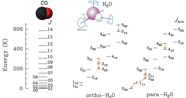
Molecular spectra are unlike atomic ones that can be determined simply by transitions between individual electronic states. They show a complexity because of the extra degrees of freedom coming from vibration and rotation. The electronic transitions of molecules generally emit in the ultraviolet wavelength. For a molecule that transits between specific rotational levels of certain vibration states, the transition is called a ro-vibrational transition. It emits photons in the infrared bands (e.g.Williams & Viti,2014). The most commonly observed transitions belong to the pure rotational transitions that happen between two rotational energy levels within one vibrational state (usually the ground state in the molecular gas phase). Fig.1.5shows the pure rotation energy levels (in the ground vibrational state and the ground electronic state) of the CO and H2O molecules together with their dipole moments. CO is a typical diatomic molecule

while H2O is a non-linear polyatomic molecule. For the latter, the two protons of H2O can either have

antiparallel (“para") or parallel (“ortho") nuclear spins, which makes the transition between para and ortho-H2O impossible. Thus, H2O can be treated as two molecules, e.g. para-H2O and ortho-H2O, as

shown in Fig.1.5.

For diatomic molecule like CO (see Fig.1.5for a sketch of the CO molecule structure), and in the ground vibrational state and the ground electronic state, the rotational energy level is decided by the rotational angular momentum J (energy levels are shown in Fig.1.5). The rotational selection rules for the heteronuclear diatomic molecules are∆J = ±1 (not counting net spin or orbital angular momentum), while the homonuclear diatomic quadrupole selection rules∆J = ±2. As for the case of CO, the J = 1 → 0 transition, i.e. CO(1–0), is at 115.271 GHz (see a list of transitions in Table1.1).

For the polyatomic molecules that include more than two atoms, the situation can be classified into four categories: 1) linear molecules such as HCN, CO2and HCO+; 2) symmetric top molecules such as NH3

and H+₃; 3) spherical tops such as CH4; 4) asymmetric tops such as H2O and H2CO. Using three mutually

orthogonal moments of inertia, Ia, Ib and Ic (a, b and c are three mutually orthogonal axes), one can

describe the state of a polyatomic molecule. Generally, the moment of inertia is defined byP

imir_i2, where

miis the mass of the ithatom at a distance of rifrom the centre of mass.

This can be further simplified for many linear molecules, where the energy levels can be given by

E (J ) = ℏ

2IJ (J + 1), (1.1)

in which I is the moment of inertia and J is the rotational level of the molecule. This means that the heavier molecules (whose values of I are large) will have closer energy levels. Selection rules for this kind of molecule is also∆J = ±1. Taking HCN for example, the J = 1 to ground level J = 0 transition is allowed and can be written as HCN(1–0).

For the case of symmetric top molecules, two of the moments are the same. Thus, either Ia< Ib= Ic

(prolate) or Ia= Ib< Ic(oblate) can describe the state of a molecule. The energy level can thus be written

as E (J , K ) = ℏ 2IaJ (J + 1) + ℏ 2( 1 Ia− 1 Ib )K2, (1.2)

which is characterised by the angular momentum J and its projection on the symmetry axis, i.e. K . The corresponding selections rules are∆K = ±0 and ∆J = ±0,±1.

As for spherical top molecules like CH4, three moments of inertia, Ia, Iband Ic, are equal but have no

(19)

6 Introduction

Another category of molecules, asymmetric tops are nonlinear rotors. The value of Ia, Iband Icare all

different, thus the energy levels are computed using numerical methods. To describe the energy level of such a molecule, one needs the angular momentum J and its projection on the a and c principal axes (see the sketch of H2O molecule in Fig.1.5), Kaand Kc. Accordingly, the energy can be expressed as E (J , Ka, Kc),

and the quantum numbers can be written as JKaKc. The election rules depend on the components of

the permanent dipole momentµ along the principal axes a, b and c: when µa̸= 0, the selection rules

are∆Ka = ±0, ±2, ±4, ..., ∆Kc = ±1, ±3, ±5, ...; when µb̸= 0, the selection rules are ∆Ka = ±1, ±3, ±5, ...,

∆Kc= ±1, ±3, ±5, ...; when µc ̸= 0, the selections rules are ∆Ka= ±1, ±3, ±5, ..., ∆Kc = ±0, ±2, ±4, .... For

all the three cases,∆J = ±0,1. Take the most important asymmetric top molecule, H2O, for example.

The transition of ortho-H2O from energy level 523to 514is allowed, which is written as H2O(523–514),

corresponding to a frequency of 1410.618 GHz. As we mentioned previously, ortho-H2O and para-H2O can

be treated as two molecules. For ortho-H2O, the value of Ka+ Kcis odd, while for the para-H2O, Ka+ Kc is

even.

Fig. 1.5 The energy levels of CO and H2O molecules, together with their quantum numbers J and JKaKc. The upper sketches show the structure of the CO and H2O molecules. The three axes of the H2O molecule

are also indicated. Yellow arrows show the eight brightest H2O rotational lines that are detected in local

galaxies (Yang et al.,2013).

1.2.1.2 Line radiative transfer

The transition between different rotational energy levels of molecules can happen with several processes: mainly interactions with photons and collisions with other atoms, molecules and electrons. In short, the excitation can be either radiative or collisional. Fig.1.6shows a cartoon comparing collisional excitation with radiative excitation. The molecule can jump from a lower rotational energy to a higher one by colliding with another gas particle (mainly H in the atomic gas and H2in the molecular gas) or by a photon with an

energy equal to the energy difference between the two rotational energy levels. Then the molecule can jump back to the lower energy levels by emitting photons. This radiative de-excitation is determined by the Einstein A-coefficient. Take CO molecule for example, the excitation through collisions with H2and

(20)

the following de-excitation can be expressed as:

CO(J−_−0,₁) + H2−−→ CO(J −−2) + H2,

CO(J−_{−2) −−→ CO(J −}_{−1) + hν,} (1.3)

for the collisional processes, and

CO(J−_{−1) + hν −−→ CO(J −}_−2),

CO(J−−2) −−→ CO(J−−1) + hν, (1.4)

for the radiative excitation. The corresponding CO line for Eqs.1.3and1.4is CO(2–1).

Collisional excitation: Excitated to higher Energy through collision.

IR-pumping excitation: Excitated to higher Energy

through absorbing an infrared photon.

Trace Gas

Trace

Radiation

_{Credit: Semenov}

Fig. 1.6 A cartoon showing a comparison between collisional excitation and radiative excitation of a diatomic molecule. The left panel shows the process of excitation and de-excitation while the right panel shows the energy level diagram and the transitions shown in the left panel.

To further quantify the permitted transition between different energy levels, one needs the Einstein coefficients. Taking a two-level system as an example, as shown in Fig.1.7, the upper and lower level energies are EUand EL, respectively. For an atom/molecule transitioning from an upper (U) to a lower (L)

energy state, the spontaneous emission coefficient AULdescribes the photon spontaneous emission rate

per second, while the absorption coefficient BLUand the stimulated emission coefficient BULquantify the

processes of absorption and stimulated emission.

Considering a system with a large number of atoms/molecules, the number of particles per unit volume in the upper energy state U is nUand nLis the number for the particles in the lower state L. Then,

(21)

8 Introduction

A

_UL

B

_LU

E

_U

E

_L

B

_UL

hν

₀

Fig. 1.7 Figure adapted from (Condon & Ransom,2016) showing a sketch of a two-level system (upper level U and lower level L). The three Einstein coefficients are AULfor spontaneous emission, BLUfor absorption,

and BULfor stimulated emission. EUand ELare the upper and lower level energies. hν0is the photon

energy that equals to EU− EL.

because of the balance between emission and absorption, in the absence of collisions we can have

nUAUL+ nUBULu = n¯ LBLUu,¯ (1.5)

in which ¯u is the profile-weighted mean radiation energy density because of the finite width of the

spectral line profile (so that BULu and B¯ LUu equal the average rate per second at which the photons are¯

emitted/absorbed by a single particle). If we consider now the collisional excitation/de-excitation, using the CULand CLUto describe the possibilities of the collisional excitation transition, Eq.1.5becomes

nUAUL+ nUBULu + n¯ UCUL= nLBLUu + n¯ LCLU. (1.6)

For a system that has a well-defined temperature on a scale much greater then the free mean path of a photon, it is said to be in local thermodynamic equilibrium (LTE). That well-defined temperature is the kinetic temperature Tkrelated to the Maxwellian speed distribution of the particles. Nevertheless, in

general, the energy levels will not be in LTE (non-LTE). It is thus instructive to quantify Texby

nU nL ≡ gU gL exp µ −hν0 kTex ¶ , (1.7)

where gUand gLare the statistical weights of the energy states EUand EL, respectively. k is the Boltzmann

constant. Tex quantify the ratio of nU to nL. Observationally, whether the molecular line appears in

absorption or emission depends on the value of the excitation temperature, Texcomparing with the

back-ground temperature Tbg: if Tex> Tbg, the line will be seen in emission and the line appears in absorption

if Tex< Tbg. For collisional excitation, this excitation temperature can depend on the critical density, at

which the excitation balances spontaneous de-excitation, of a particular transition. The critical density can be written as

ncrit,UL≡ AUL

Σi̸=UγUi

, (1.8)

whereγUiis the collision rate coefficient from level U to level i (e.g.Tielens,2005). Table1.1shows the

critical densities (ncrit) of CO lines calculated by assuming a gas temperature Tk= 100 K, an ortho to para

ratio of H2of 3 and an optically thin regime.

A special case of the transition happens when the upper energy level is overpopulated as,

nU nL >

gU gL

, (1.9)

then from Eq.1.7, we can then derive that Tex< 0. This gives a negative net line opacity, namely that the

(22)

stimulated emission of radiation) at radio wavelengths (see reviews by e.g.Elitzur,1992;Lo,2005;Reid & Moran,1981). The most commonly detected astrophysical masers include OH masers and H2O masers.

Table 1.1 Basic information about the CO rotational lines.

Molecule Transition νrest Eup/k AUL ncrit

JU→ JL (GHz) (K) (s−1) (cm−3) CO 1 → 0 115.271 5.5 7.20 × 10−8 _{2.4 × 10}2 2 → 1 230.538 16.6 6.91 × 10−7 2.1 × 103 3 → 2 345.796 33.2 2.50 × 10−6 7.6 × 103 4 → 3 461.041 55.3 6.12 × 10−6 1.8 × 104 5 → 4 576.268 83.0 1.22 × 10−5 _{3.6 × 10}4 6 → 5 691.473 116.2 2.14 × 10−5 6.3 × 104 7 → 6 806.652 154.9 3.42 × 10−5 1.0 × 105 8 → 7 921.800 199.1 5.13 × 10−5 _{1.5 × 10}5 9 → 8 1036.912 248.9 7.33 × 10−5 2.1 × 105 10 → 9 1151.985 304.2 1.00 × 10−4 2.9 × 105 11 → 10 1267.014 365.0 1.34 × 10−4 3.9 × 105

Note: The frequencies (νrest), upper level energies (Eup/k) and Einstein A coefficients are

taken from the LAMDA database (Schöier et al.,2005). The collision rate coefficients are from

Yang et al.(2010). We assume the gas temperature Tk= 100 K, and an ortho-H2to para-H2

ratio of 3 and an optically thin regime for calculating the critical densities here.

To summarise, through observing the multiple transitions of the molecular gas tracers such as CO, one can in principle derive a rich information about the physical conditions of the ISM such as the density and temperature of the molecular gas, if the molecules are collisionally excited. If radiative excitation is involved, one can also infer information about the surrounding radiation fields, by observing the lines. We will further discuss the implications of such kind in high-z SMGs in the next section.

1.2.2 Probing the physical properties of the ISM in high-z SMGs

Because high-z SMGs are highly dust-obscured, it is difficult or impossible in most situations to observe them with optical/near-infrared (NIR) telescopes that probe their stellar content. On the other hand, thanks to the magical power of the negative K -correction (see Section1.1) at submm/mm, the dust continuum emission at submm and molecular lines are the most efficient way to study star formation in high-z SMGs.

Molecular gas serves as the direct fuel of star formation (Leroy et al.,2008;Schruba et al.,2011). The linear correlation found between the dense molecular gas and the star formation rate from the dense cores of galactic clouds (Wu et al.,2005) to ULIRGs (Gao et al.,2007;Gao & Solomon,2004) has shown that the dense molecular phase traced by HCN is directly linked to star formation. Therefore, investigating the molecular gas and dust content in those high-z SMGs is the key to understand the conditions of star formation, the nature of SMGs and how they fit into the big picture of galaxy evolution. Such high-sensitivity observations at submm/mm bands are now technically feasible thanks to the Atacama Large Millimetre/submillimetre Array (ALMA) and IRAM’s northern extended millimetre array (NOEMA) (Fig.1.8). ALMA, currently contains fifty 12 m dishes in the 12-m array and twelve 7 m dishes plus four 12 m dishes in the compact array, provides continuum and spectral line capabilities from ∼ 0.3 mm to 3.6 mm, with

(23)

10 Introduction

angular resolutions from ∼ 0.02" to 3.4". NOEMA, currently contains 9 15 m dishes, equipped with state-of-the-art high-sensitivity receivers, provides continuum and spectral line capabilities from ∼ 0.8 mm to 3.6 mm, with angular resolutions from ∼ 0.4" to 3.6".

ALMA

NOEMA

Fig. 1.8 Photos of ALMA and NOEMA (credit: ESO and IRAM).

Molecular gas tracers are among the most important means through which we understand the nature of these high-z SMGs. The observations of the cool molecular gas traced by low energy levels and low critical density gas tracers, such as low-J lines and the two [CI] fine-structure lines (CI3P1→3P0at 492.2 GHz and

CI3P2→3P1at 809.3 GHz, [CI](1–0) and [CI](2–1) hereafter, respectively) are able to provide a rich set of

information about the galaxies where they reside. Because those molecular gas lines trace the bulk of the total molecular gas of the SMGs, from the emission/absorption line profiles, one can have insights into the dynamics of the galaxies. One can even be able to reveal the kinematical structure of the SMGs given enough spatial resolution (achievable with submm/mm interferometers), e.g. a rotating disk (e.g.Dye et al.,2015) or a dissipative merger system (e.g.Tacconi et al.,2008). With only unresolved single-dish observations, those linewidths can provide estimates of the dynamical masses (Bothwell et al.,2013b, however one needs to assume whether the source is a major merger or a rotating disk, which can lead to very different results).

The flux of the CO(1–0) line is also a powerful/standard tool to derive the total mass of molecular gas in galaxies by assuming that the molecular gas mass is proportional to the luminosity of the CO(1–0) line,

L′_CO(1–0)(in unit of K km s−1pc2) which can be derived followingSolomon & Vanden Bout(2005)

L′_CO(1–0)= 3.25 × 107SCO∆vν−2_obsD2_L(1 + z)−3 (1.10)

where SCO∆v is the velocity-integrated flux in Jy km s−1,νobsis the observed frequency in GHz, DLis the

luminosity distance in Mpc and z is the redshift. The molecular gas mass can then be derived through a conversion factorαCOsuch as MH2= αCOL′CO(1–0), where MH2 is the mass of molecular hydrogen and

(24)

αCOis the conversion factor to convert observed CO line luminosity to the molecular gas mass without

helium correction (this factor may also be written as XCOdepending on the units, seeBolatto et al. 2013

for a review). This method is commonly used in extragalactic studies. Nevertheless, the value of the CO to H2conversion factorαCOappears to be different in various systems. The determination ofαCO

is usually achieved by constraining the dynamical mass from the virial mass, or from the measurement of the H2gas mass byγ-ray observation or by using a gas to dust mass ratio. For normal local galaxies,

the value of this conversion factor measured appears to be within a narrow range (e.g.Donovan Meyer et al.,2013;Leroy et al.,2011;Solomon et al.,1987),αCO∼ 3–6 M⊙( K km s−1pc2)−1. On the other hand,

for local ULIRGs (Downes et al.,1993, ,αCO∼ 0.8 M⊙( K km s−1pc2)−1) and high-z SMGs (Tacconi et al., 2008, ,αCO∼ 1 M⊙( K km s−1pc2)−1), the conversion factor appears several times smaller. More recent

results for SMGs using the dust to gas mass ratio method and/or the virial mass method found a range ofαCO∼ 0.4–2.5 M⊙( K km s−1pc2)−1 (e.g.Bothwell et al.,2017;Hodge et al.,2012;Magdis et al.,2011; Magnelli et al.,2012). Moreover, both observational results (e.g.Genzel et al.,2012;Leroy et al.,2011;

Magdis et al.,2011;Wilson,1995) and theoretical works (e.g.Narayanan et al.,2012) show that the value of

αCOdepends on the metallicity, which could be a primary source of the variability.

Fig. 1.9 Figure adapted fromCasey et al.(2014) showing the Kennicutt–Schmidt (KS) law from local galaxies (orange open circles and small blue stars) to high-z galaxies (red open circles and big blue stars). The colour density contours show the resolved observations fromBigiel et al.(2008). Left: Integrated CO line flux plotted against SFR surface density. Middle: Molecular gas surface density (converted using a bimodal conversion factor) plotted against SFR surface density. Right: Molecular gas surface density (converted using a continuous conversion factor) plotted against SFR surface density.

(25)

12 Introduction

After deriving the molecular gas mass, the close relation between the surface molecular gas mass and the surface star formation rate (one form of the “Kennicutt–Schmidt (KS) law” for star formation, discovered bySchmidt 1959andKennicutt 1998) is again found for the high-z SMGs, as shown by the big blue stars in Fig.1.9. This law is not only an essential input for the theoretical models of galaxy formation and evolution but also an important tool to study the relation between star formation and its fuel. Nevertheless, as mentioned above, by using different values for the conversion factorαCO, different

conclusions can be drawn from the KS law: by adopting a bimodalαCO(e.g.Daddi et al.,2005), a break in

the KS law can be found between the luminous systems and other normal star-forming galaxies, while the relation stays tight if using a single conversion factor. In fact, as mentioned previously, the valueαCOof

the high-z SMGs can be quite uncertain and is still under debate, though the common adopted values are aroundαCO∼ 1–0.8 M⊙( K km s−1pc2)−1. C O (1-0) [C I] (1-0) [C I] (2-1)

Fig. 1.10 Figure adapted fromZhang et al.(2016) showing the simulated observation results of different gas tracers of a galaxy at different redshifts. It is clear that the CO(1–0) line suffers much more from the CMB comparing to the [CI] lines.

Besides CO(1–0), the3P fine structure [CI] lines of atomic carbon are also found to be good tracers of

the total molecular gas mass. The atomic carbon gas is found to be well-mixed with the bulk of the H2

gas (e.g.Papadopoulos & Greve,2004). The [CI] lines likely trace H₂even more robustly than the low-J

CO lines in extreme conditions on galactic scales (e.g.Zhang et al.,2014b). High-redshift observations (e.g.Alaghband-Zadeh et al.,2013;Weiß et al.,2003) also support such an agreement, althoughBothwell et al.(2017) recently found that either a largerαCOor a high [CI] abundance is needed to balance the gas

mass derived from CO and from [CI] lines.Papadopoulos & Greve(2004) find a good agreement between

the total molecular gas mass derived from [CI] and CO lines and dust continuum in local ULIRGs. Since

the observations of CO(1–0) lines at high-z become observationally difficult, acquiring the intensities of the [CI] lines, which are usually brighter than the CO(1–0) line and residing in favourable bands for

observation, could help us to better determine the total molecular mass in high-z SMGs. Zhang et al.

(2016) show that at high-z the CO(1–0) line will also suffer observing against the CMB, making the line to be more difficult to be observed (Fig.1.10). Moreover, it is also found that CO can be destroyed by the

(26)

cosmic rays coming from the intense star-forming activities, leaving the [CI] lines a better tracer of the

total molecular gas mass in such environments (Bisbas et al.,2015).

Most importantly, using the integrated fluxes of the molecular lines, we can derive the physical conditions of the molecular gas. As mentioned in Section1.2.1, the most common excitation mechanism for the CO line (Jup≲11) is through collisions with molecular hydrogen. Thus, for high-z SMGs, people

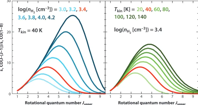
usually use the non-local thermodynamic equilibrium (non-LTE) radiative transfer calculations to model the observed CO spectral line energy distributions (SLEDs). Such models take the advantages of a large velocity gradient (LVG, e.g.Goldreich & Kwan,1974;Scoville & Solomon,1974;Sobolev,1960) statistical equilibrium method. One of the most popular radiative transfer code of such kind isRADEXthat calculates the fluxes of atomic and molecular lines produced in homogeneous clouds (van der Tak et al.,2007). From such models, the physical conditions of the molecular gas, such as gas density, gas temperature and the column density of the gas tracer, can be derived. Fig.1.11shows examples of different CO SLEDs generated by different conditions of the molecular gas.

30 20 10 0 1 2 3 4 5 6 7 8 9 sν C O( J– [J–1])/s ν C O(1 – 0)

Rotational quantum number Jupper

1 2 3 4 5 6 7 8 9

Rotational quantum number Jupper

log(nH

2

[cm

–3

_{]) =}

_3.0

_,

_3.2

_,

_3.4

_,

3.6 ,

3.8 ,

4.0 ,

4.2 Tkin

= 40 K

Tkin

[K] =

20 ,

40 ,

60 ,

80 ,

100 ,

120,

140 log(nH

2

[cm

–3

_{]) = 3.4}

Fig. 1.11 Figure adapted fromCarilli & Walter(2013) showing the CO SLEDs derived from different physical conditions shown in the legends. Left: The CO SLEDs based on a fixed gas temperature of 40 K and a varying gas density from 103.0cm−3to 104.2cm−3. Right: The CO SLEDs based on a fixed gas density of 103.4cm−3and a varying gas temperature from 20 K to 140 K.

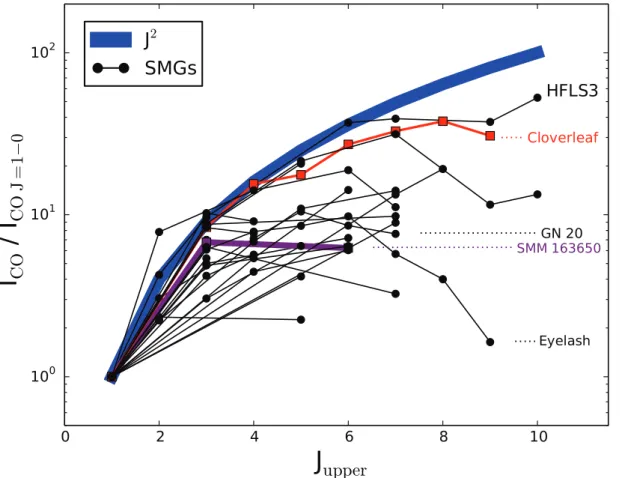
The CO SLED for high-z SMGs shows a variety of shapes, with the peak mostly located above Jup≳4 as

shown in Fig.1.12, with thermalised level populations being up to Jup∼ 6. Comparing to the CO SLED of

the SMGs, those of the local starbursts (M 82 and NGC 253) show much weaker excitation. This indicates that the excitation conditions in SMGs are quite extreme. Nevertheless, the CO SLEDs of local ULIRGs also share similarities with those of the SMGs. For the most striking case of HFLS 3 (Riechers et al.,2013), the CO SLED is even comparable to that of the lensed QSO Cloverleaf (Solomon et al.,2003).

Thermal collisional excitation is commonly seen in the ISM, but there are also other excitation mecha-nisms that influence the molecular line emission/absorption, especially in the extreme ISM environments

(27)

14 Introduction

like SMGs. Shocks2can be a significant way to excite the molecular gas as found in NGC 6240 through analysis of the CO SLEDs (Meijerink et al.,2013). Strong radiation from active galactic nuclei (AGN) can also excite CO SLEDs, and the signature is usually seen in very high excitation levels (Jup≳10) of the CO

lines. Such a signature usually presents a rather flat CO SLED at the high-J end, being different from the SLED generated from other excitation mechanisms.van der Werf et al.(2010) show a good example of a local AGN-dominated ULIRG, Mrk 231, where the Jup≳10 part of the CO SLED is dominated by and X-ray

dominated region related to the central AGN. As mentioned in Section1.2.1, gas tracers, such as the submm H2O lines, can be dominated by far-IR pumping, especially for the Eup≳200 K lines (e.g.González-Alfonso et al.,2014,2010;Omont et al.,2013;Yang et al.,2013,2016). Because the excitation of the H2O lines comes

from both collisional (dominating the lines with Eup≲150 K), and also from far-IR, the H2O SLED will thus

help us to understand not only the physical properties of the molecular gas but also the far-IR radiation field, namely the properties of dust emission. Thus, the H2O lines become a unique probe for studying the

ISM in high-z SMGs.

Fig. 1.12 Figure adapted fromNarayanan & Krumholz(2014) showing the CO SLEDs from different SMGs as indicated by the black dots. Red data points show the lensed QSO, Cloverleaf, while the violet line shows SMM 163650. The blue stripe shows the Rayleigh–Jeans limit assuming local thermodynamic equilibrium (LTE). SeeNarayanan & Krumholz(2014) for references.

2_{Shock wave is defined by a pressure-driven disturbance propagating faster than the sound velocity. In such cases, the}

upstream material cannot dynamically respond to the upcoming material, resulting in an irreversible change. The two main types of shocks happen in the gas phase ISM are J-shock and C-shock. For the former, the properties of the ISM appear as a jump from the preshock front to the postshock front. While for the latter, the shock front is much thicker than the cooling length scale, the jump condition is no longer available.

(28)

1.2.3 Important chemical processes revealed by the molecular lines

Chemistry is another important prospective for the ISM, that describes the formation, destruction and excitation of molecules in astronomical environments. The subject not only includes the chemical aspects of molecules, but also influences the diagnostics of the physical conditions, since the chemical reactions, especially those happening in the gas-phase ISM, are closely related to the radiation field and/or the ionization states.

Fig. 1.13 The formation routes and related chemical reactions of H2O molecules as described in the text.

Figure adapted fromvan Dishoeck et al.(2013).

Take H2O for example, as shown in Fig.1.13, H2O can be formed through both solid-state and

gas-phase chemical reactions (van Dishoeck et al.,2013). On dust-grain mantles (shown in blue colour in the figure), surface chemistry dominates the formation of H2O molecules. Then they can be released into the

gas phase ISM through sublimation. While in the gas phase, H2O can be produced through two routes:

the neutral-neutral reaction (shown in red colour in the figure), usually related to shocks, creates H2O

via O + H2−−→ OH + H; OH + H2−−→ H2O + H at high gas temperature. At lower gas temperature, the

ion-neutral reactions (shown in green colour) in photon-dominated regions (PDRs), cosmic-ray-dominated regions and X-ray-dominated regions (e.g.Meijerink & Spaans,2005) generate H2O from O, H+, H+₃ and

H2, with intermediates such as O+, OH+, H2O+and H3O+, and finally H₃O++ e −−→ H₂O + H. Thus, the

H2O+lines can be among the most direct tracers of the cosmic-ray or/and X-ray ionization rate (e.g.Gérin et al.,2010;González-Alfonso et al.,2013;Neufeld et al.,2010) of the ISM. Recent detections of H2O+lines

in extragalactic environments (van der Tak et al.,2016;Yang et al.,2016) show rich information about the dominating chemical process and also the ionisation states.

(29)

16 Introduction

1.3 Studying the SMGs through the cosmic telescope: gravitational lensing

1.3.1 Basic principles of gravitational lensing

The physical phenomenon called gravitational lensing was first raised byEinstein(1936), showing that the travelling path of the photons from distant objects can be perturbed by the inhomogeneously distributed matter along their trajectories, being much like photons passing through lenses, but from the effect of gravity (gravitational lensing). In the real cases, such an effect is usually minor, and it slightly distorts the appearance of the source. This mild effect is called weak gravitational lensing (e.g.Bartelmann & Schneider,2001). In rare cases, the foreground gravity potential (usually formed by massive galaxies or galaxy clusters) is strong enough to produce multiple images, arcs, or even Einstein rings (see Fig.1.14for an illustration). This is called strong gravitational lensing. We will briefly describe some basic principles of lensing in the following paragraphs.

a bb c d

a c d

Fig. 1.14 Figure adapted fromTreu(2010) (image courtesy of P. Marshall) displaying an optical analogy of the gravitational lensing phenomenon. The optical properties stem of a wineglass share similarities with the galaxy-type deflectors. The analogies are: a) viewing a distant object directly; b) multiple images in observed in the image plane; c) an Einstein ring; d) two arcs in the image plane. The corresponding astrophysical real images (Moustakas et al.,2007) are also shown in the lower left corner of each insets.

A typical gravitational lens system is shown in Fig.1.15. The mass over-density (deflector) resides at redshift zd, corresponding to an angular diameter distance of Dd. The background lensed object

emits photons at redshift zs, corresponding to a distance of Ds. The distance between the source and

the deflector is Dds(note that because the distance is not additive, Dds̸= Ds− Dd). After defining the

observation axis indicated by the dashed line in the figure, we find two planes perpendicular to our observation axis: the source plane where the background source emission can be described and the lens plane that characterises the mass distribution of the deflector. Then, we can write the position of a source at the angular position ⃗β as⃗η = ⃗βDs. The deflection angle is ⃗ˆα while the angle of the source in the image

plane is ⃗θ. Due to the deflection of the light emitted by the background object, the observer receives the light coming from the source from ⃗β as if it was emitted at the angular position ⃗θ (corresponding to an impact parameter ⃗ξ =⃗θDd). If ⃗ˆα, ⃗β and ⃗θ are small, we can describe the relation of these three angles using

the angular diameter distance as,

⃗θDs= ⃗βDs+ ⃗ˆαDds. (1.11)

By defining the angular diameter distance between the deflector and source as⃗α(⃗θ) = (Dds/Ds)⃗ˆα(⃗θ), we

can further rewrite Eq.1.11into

⃗β =⃗θ −⃗α(⃗θ), (1.12)

which is usually called lens equation. When this equation has multiple solutions corresponding to multiple images, strong lensing occurs. The most common configurations of such kind of strong lensing are shown

(30)

1.3 Studying the SMGs through the cosmic telescope: gravitational lensing 17

in Fig.1.14. In such systems, the strong-lensing cross section is defined by the solid angle in the source plane that produces multiple images. If we defineψ as the two-dimensional lensing potential, the Jacobian of the transformation from image to the source plane can be written as

A =∂⃗β ∂⃗θ= δi j− ∂2_ψ ∂⃗θi∂⃗θj = Ã 1 − κ − γ1 −γ2 −γ2 1 − κ + γ1 ! = (1 − κ) Ã 1 0 0 1 ! − γ Ã cos 2φ sin 2φ sin 2φ −cos2φ ! , (1.13)

whereκ describe the convergence of the image (Fig.1.14), which is also called dimensionless surface mass density κ(⃗θ) ≡Σ(Dd⃗θ) Σcr with Σcr= c2 4πG Ds DdDds , (1.14)

where is the critical surface mass density that defines the chacteristic scale for the occurrence of strong lens-ing features likes arcs and multiple images. Whileγ describes the shear, which has two shear components

γ1andγ2that γ ≡ γ1+ iγ2= ¯ ¯γ¯¯e2iφ, (1.15) which have Ãγ1 γ2 γ2 γ1 ! = γ Ã cos 2φ sin2φ sin 2φ cos2φ ! . (1.16) G ra vi ta tiona l L ens ing Convergence + shear Source Image Convergence alone

Fig. 1.15 Left: Figure adapted fromBartelmann & Schneider(2001) displaying a sketch of a typical gravita-tional lensing system (see text for descriptions). Right: Sketch showing the effect of convergence and shear adapted fromUmetsu(2010).

(31)

18 Introduction

The inverse of the determinant of the Jacobian matrix gives the magnification, as

µ = 1 detA = 1 (1 − κ)2₋¯ ¯γ¯¯ 2 (1.17)

In the cases of extended sources, the magnification also depends on the distribution of the surface brightness of the background source. The magnificationµ reflects the increase of total emission area, corresponding to the total amplification of its integrated flux.

In Eq.1.17, the locations (satisfying 1 − κ = ±γ) for which detA = 0 have infinite magnification. The corresponding source plane positions are the caustics, while these locations are called critical curves in the image plane. However, in the real astronomical practice, the finite object size keeps its observed magnification finite, which is usually a few up to more than one hundred for a typical galaxy-galaxy lensing system (e.g.Meylan et al.,2006).

Strong gravitational lensing is a powerful tool for not only studying the mass structure of the foreground deflector, the geometry of the Universe, but also offering precious opportunities to observe the weak background source, by magnifying its flux by up to more than an order of magnitude, and its size by a smaller factor. This offers a cosmic telescope that helps us to detect emission from the background source that is beyond our observation limits. It can also help us to understand the mass structure of the foreground source and to test models of the Universe’s geometry. Our work thus takes advantage of strong gravitational lensing to focus on the emission from the background source, by first searching for a sample of lensed candidates using large survey data and then performing follow-up observations of the molecular gas and dust in the SMGs. The related description of the survey and the source selection are given in Sections2.1and2.2.

1.3.2 Studies of the high-redshifted strongly-lensed SMGs

Although strong gravitational lensing offers a powerful tool for studying the high-redshift universe, the surface density of such kind of sources is very low. Depending on the observation depth, current telescopes can usually achieve detection of strong lensing at a rate of ∼ 1 out of 1000 galaxies (Marshall et al.,2005). The observations of the ISM of such strongly lensed galaxies at high-redshift therefore limited, and usually in those brightest systems. Such systems include the famous gravitationally lensed quasar/AGN-dominated sources, Cloverleaf (e.g.Barvainis et al.,1994;Bradford et al.,2009;Weiß et al.,2003), APM 08279+5455 (e.g.

Downes et al.,1999;Lewis et al.,1998;Riechers et al.,2009;Weiß et al.,2007) and IRAS F10214+4724 (e.g.

Broadhurst & Lehar,1995;Downes et al.,1992;Rowan-Robinson et al.,1991).

A detailed study of a lensed submm bright galaxy at z = 2.8, SMM 02399-0136, was presented by

Ivison et al.(1998).Frayer et al.(1998) report the CO detection in a z = 2.8 submm-selected bright galaxy SMM 02399-0136, with an SFR ∼ 103M_⊙. Later, the same team has discovered another similar galaxy, SMM J14011+0252, having a similar total molecular gas mass and SFR (Frayer et al.,1999). All the three sources were selected in a submm survey using SCUBA through lensing clusters (Smail et al.,1998). The massive molecular gas reservoirs indicate the link of these galaxies to the present day massive elliptical galaxies. One of the most remarkable cases of the strongly lensed sources discovered in the field of such massive galaxy clusters is SMM J2135-0102 (Swinbank et al.,2010). The z = 2.3 source has been magnified by a factor of 32, which offers a unique opportunity for a detailed study of the physical properties of the source. The source thus has been observed intensively using the ground-based telescopes like GBT, NOEMA, APEX, and SMA (Danielson et al.,2011). Fig.1.16shows the observed spectra of the CO, [CI], and

(32)

1.3 Studying the SMGs through the cosmic telescope: gravitational lensing 19

HCN lines. By analysing the CO line excitation of the source,Danielson et al.(2011) show that the source share similarity in the CO excitation condition as in local starburst galaxies. The CO ladder includes at least two phases with different gas densities and temperatures. Combing the lensing magnification, the work shows that the Kennicutt–Schmidt relation breaks down on scales of < 100 pc.

Fig. 1.16 Figure adapted fromDanielson et al.(2011) showing the CO, [CI], and HCN line spectral of the

source SMM J2135-0102 by GBT, NOEMA, APEX, and SMA.

With the development of efficient selecting the strongly lensed candidates using large area submm surveys (Negrello et al. 2010,2007, as described in Section2.1), a large number of lensed candidates were identified. This technique offers new opportunity to study the submm-bright sources, usually with an intrinsic surface SFR around several hundred M⊙yr−1kpc−2.

One of the examples of such studies include the lensed source discovered by the Herschel Astrophysical Terahertz Large Area Survey (H-ATLAS,Eales et al.,2010), H-ATLAS J114637.9-001132 (Fu et al. 2012, see also other examples by e.g.Conley et al. 2011;Cox et al. 2011;Gavazzi et al. 2011). Through high-resolution observations of the dust continuum using SMA, KECK K-band imaging and JVLA observation of the CO(1–0) tracing the total molecular gas, the work reveals that the system is a gas-rich starburst galaxy similar local ULIRGs and other unlensed SMGs. The total molecular gas mass contributes ∼ 68% visible baryonic mass. There is also a ∼ 4 kpc separation between the spatial location of the stellar component and that of the dust and molecular gas. Such an offset has also been found in other high-redshift lensed SMGs (e.g.Dye et al.,2015).

The most stunning example is shown by the high-resolution ALMA images of the source SDP 81 (H-ATLAS J090311.6+003906) as further described in Chapter5. With the help of boosted brightness and spatial resolution, these images allow us to study the high-redshift galaxy in unprecedented detail.

(33)

20 Introduction

1.4 Thesis outline

In this thesis, I will present a series of works focused on the molecular gas, from the observational perspectives, in a sample of strongly gravitationally lensed SMGs. By studying mostly H2O and CO lines,

we learn the physical conditions of the star-forming molecular gas content and also the thermal dust emission properties. Through the analysis of these properties, we have gained a better view of the star formation conditions/processes within these SMGs.

In Chapter2, I will briefly describe our sample selection. Then I will present the work on H2O line

observations in the SMGs in Chapter3. Chapter4shows our multiple-J CO and [CI] line observations,

from which we study the properties of the bulk of molecular gas properties. The high angular-resolution study of two SMGs via ALMA and NOEMA extended configurations is presented in Chapter5. In the end, the thesis work is summarised in Chapter6together with prospectives.

(34)

Chapter 2 Source selection

You behold Atlas supporting the whole of heaven.

Propertius, Elegies

2.1 Identifying the strongly lensed candidates

The key to study the SMGs through strong gravitational lensing is to find an efficient way to identify such systems from large survey data. However, the strong gravitational lensing at submm bands is rare (less than

Efficiently choosing the lensed sources

Fig. 2.1 The 500µm number counts of different types of galaxies. The solid violet line shows the number counts from radio active galactic nuclei (blazars), while the green one shows that of nearby late-type galaxies. Solid red line shows the number counts of SMGs without lensing, while the dashed red line show the results considering the lensing. The black curve shows the total number counts predicted while the observation data points are derived from the H-ATLAS maps. The yellow square shows the region from where lensed candidates can be most efficiently selected. (Figure adapted fromNegrello et al. 2010).

Physical conditions of the interstellar medium in high-redshift submillimetre bright galaxies

HAL Id: tel-01661478

https://tel.archives-ouvertes.fr/tel-01661478

Physical conditions of the interstellar medium in

high-redshift submillimetre bright galaxies

Chentao Yang

To cite this version:

Physical conditions of the

interstellar medium in high-redshift

submillimetre bright galaxies

Thèse de doctorat de University of the Chinese Academy of Sciences

et de l'Université Paris-Saclay, préparée à l’Université Paris-Sud

École doctorale n°127 Astronomie et Astrophysique d’Île-de-France :

Institut d'Astrophysique Spatiale (IAS),

Purple Mountain Observatory (PMO)

Chentao YANG

NNT

:

2

0

1

7

SAC

L

S3

6

1

Acknowledgements

Résumé

Table of contents

Chapter 1

Introduction

1.1 Discoveries of the submillimetre-bright galaxies at high-redshift

Template:

Arp

220

1.2 Studying the high-redshift SMGs with various molecular gas tracers

Trace Gas

Trace

Radiation

A

B

E

E

B

hν

ALMA

NOEMA

log(nH

[cm

]) =

3.0

,

3.2

,

3.4

,

3.6

,

3.8

,

4.0

,

4.2

Tkin

= 40 K

Tkin

[K] =

20

,

40

,

60

,

80

,

100

,

120,

140

_{]) =}

_3.0

_,

_3.2

_,

_3.4

_,

_{]) = 3.4}