HAL Id: insu-01285088
https://hal-insu.archives-ouvertes.fr/insu-01285088
Submitted on 8 Mar 2016
HAL is a multi-disciplinary open access
archive for the deposit and dissemination of
sci-entific research documents, whether they are
pub-lished or not. The documents may come from
teaching and research institutions in France or
abroad, or from public or private research centers.
L’archive ouverte pluridisciplinaire HAL, est
destinée au dépôt et à la diffusion de documents
scientifiques de niveau recherche, publiés ou non,
émanant des établissements d’enseignement et de
recherche français ou étrangers, des laboratoires
publics ou privés.
Martian Temperature Profiles Measured by MAVEN
and MRO from 20 to 160 km
Hannes Gröller, Roger V. Yelle, Tommi T. Koskinen, Franck Montmessin,
Gaetan Lacombe, David Kass, Armin Kleinböhl, T. Schofield, D. J. Mccleese,
Nick Schneider, et al.
To cite this version:
Hannes Gröller, Roger V. Yelle, Tommi T. Koskinen, Franck Montmessin, Gaetan Lacombe, et al..
Martian Temperature Profiles Measured by MAVEN and MRO from 20 to 160 km. 47th Lunar and
Planetary Science Conference, Mar 2016, The Woodlands, Texas, United States. pp.1811.
�insu-01285088�
MARTIAN TEMPERATURE PROFILES MEASURED BY MAVEN AND MRO FROM 20 TO 160 KM.
H. Gröller1, R. V. Yelle1, T. T. Koskinen1, F. Montmessin2, G. Lacombe2, D. Kass3, A. Kleinböhl3, T. Schofield3, D. McCleese3, N. M. Schneider4, J. Deighan4, S. K. Jain4, and B. M. Jakosky4
1Lunar and Planetary Laboratory, University of Arizona, Tucson, AZ, USA, 2LATMOS, Université Versailles
Saint-Quentin / CNRS, Guyancourt, France, 3Jet Propulsion Laboratory, California Institute of Technology, Pasadena, CA, USA, 4Laboratory for Atmospheric and Space Physics, University of Colorado, Boulder, CO, USA.
Email: hgr@lpl.arizona.edu
Introduction: We combined the temperature
profile retrieved from the Imaging UltraViolet Spectrometer (IUVS) on Mars Atmosphere and Volatile EvolutioN (MAVEN) [1] and from the Mars Climate Sounder (MCS) on Mars Reconnaissance Orbiter (MRO) [2] to obtain a measured temperature profiles spanning the altitude range from the lower (~20 km) up to the upper (~160 km) atmosphere. A temperature profile that covers such a large altitude range will allow us to investigate coupling among atmospheric regions both for static structures controlled by radiative exchange and for propagating structures such as tides and waves.
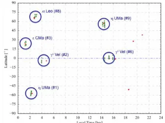
To construct the merged temperature profile we required IUVS and MCS measurements at similar locations (latitude, longitude, and local time). The latitude and local time distribution of the measurements is shown in Figure 1.
Figure 1: Latitude and local time distribution of stellar
occultations from IUVS (red dots) and observations executed by MCS (green dots). The blue circles indicate which stellar occultations and observations are combined for the temperature profile and which star was targeted during the IUVS stellar occultations.
Instruments and Data Processing: The upper
atmosphere (roughly between 90 and 160 km) is probed by the IUVS instrument using the FUV channel and the lower atmosphere (from the surface up to 90 km) is measured by the MCS instrument. The FUV
channel of the IUVS instrument covers the wavelength range from 110 nm up to 190 nm.
IUVS Instrument. UV stellar occultations have
proved to be a powerful technique to study the structure and composition of the upper atmosphere.
The measured transmission spectrum is fitted at each altitude using the Levenberg-Marquardt algorithm to retrieve the best-fit column densities assuming absorption by CO2 and O2. These obtained slant
column density profiles are inverted to get the corresponding local number densities by using the Tikhonov regularization method [3].
The temperature profile is calculated by applying the hydrostatic equilibrium constraint to the local CO2
number densities [4]. A detailed description of the whole retrieval procedure to get temperature profiles from IVUS stellar occultations can be found in [5,6,7].
MCS Instrument. MCS is a 9 channel visible and
IR radiometer optimized for atmospheric limb (horizon) sounding [8]. In addition to the bolometric visible channel, there are 8 IR channels spanning 12 µm to 42 µm. Each channel is composed of an array of 21 detectors that are pointed at the limb providing a radiance profile from the surface to ~80 km with a vertical resolution of ~5 km.
MCS obtains daily global (pole-to-pole) coverage at two primary local times (3 am/3 pm). For these observations, MCS also acquires on-planet views to help sound the lowest 1-2 scale heights in high opacity conditions. MCS can use azimuth articulation to observe additional local times [9] and to target specific locations (such as the IUVS stellar occultations) within the MCS latitude/local time observation envelope.
The radiance profiles are inverted via a Chahine method [10] to retrieve vertical profiles of temperature, dust and water ice extinction versus pressure. This is an iterative technique that simultaneously solves for all fields by minimizing the radiance residuals [11, 12].
Results: By combining temperature profiles from
the IUVS and the MCS instruments we get a profile that ranges from around 20 km up to almost 160 km. Figure 2 shows as an example of the combined temperature profiles for a latitude of ~5° S and a local time of ~4.5 hrs but for different longitudes. The longitudes of the temperature profiles are at ~177° W,
1811.pdf 47th Lunar and Planetary Science Conference (2016)
~50° E, and ~9° W and colored in red, green, and blue, respectively. In addition to the temperature profiles the CO2 saturation temperature is plotted as a dash-dotted
black line.
Despite the gap between the two temperature profiles at around 90 km, one can see that the temperature transition connects the two datasets very well. Also the wave structures of the MCS profiles seem to propagate from the lower altitudes up to the upper altitudes of the IUVS profiles.
Figure 2: Temperature profiles for the upper and lower
atmosphere from the IVUS (solid) and MCS (dash), respectively. The profiles are for a latitude of ~5° S and a local time of ~4.5 hrs but for different longitudes. The longitudes of the temperature profiles are at ~177° W, ~50° E, and ~9° W and colored in red, green, and blue, respectively. The black dash-dotted line illustrates the CO2
saturation temperature.
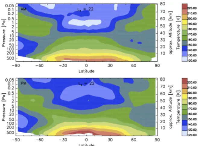
Global and Regional Context: In addition to the
profiles co-located with the stellar occultations, MCS provides the global and regional context for the lower and middle atmosphere. This places the targeted observations in the overall seasonal context delineates the global circulation in the lower and middle atmosphere (Figure 3). The global and regional coverage from MCS will allow for the identification of the waves and/or tides that propagate vertically from the middle atmosphere into the upper atmosphere as well as those that do not propagate [13, 14].
Future Plans: The IUVS instrument is designed to
simultaneously record stellar occultations in two channels, the FUV channel and the MUV channel. The FUV channel ranges from 110 nm up to 190 nm and the MUV channel from 180 nm up to around 330 nm. When using the combined FUV and MUV transmission spectrum for the retrieval a temperature profile from roughly 160 km down to 30 km can be
obtained and thus also temperatures in the gap region between IUVS (FUV) and MCS may be available. Eventually we will be able to combine both FUV and the MUV transmission spectrum with MCS limb profiles to determine a temperature profile from the near surface to the upper thermosphere.
Figure 3: Zonal mean lower and middle atmosphere
temperature cross-sections from MCS at the same season as the observations in figure 1. These are in a 2° Ls bin at 3 am and 3 pm and show the expected configuration for early northern spring (Ls 22°) with a fairly symmetric circulation, although the northern vortex is already weakening signficatnly.
References: [1] Jakosky, B. M. et al. (2015) Space
Sci. Rev., 195, 3–48, doi:10.1007/s11214-015-0139-x.
[2]Zurek and Smrekar (2007) JGR, 112, E05S01, doi: 10.1029/2006JE002701. [3] Quémerais, E. et al. (2006) J. Geophys. Res., 111, E09S04, doi:10.1029/2005JE002604. [4] Snowden D. et al. (2013) Icarus, 226, 552–582. [5] Montmessin, F. et al. (2006) J. Geophys. Res., 111, E09S09, doi:10.1029/2005JE002662. [6] Gröller H. et al. (2015) Geophys. Res. Lett., 42, 9064–9070, doi:10.1002/2015GL065294. [7] Sandel B. R. et al. (2015) Icarus, 252, 154–160. [8] McCleese et al. (2007), JGR, 112, E05S06 doi: 10.1029/2006JE002790. [9] Kleinböhl et al. (2013),
Geophys. Res. Lett. 40, 1952-1959, doi: 10.1002/grl.50497. [10] Chahine (1972), J. Atmos.
Sci., 29. [11] Kleinböhl et al. (2009), JGR 114,
E10006, doi: 10.1029/2009JE003358. [12] Kleinböhl
et al. (2011), JQRST, 112, 1568-1580. [13] Lee et al.
(2009), J. Geophys. Res. 114, E03005, doi: 10.1029/2008JE003285. [14] Guzewich et al. (2012) J.
Geophys. Res. 117, E03010, doi: 10.1029/2011JE003924.
1811.pdf 47th Lunar and Planetary Science Conference (2016)