Precision cosmology with the large-scale structure of the universe

(1)

HAL Id: tel-01235603

https://tel.archives-ouvertes.fr/tel-01235603

Submitted on 30 Nov 2015

HAL is a multi-disciplinary open access archive for the deposit and dissemination of sci-entific research documents, whether they are pub-lished or not. The documents may come from teaching and research institutions in France or

L’archive ouverte pluridisciplinaire HAL, est destinée au dépôt et à la diffusion de documents scientifiques de niveau recherche, publiés ou non, émanant des établissements d’enseignement et de recherche français ou étrangers, des laboratoires

Precision cosmology with the large-scale structure of the

universe

Hélène Dupuy

To cite this version:

Hélène Dupuy. Precision cosmology with the large-scale structure of the universe. Cosmology and Extra-Galactic Astrophysics [astro-ph.CO]. Université Pierre et Marie Curie - Paris VI, 2015. English. �NNT : 2015PA066245�. �tel-01235603�

(2)

Universit´e Pierre et Marie Curie

Sorbonne Universit´es

´

Ecole doctorale de Physique en ˆIle-de-France Institut d’Astrophysique de Paris (IAP)

et

Institut de Physique Théorique (IPhT) du Commissariat à l’ Énergie Atomique et aux Énergies Alternatives (CEA) de Saclay

Precision cosmology with the

large-scale structure of the universe

par H´el`ene Dupuy

Th`ese de doctorat en cosmologie

dirig´ee par Francis Bernardeau (chercheur CEA, directeur de l’IAP)

pr´esent´ee et soutenue publiquement le 11/09/2015

devant un jury compos´e de (par ordre alphab´etique) :

Dr. Francis Bernardeau IAP, CEA Examinateur

Dr. Diego Blas CERN (TH-Division) Examinateur

Pr. Michael Joyce LPNHE Examinateur

Pr. Eiichiro Komatsu Max-Planck-Institut f¨ur Astrophysik

Rapporteur

Pr. Julien Lesgourgues RWTH Aachen University Rapporteur

(3)

6.1 Generalized definitions of displacement fields in the eikonal approxi-mation . . . 168 6.2 Impact on the nonlinear growth of structure . . . 170 6.2.1 Qualitative description . . . 170 6.2.2 Quantitative results in the case of streams of massive neutrinos172 6.3 Article “On the importance of nonlinear couplings in large-scale

neu-trino streams” . . . 174

Conclusions and perspectives 188

Acknowledgments 193

Remerciements 195

Résumé de la thèse en fran¸cais 218

(6)

Introduction

The title of my PhD thesis, “Precision cosmology with the large-scale structure of the universe”, encompasses a wide range of searches, all equally exciting. Cosmology is an ancient questioning: understanding what the universe is made of, how it formed, how it evolved since then and what its future is. Yet it is entering a new era, whence the denomination precision cosmology. The investigation method is still the same, i.e. switching back and forth between observations of the sky and formulation of theories, but lately the level of description has amazingly evolved.

The twentieth century has been a golden period for cosmology. On the theo-retical side, about a hundred years ago, Albert Einstein’s general relativity ([64]) brought the mathematical tools allowing to represent appropriately time and space in a gravitation theory. Soon after appeared the first models based on this theory to describe the structure of the universe and its time evolution. The expansion of the universe has been discovered at the same epoch, jointly thanks to the ob-servations of the astrophysicist Edwin Hubble (carried out and discussed between 1925 and 1929, [94]) and to the relativistic calculations of several theorists, such as Georges Lemaˆıtre (in 1927, [103]), Alexandre Friedmann (in 1922, [79]) and Willem de Sitter (in 1917, [53]). A cosmological model naturally emerged from the study of the physics at play in an expanding universe. It is the Big Bang theory, accord-ing to which the universe was born 13.8 billion of years ago (from a process called Big Bang and involving unimaginably high energies) and then progressively cooled down and dilated.

In this context, cooling down means dropping from a temperature1 _T _{⇠ 10}19

GeV to T ⇡ 2.73 K. Such di↵erent temperatures lead perforce to extremely di-1_{In cosmology, it is common to use the electronvolt as unit of temperature, or more precisely the}

electronvolt divided by the Boltzmann constant since 1 eV / kB⇡ 11604.5 K, kBbeing the

Boltz-mann constant (kB = 1.3806488⇥ 10 23 m2.kg.s 2.K 1). In practice, one omits the Boltzmann

constant so that T (K)⇡ 11604.5 T (eV).

(7)

versified physical processes. The chain of cosmological eras, each characterized by specific physical processes, is called thermal history of the universe. All stages of the thermal history are not equally understood. In particular, understanding mech-anisms involving energies that are not accessible in laboratories is very challenging. Some epochs are thus described very speculatively. Conversely, the Big Bang nu-cleosynthesis and the recombination era are particularly well depicted. The former is the process during which nuclei heavier than the lightest isotope of hydrogen are created thanks to the trapping of protons and neutrons that previously freely evolved in the cosmic plasma (T _{⇠ 1 MeV). The latter refers to the epoch at which} electrons and protons first became bound to form electrically neutral hydrogen atoms (T ⇠ 3000 K).

One specificity of the Big Bang model is that it predicts the existence of a radiation which started to propagate freely about 380 000 years after the Big Bang. This “cosmic microwave background”, detected incidentally in 1964 by the two physicists Arno Penzias and Robert Wilson ([128]), is nothing but the photons that emerged when the temperature of the cosmic plasma became lower than the temperature of ionization of hydrogen. Its detection was such a strong argument in favor of the Big Bang model that this discovery has been awarded the Nobel Prize in 1978. Nowadays, observing and studying carefully the cosmic microwave background is still one of the driving force of cosmology.

So far, the Big Bang model has not been ruled out by observations. Rather, each new set of cosmological data provided by exploration of space strengthens the so-called “standard model of cosmology”. This model relies on the Big Bang theory and assumes the existence of a cosmological constant, which mimics the acceleration of the expansion of the universe, and of cold dark matter, a form of matter proposed in response to some unexpected observations.

More precisely, two observational projects realized in 1998 by the scientific teams headed by the cosmologists Saul Perlmutter, Brian P. Schmidt and Adam Riess showed independently that the expansion of the universe is accelerating ([129,148]). This breakthrough has been honored with the Nobel Prize in 2011. Gravity being an attractive unstoppable force, astrophysicists originally thought that expansion could only decelerate. It has therefore been necessary to imagine a form of re-pulsive energy, capable of accelerating the expansion of the universe. This cosmic component of unknown nature has been called dark energy. In the standard model, it is characterized by a parameter denominated cosmological constant and

(8)

senting about 70% of the energy content of the universe. Note nevertheless that several alternatives to the cosmological constant (and thus alternatives to the stan-dard model) can be imagined to describe the same e↵ect. At this time, it is still very difficult to determine which representation of dark energy is the most credible. Hopefully, the Euclid space mission ([157]), proposed in 2005 to the European Space Agency and whose launch is planned for 2020, will enrich (or even conclude) the debate.

Besides, many observations suggest the presence of an unfamiliar form of matter, invisible and with a non-zero mass, called dark matter. Dark matter would explain for instance why galaxies and clusters of galaxies seem much more massive when one studies their gravitational properties than when one infers their mass from the light they emit or why the cosmic microwave background displays spatial fluctuations too faint to initiate the formation of structures by gravitational instability (see more details about gravitational instability in section 1.1). In the standard model of cosmology, this dark matter is assumed to be cold, i.e. made of particles whose velocity is already much smaller than the speed of light in vacuum when it decouples from other species. Unveiling the nature and the properties of those dark elements is a major challenge, at the core of modern cosmology. It is the main raison d’ˆetre of the Euclid mission.

Another very puzzling piece of modern cosmology is cosmic inflation. It is an idea that arose in the late seventies-early eighties to complement the Big Bang model (see the foundational works of the physicists Alexei Starobinsky ([172]), Alan Guth ([84]) and Andrei Linde ([110])). According to this theory, the primordial universe underwent an extremely fast and violent phase of expansion. Adding this step to the thermal history of the universe is useful in many ways to get a coherent whole. However, the paradigm of inflation is not yet perfectly controlled theoretically.

The agreement between the standard model of cosmology and observational surveys is remarkably good. So, at the present time, most cosmologists focus their e↵ort on the refinement of this model. The technical means available today allow to probe a huge quantity of astrophysical objects, of various nature, spread over very large areas of the sky. Specific developments, involving to a large extent numerical simulations and statistical physics, are necessary to deal with such an amount of data. But an exquisite exploration of the universe is useless if there is no comparable progress in theoretical cosmology.

The present thesis is a tiny illustration of the theoretical e↵orts currently

(9)

alized in order to anticipate a project such as the Euclid mission. As already mentioned, it has been designed primarily to examine the dark content of the uni-verse. It will moreover supply a catalog of galaxies of unprecedented richness and refinement, showing how galaxies and clusters of galaxies arranged with time to form tremendous filaments, commonly referred to as “the large-scale structure of the universe”.

The purpose of this thesis is twofold. A minor part of the time has been dedi-cated to a study designed to question a leading principle of cosmology, namely the cosmological principle. According to it, on very large scales2 (& 100 Mpc), the dis-tribution of matter in the universe is homogeneous and isotropic. Many predictions of modern cosmology ensue from it. In collaboration with Dr. Jean-Philippe Uzan and his PhD student Pierre Fleury, I have participated in a project consisting in simulating observations of supernovae in an inhomogeneous model of the universe in order to infer the impact of inhomogeneities on cosmology. We highlighted in particular the fact that using the same kind of geometrical models to interpret ob-servations corresponding to very di↵erent spatial scales could become inappropriate in the precision cosmology era (see chapter 1). The second topic I am specialized in is the enhancement of cosmological perturbation theory methods (see chapter 3 for a quick presentation of the current challenges of cosmological perturbation theory), especially within the nonlinear and/or relativistic regime(s). It is the main task developed in this thesis (see chapters 4, 5 and 6). In particular, I have proposed with my PhD advisor Dr. Francis Bernardeau a new analytic method, which is a multi-fluid approach, to study efficiently the nonlinear time evolution of non-cold species such as massive neutrinos (see chapter 2 for a modest overview of neutrino cosmology). This research project is at the interface between two topical subjects: neutrino cosmology and cosmological perturbation theory beyond the linear regime. The manuscript is organized as follows. In chapter 1, I take the example of an analytic questioning of the cosmological principle, in which I participated, to illustrate what is at stake in precision cosmology. Chapter 2 introduces basics of neutrino cosmology, with an emphasis on the key role it plays in the study of the formation of the large-scale structure of the universe. In chapter 3, I present standard results of cosmological perturbation theory on which I based most of my PhD work. The three next chapters expose the developments that I realized with my advisor with the aim of incorporating properly massive neutrinos, or any

non-2_{pc stands for parsec, defined so that 1 pc}

⇡ 3.1 ⇥ 1016_m. 7

(10)

cold species, in analytic models of the nonlinear growth of structure. Chapter 4 presents the method and questions its accuracy. Chapter 5 shows that the results presented in chapter 3, valid for cold dark matter, can then partly be extended to massive neutrinos. Finally, in chapter 6, I explain how our method can be helpful to determine the scales at which nonlinear e↵ects involving neutrinos are substantial and should be accounted for in models of structure formation.

(11)

Chapter 1 An illustration of what

precision cosmology means

1.1 Is the cosmological principle stringent enough for

precision cosmology?

A specificity of cosmology is that the system of interest is studied from inside. Furthermore, it is studied from a given position (the earth and surroundings) at a given time (epoch at which human beings are present on earth). Hence, since light propagates with a finite velocity and the universe has a finite age, only a portion of the universe can be reached observationally. This area is called observable universe and its boundary is called cosmological horizon. Consequently, cosmological models intended to describe the entire universe necessarily involve untestable assumptions (see e.g. [67] for discussions on this subject). In particular, as already mentioned, the standard model of cosmology relies on the cosmological principle, according to which the spatial distribution of matter is homogeneous and isotropic on large scales. This is encoded mathematically in the metric chosen to characterize the geometry of the universe, namely the Friedmann-Lemaˆıtre metric (see section 1.3.1).

Of course, the universe is not perfectly smooth. Otherwise, growth of structures from gravitational instability wouldn’t have been achievable. It is indeed commonly assumed that density contrasts existed in the primordial universe and initiated the formation of the large-scale structure. More precisely, this scenario is encapsulated in the inflationary paradigm. During this stage, in theory, quantum fluctuations of a cosmic scalar field became macroscopic, generating fluctuations of the metric

(12)

1.1. Is the cosmological principle stringent enough for precision cosmology?

([7,85,89,173,30,122]). Those metric fluctuations then resulted into density fluc-tuations, as predicted by general relativity, and thus into gravitational instability. The study of the time evolution of such fluctuations is generally performed thanks to cosmological perturbation theory (see chapter 3). In practice, this means adding perturbations, assumed to be small compared with the background quantities, in the Friedmann-Lemaˆıtre metric.

In its minimal version (in particular, in the absence of neutrinos), the standard model of cosmology allows to summarize the properties of the universe in six pa-rameters, called cosmological parameters. Defining them at this stage would be premature since none of the cosmological e↵ects behind them has been introduced yet. Nevertheless, for the record, here is the list:

• the primordial spectrum amplitude As,

• the primordial tilt ns,

• the baryon density !B,

• the total non-relativistic matter density !m,

• the cosmological constant density fraction ⌦⇤,

• the optical depth at reionization ⌧reion.

Their values are not predicted by the model, whence the importance of constraining them observationally. Several kinds of sources provide this opportunity. The lead-ing ones are Type Ia supernovae (SNIa), baryon acoustic oscillations (BAO) and the cosmic microwave background (CMB). A supernova is an astrophysical object resulting from the highly energetic explosion of a star. SNIa are particular super-novae whose spectra contain silicon but no hydrogen. They are useful in particular for the tracking of the expansion history of the universe. More precisely, they give information about the equation of state of dark energy (see e.g. [38, 146]). BAO are periodic fluctuations experimented by the baryonic1 components of the uni-verse and the knowledge of their properties brings also much to cosmology (see e.g. [5]). CMB observations provide an estimation of cosmological parameters with an exquisite precision, especially when combined with other astrophysical data ([137]). 1_{Baryonic means made of particles called baryons. In particular, all the matter made of atoms}

is baryonic.

(13)

1.1. Is the cosmological principle stringent enough for precision cosmology?

Since its first detection, the CMB has been inspected in great detail by several satellites looking for anisotropies in it. The motivation of such an investigation is the evidence of a dipole anisotropy2, presented in 1977 in [168] (which brought another Nobel Prize to cosmologists, this time George Fitzgerald Smoot and John C. Mather, in 2006). Higher order anisotropies3 _{have then been measured by the}

satellites COBE (launched in 1989, [167]), WMAP (launched in 2001, [10, 90]) and Planck (launched in 2009, [134]). Those space projects are complementary to ground-based experiments ([145,175,165]) and to balloon-borne instruments such as BOOMERanG4 (launched in late 1998, [52]) and Archeops (launched in 2002, [11]).

The combination “standard model of cosmology + perturbations” seems to be a satisfactory description. As proof, it is in agreement with most existing data. Such an accuracy is a bit surprising given the simplicity of the model and the thorough-ness with which the observable universe is explored. For instance, it is assumed that the matter is continuously distributed. This involves in particular a smooth-ing scale, not explicitly given in the model ([68]). Besides, some observables used in cosmology are “point sources” and thus probe scales at which the cosmological principle does not hold (and furthermore scales that are not accessible by numerical simulations, see section 1.2.2 for more details). This is particularly true for SNIa, which emit very narrow beams probing scales smaller than5 _{1 AU. For this reason,}

it has been argued in several references that the use of the cosmological principle might lead to misinterpretations (see for instance [33]). This is precisely the kind of questioning raised by the precision cosmology era.

2_{The earth is in motion in the universe. Consequently, when cosmologists measure the}

tem-perature of the CMB, one of the celestial hemispheres appears hotter than the other one. This phenomenon is called dipole anisotropy.

3_{Higher order anisotropies are reflective of plasma oscillations that develop when the last}

scat-tering surface is reached. They superimpose over dipole anisotropies.

4_{The BOOMERanG experiment has brought a strong support to the inflationary paradigm by}

showing that the geometry of the universe is Euclidean.

5_{AU stands for astronomical unit, defined so that 1 AU}

⇡ 1.5 ⇥ 1011_m.

(14)

1.2. Questioning the cosmological principle analytically

1.2 Questioning the cosmological principle analytically

1.2.1 Redshift, luminosity distance and Hubble diagram

Redshift

The universe being in expansion, one can observe that galaxies are moving away from the earth. This phenomenon is called recession of galaxies and is not due to a genuine proper motion of galaxies. Galaxies (and other astrophysical objects) are in fact taken away by the dilatation of the universe itself, even if some of them have a proper motion oriented towards us. Because of this relative displacement, the observed wavelengths obs are shifted to longer wavelengths (compared to the

emitted ones em). It is known as cosmological redshift, denoted z and defined so

that (see section 1.3.4 for a more general interpretation)

z = obs em

em

. (1.1)

More precisely, in his contribution to the discovery of the expansion of the universe, Edwin Hubble brought to light a law stating that the recession velocity6, vrec,

of galaxies is proportional to their distance7 d. Actually, this relation had been previously found by Georges Lemaˆıtre but remained almost unnoticed since stated in French. It reads

vrec = H0d, (1.2)

it is called Hubble’s law and H0 is Hubble’s constant. H0 is usually not considered

as part of the six cosmological parameters of the standard model of cosmology but it can be readily computed once those parameters are known8. Its value is currently estimated to be H0= (67.8± 0.9) km.s 1.Mpc 1([137]). To get information about

the expansion of the universe, it is thus useful to make measurements of velocities (or equivalently redshifts) on the one hand and of distances on the other hand.

6_{The recession velocity is the observed velocity to which the peculiar velocity has been}

sub-tracted.

7_{The distance at play in Hubble’s law is the distance between the source and the observer at}

the observation time. Because of expansion and since the speed of light is finite, this distance is larger than what it was at the emission time.

8_{Note nevertheless that, H}

0being in one-to-one correspondence with the standard cosmological

parameter ⌦⇤, H0 is sometimes considered as a cosmological parameter instead of ⌦⇤. In practice,

the nuance is inconsequential (provided that dark energy is assumed to be a cosmological constant).

(15)

Luminosity distance

Distances are not directly measurable. What observers can measure when they probe the sky is e.g. the angular diameter between two points or the amount of en-ergy collected by their telescopes. Cosmologists have introduced several definitions of distances from these observables. For instance, the “luminosity distance” of a source, DL, is easy to define with the help of the intrinsic luminosity of the source

Lsource (energy emitted per unit of time) and of the observed flux Fobs (energy

received per unit of time and surface). It is given by

Lsource= 4⇡D2LFobs. (1.3)

SNIa are extremely bright. Furthermore, after their apparition in the sky, the time evolution of their brightness is very well known, which allows one to calibrate their intrinsic luminosity. Those particularities make them precious suppliers of luminosity distances. Such sources are often called standard candles.

Hubble diagram

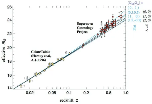
Building diagrams luminosity distance versus redshift is an efficient way of probing the history of the expansion of the universe since redshifts and distances are related via cosmological parameters. Such diagrams, naturally called Hubble diagrams, are largely used in modern cosmology (see e.g. [2]). An example is given in figure 1.1.

1.2.2 Misinterpretation of Hubble diagrams

The main message of [33] is that, to meet the requirements of precision cosmology, it is crucial to model accurately the propagation of the ultra-narrow beams produced by SNIa. Otherwise, using those observables as widely as it is done in cosmology would be inappropriate.

The fact that there seems to be a paradox between the real universe and its smooth representation was already discussed in the sixties ([199,50,19,83,98,144]). More recently, consequences regarding the interpretation of Hubble diagrams have been studied. In particular, according to general relativity, the presence of massive objects (such as clusters of galaxies) a↵ects the geometry of the universe. Since the way light propagates depends on the geometry, this results into a modification of the observed luminosity of sources. This phenomenon is called gravitational

(16)

Figure 1.1: One example of a Hubble diagram. It has been obtained from the observation of 42 high-redshift SNIa of the Supernova Cosmology Project and 18 low-redshift SNIa of the Cal`an/Tololo Supernova Survey. mB is the apparent

magnitude in the spectral band B, the magnitude m being related to Lsource via

m = 2.5 log Lsource+ 4.76. Authors: Perlmutter et al., [129].

lensing and it has been pointed out that it probably induces a scattering in Hubble diagrams ([99, 80, 191, 190, 192]). Because of the thinness of the beams emitted by SNIa, such beams spend most of their propagation time in underdense regions (and rarely, but sometimes, encounter clusters of matter). They are a priori too narrow for the e↵ects of such fluctuations of density to be negligible. Yet, Hubble diagrams are interpreted assuming that the geometry of the universe is on average homogeneous and isotropic.

Perturbative approaches, i.e. descriptions in which perturbations are added in the metric, have been proposed ([92, 39, 54]). However, in these works, there is still a smoothing scale at play. It is of the order of 1 arcminute9 _{whereas lensing}

dispersion arises to a large extent from subarcminute scales (see e.g. [48]). Besides, performing an average is problematic since SNIa probe the sky in directions where the density of matter encountered is smaller than the cosmological average (contrary

9_{The arcminute is a unit of angular measurement defined so that 1 = 60 arcminutes.} 14

(17)

to the beams of BAO and CMB, which are large enough for the average density encountered to be representative of the overall cosmological density, [195]). Hubble diagrams are thus prone to an observational selection e↵ect. All these problems are discussed in detail in [33].

Numerical simulations are an alternative to analytic modeling which can take inhomogeneities into account. However, it has been argued in [33] that, because of the limitation in resolution, only the distribution of matter encountered by beams larger than a few tens of kpc can be accurately described by N-body simulations. It is much wider than the characteristic diameter of a SNIa light beam.

1.2.3 An idea to test analytically the impact of inhomogeneities

Since a theoretical study seems necessary to investigate the way in which inhomo-geneities a↵ect the aspect of Hubble diagrams, we decided to elaborate analytically a toy model, representing a very inhomogeneous universe, and to study propaga-tion of light in it. More precisely, we chose to consider a geometry of the type “Swiss cheese”. Swiss-cheese configurations are obtained from a homogeneous and isotropic basis (i.e. a Friedmann-Lemaˆıtre metric) by removing spheres of matter at some places and replacing them by point masses, equal to the mass removed (see figure 1.2 for an illustration and [65,158] for the cornerstones of Swiss-cheese representations).

Figure 1.2: A Swiss-cheese configuration. The background is homogeneous. Spheres are empty except at their centers, where a point mass is present. The point mass is equal to the density of the background multiplied by the volume of the blank area surrounding it.

Our model is not intended to be realistic but rather to test the impact of inho-mogeneities on light propagation. From a theoretical point of view, it is as justified as the standard homogeneous and isotropic description because it is an exact solu-tion of general relativity which preserves the global dynamics (see secsolu-tion 1.3 for more details).

As a first step, we studied analytically the e↵ect of light crossing a single hole 15

(18)

1.3. Generalities about propagation of light in a Swiss-cheese model

and implemented it in a Mathematica program. It was then easy to predict the e↵ect of several holes. We proposed to do it with the help of Wronski matrices (see our paper, presented in section 1.5). Eventually, we simulated Hubble diagrams by imagining SNIa beams evolving in our Swiss-cheese universe. To do this, we took inspiration from the SNLS 3 data set ([38]).

The cosmological parameters of this mock universe being under control, we have been able to test the impact of inhomogeneities on cosmology (see section 1.4).

Note that using Swiss-cheese models to study the e↵ect of inhomogeneities is not new at all. The specificity of our study is that it is neither a “modern” Lemaˆıtre-Tolman-Bondi (LTB) solution, which is an extension of Swiss-cheese solutions in which point masses are replaced by continuous gradients of density (here is only a sample of the existing LTB studies: [31, 116,24, 185, 32, 35, 183,176, 74, 200, 72,73,143,151, 150,121,40,149,70]) nor a real step backwards into the original works on Swiss-cheese models ([98] and [62]) because our investigation is totally embedded in the framework of modern cosmology. Actually, we were interested in testing a discontinuous distribution of matter, which is not the case for LTB or perturbative approaches, in order to avoid the compensation e↵ects due to a finite smoothing scale. Consequently, we did not expect to obtain results similar to those of the literature.

1.3 Generalities about propagation of light in a

Swiss-cheese model

Rather than starting with general considerations about general relativity, I will merely introduce progressively the concepts that help to understand my PhD work. Comprehensive presentations of general relativity suited to the study of cosmology can be found in a broad collection of references (see in particular the indispensable [193] and [120]).

1.3.1 The homogeneous background

The standard model of cosmology assumes that gravitation is well described by gen-eral relativity. In gengen-eral relativity, time and space are not independent quantities, whence the use of the concept of spacetime. In standard cosmology, spacetimes encompass four dimensions and are mathematically characterized by a quantity

(19)

called metric. The Friedmann-Lemaˆıtre metric emerges naturally when one wants to write a metric in agreement with the cosmological principle and simple enough for analytic calculations to be manageable. Its expression is (see e.g. [194] for a demonstration)

ds2= dT2+ a2(T ) ij

⇣

xk⌘dxidxj. (1.4)

Geometrically, ds2 _{is the square of the distance separating two points of the}

space-time infinitely close to each other, or equivalently the self scalar product of the infinitesimal vector separating them. In this expression, units are chosen so that the speed of light in vacuum, c, is equal to unity and Latin indices run from 1 to 3. Besides, the Einstein convention is used, which means that a summation over repeated indices is implicitly assumed. In other words, one postulates

ij ⇣ xk⌘dxidxj _⌘ 3 X i=1 3 X j=1 ij ⇣ xk⌘dxidxj. (1.5)

The Einstein convention will be used in all this manuscript. In relativity, time depends on the frame in which it is measured. The proper time of an observer is the time corresponding to his rest frame. The cosmic time T that appears in (1.4) is the proper time of comoving observers, who are by definition observers moving along with the Hubble flow10 _{(without peculiar velocity). a(T ) is an arbitrary function of}

the cosmic time. In cosmology, it is called scale factor and it encodes the expansion of the universe, i.e. distances are expected to grow like a(T ) in a Friedmann-Lemaˆıtre metric11_{. This is the reason why the derivation of the metric (1.4) by A.}

Friedmann and G. Lemaˆıtre in 1922 and 1927 is regarded as part of the discovery of the expansion of the universe. So expansion appears spontaneously when general relativity is applied to cosmology. However, when he published the first cosmological solution of the Einstein equations12 in 1917, A. Einstein introduced artificially a quantity called cosmological constant to force the universe to be static. It is the observation of the recession of galaxies by E. Hubble that made him eventually

10_{The Hubble flow is the recession motion due to expansion.}

11_{It is important to have in mind that it is true for “cosmological” distances only, that is to say}

for the very high distances separating objects that do not interact via electromagnetic forces or form gravitationally bound systems. For example, it is not true within the solar system or between the atoms of macroscopic objects.

12_{The Einstein equations are fundamental equations of general relativity describing gravitation}

as a result of a curvature of spacetime by matter and energy.

(20)

accept the idea of an expanding universe. Nowadays, the cosmological constant has been reintroduced in the standard model of cosmology to mimic dark energy. The quantities xk of (1.4) are space coordinates called comoving coordinates. Lastly, ij

are equal-time hypersurfaces, that is to say the geometrical figures obtained in the four-dimensional spacetime when imposing a given value to T . Assuming that in the universe space has a constant curvature K, one can show that there are only three possible expressions for ij (see e.g. [131]):

8 > > > > > > < > > > > > > : ijdxidxj = d 2+ 1 K sin 2₍p_{K )d⌦}2_, ijdxidxj = d 2+ 2d⌦2, ijdxidxj = d 2 1 K sinh 2₍p _{K )d⌦}2_, (1.6)

where is a radial coordinate, d⌦2 = d✓2+sin2✓d'2 is the infinitesimal solid angle, ' varies from 0 to 2⇡, ✓ from ⇡ to ⇡, p_{|K| from 0 to ⇡ when K > 0 and from} 0 to +_{1 otherwise. The first possibility, for which K > 0, is characteristic of a} space with a spherical geometry. The second one, for which K = 0, corresponds to an Euclidean geometry. The last one, for which K < 0, describes a hyperbolic geometry.

The Friedmann-Lemaˆıtre metric is often written using another definition of time, called conformal time. It is denoted ⌘ and it satisfies

d⌘ = dT

a(T ). (1.7)

In this framework, the metric reads

ds2= a2(⌘) d⌘2+ ijdxidxj . (1.8)

The equations describing the time evolution of the scale factor are obtained from the Einstein equations. When they are written in the Friedmann-Lemaˆıtre metric, one gets (see [194] or any cosmology course)

H2=  3⇢ K a2 + ⇤ 3 (1.9) and 1 a d2_a dT2 =  6 (⇢ + 3P ) + ⇤ 3. (1.10) 18

(21)

H is the Hubble parameter, defined as H ⌘ 1 a

da

dT. It gives the velocity at which the universe expands. ⇤ is a cosmological constant. One can note that ⇤ could be intentionally fine-tuned to impose a static universe (like A. Einstein initially did) but in general there is no reason for H to be zero.  ⌘ 8⇡G, G being the gravitational constant, and ⇢ is the energy density of a cosmic fluid with a pressure P . Those equations are called Friedmann equations. The time evolution of the scale factor being given by second order equations, in addition to H, another observable is necessary to probe the expansion of the universe. It is generally incarnated by the deceleration parameter, denoted q and defined as

q = ¨aa

˙a2, (1.11)

where a dot stands for a time derivative. Equivalently, with the conformal time, the Friedmann equations read

H2 =  3⇢a 2 _{K +} ⇤ 3a 2_, _(1.12) d_H d⌘ =  6a 2_{(⇢ + 3P ) +} ⇤ 3a 2_, _(1.13) where_{H ⌘} 1 a da

d⌘. In our study, we consider pressureless fluids only and we use those results in the homogeneous background of the Swiss-cheese spacetime.

1.3.2 Geometry inside the holes

In astrophysics, it is common to study the gravitational field caused by objects with a spherical symmetry. There exists in general relativity an equivalent of Gauss’s law for Newtonian gravity, according to which the gravitational field outside a spherical object depends on the mass of this object only (and thus not on its structure). When a cosmological constant is taken into account, it is encoded in a metric known as the Kottler metric. It has been derived independently by Kottler in 1918 ([102]) and Weyl in 1919 ([197]). It is given by

ds2 = A(r)dt2+ A 1(r)dr2+ r2d⌦2, (1.14)

(22)

1.3. Generalities about propagation of light in a Swiss-cheese model where A(r) = 1 2GM r ⇤r2 3 . (1.15)

M is the mass of the astrophysical object considered, t is a time coordinate, r a radial coordinate, ⇤ a cosmological constant and d⌦2 _{the infinitesimal solid angle.}

For ⇤ = 0, this metric is known as the Schwarzschild metric, which is a solution of the Einstein equations derived in 1915 by the astrophysicist Karl Schwarzschild. The Schwarzschild metric is the first solution of general relativity that includes a mass, allowing to study the gravitational e↵ect of e.g. stars, planets or certain types of black holes.

1.3.3 Junction of the two metrics

In order to be a spacetime well-defined in the sense of general relativity, the space-time resulting from the junction of the Friedmann-Lemaˆıtre and Kottler metrics must satisfy the Israel junction conditions ([96]). They impose continuity of two quantities, namely the induced metric and the extrinsic curvature, on junction hy-persurfaces. In our study, junction hypersurfaces ⌃ are given by

⌃_{⌘ { =} h}, (1.16)

where h is a constant, in the Friedmann-Lemaˆıtre metric and by

⌃_{⌘ {r = r}h(t)} (1.17)

in the Kottler metric.

Continuity of the induced metric

If the coordinates of the Friedmann-Lemaˆıtre metric are X↵ =_{{T, , ✓, }, one can} define “intrinsic coordinates” on ⌃ as13 a={T, ✓, }. The parametric equation of the hypersurface (1.16) is therefore ¯X↵( a) =_{T, h, ✓, }. What is called induced

metric is the quantity

hab = g↵ ja↵ jb. (1.18)

13_{Latin indices run from 1 to 3 whereas Greek indices run from 0 to 3, the 0 index corresponding}

to the time coordinate.

(23)

g↵ is the metric tensor of the spacetime in which the hypersurface is immersed. It

means that, in this spacetime, the scalar product is given by

~u.~v = g↵ u↵v . (1.19)

It imposes in particular ds2 = g↵ dx↵dx . So the coordinates of the

Friedmann-Lemaˆıtre metric tensor are given in (1.4) and those of the Kottler metric tensor are given in (1.14). Besides, one defines j_a↵ as

j_a↵ = @ ¯X

↵

@ a . (1.20)

Similarly, in the Kottler regions, one introduces X↵ ₌ _{{t, r, ✓, } and one defines}

intrinsic coordinates as a={t, ✓, }, whence ¯X↵( a) ={t, rh(t), ✓, }.

Using those definitions, the relations imposed by the continuity of the induced metric are eventually

8 > > < > > : rh(t) = a(T ) h, dT dt = s A (rh) 1 A (rh) ✓ drh dt ◆2 . (1.21)

Continuity of the extrinsic curvature

By definition, if the unit vector normal to the hypersurface ⌃ is denoted nµ and if

one calls Kab the extrinsic curvature of this hypersurface, one has

Kab= n↵; ja↵ jb. (1.22)

I use here the notation “ ; ” to indicate a covariant derivative. Its definition can be found in any course in general relativity: for any vector T⌫_,

T_;µ⌫ =_rµT⌫ = @µT⌫ + ⌫µ↵T↵, (1.23)

where the notation @µ stands for

@

@xµ and where ⌫µ↵ are the Christo↵el symbols,

related to the metric tensor via

⌫ µ↵= 1 2g ⌫ _(@ µg ↵+ @↵gµ @ gµ↵) , (1.24) 21

(24)

with g↵ g = ↵, ↵ being the Kronecker symbol, i.e. ↵ = 1 if ↵ = and 0 otherwise. Let us mention here a useful property of the metric tensor allowing to raise and lower indices of vectors conveniently: the metric tensor is defined so that

u↵ = g↵ u and u↵= g↵ u . (1.25)

Generally, the unit vector normal to a hypersurface defined by{q = ...} is given by

nµ= p @µq

g↵ _@ ↵q @ q

. (1.26)

When imposing continuity to Kab, the whole calculation gives finally on ⌃

8 > > > > > > < > > > > > > : rh A (rh) s A (rh) 1 A (rh) ✓ drh dt ◆2 = a(T ) h, 3 ✓ drh dt ◆2 @rA (r = rh) 2 d2_r h dt2 A (rh) A2(rh) @rA (r = rh) = 0. (1.27)

Consequences on the properties of the holes

Equations (1.21) and (1.27) govern the dynamics of the hole boundary by connecting the time and space coordinates of the two metrics. When combined with (1.10), they impose equality between the cosmological constants of the two metrics and the (almost intuitive) relation

M = 4⇡ 3 ⇢a 3_f3 K( h), (1.28) where fK( ) = sinpK p K , or sinhp K p K (1.29)

respectively for a positive, zero or negative spatial curvature. Note that, in the Friedmann-Lemaˆıtre metric, the hole boundaries h are defined with comoving

co-ordinates, i.e. with coordinates not a↵ected by expansion. Hence, holes are not expected to overlap at any stage.

Such constraints ensure that the holes inserted in the homogeneous background do not modify its global dynamics. The resulting spacetime is indeed an exact

(25)

solution of the Einstein equations. In this context, it is possible to insert as many holes as one wants provided that holes do not overlap initially.

1.3.4 Light propagation

Geodesics

The equivalence principle is a pillar of gravitation theory. In classical mechanics, it predicts that the acceleration of massive objects in free fall (i.e. falling under the sole influence of gravity) does not depend on their masses. In other words, gravitation appears as a property of space rather than of objects themselves.

In general relativity, it is reflected by the use of the concept of geodesics. The successive positions occupied by free-falling objects in spacetime are interpreted as a consequence of a bending of this spacetime. Those trajectories, or “world lines”, are called geodesics. In metrics with a signature14( , +, +, +), geodesics are curves that extremize the “distances” ds2_{between two points. More precisely,}

time-like15geodesics maximize the distances between time-like world lines connecting two points; space-like16_{geodesics minimize the distances between space-like world lines}

connecting two points; null17 geodesics are defined so that the distances between null world lines connecting two points are zero.

To study the propagation of light rays in a spacetime, one thus has to write that photons are particles following null geodesics. The mathematical implementation suited to our study is given in our paper (see section 1.5).

As an illustration, for a null geodesic of a Friedmann-Lemaˆıtre universe, (1.4) gives

dT2 a2_{(T )} = ij

⇣

xk⌘dxidxj. (1.30)

14_{With a signature ( , +, +, +) means that there exists a basis in which the scalar product}

between two 4-dimensional vectors with coordinates (u0_{, u}1_{, u}2_{, u}3_{) and (v}0_{, v}1_{, v}2_{, v}3_{) is} _u0_v0₊

u1v1+ u2v2+ u3v3. It is the case for the metrics (1.4) and (1.14).

15_{A time-like vector is a vector whose self scalar product is negative and a time-like world line}

is a curve whose tangent vectors are in any point time-like vectors.

16_{A space-like vector is a vector whose self scalar product is positive and a space-like world line}

is a curve whose tangent vectors are in any point space-like vectors.

17_{A null vector is a non-zero vector whose self scalar product is zero and a null world line is a}

curve whose tangent vectors are in any point null vectors.

(26)

In the particular case of a radial trajectory18, for which d⌦2 = 0, it leads to dT

a(T ) = d . (1.31)

Let us imagine two photons emitted at times T1and T1+ T1 and observed at times

T0 and T0+ T0. Since is a comoving distance, it is a constant, whence

= Z T1 T0 dT a(T ) = Z T1+ T1 T0+ T0 dT a(T ). (1.32)

Subtracting integration over the time interval [T0+ T0, T1] on each side, one gets

Z T0+ T0 T0 dT a(T ) = Z T1+ T1 T1 dT a(T ). (1.33)

If the lags are assumed to be very small compared to T0 and T1, the scale factor is

expected to be almost constant in (1.33). In this context, one can write T0

a(T0) ⇡

T1

a(T1)

. (1.34)

Furthermore, one can decide that T1 is the period of the electromagnetic wave at

emission. In that case, T0 is the period of the electromagnetic wave measured by

the observer. Denoting 1 and 0 the associated wavelengths, one has (see (1.1))

a(T0)

a(T1)

= 0

1

= 1 + z. (1.35)

The cosmological redshift can thus be interpreted as a witness of the time evolution of the expansion rate of the universe.

Light beams

Despite their narrowness, beams emitted by SNIa have a finite section. They are collections of light rays. A study of the relative displacements between the rays is therefore required to infer the deformation of the beams, and consequently the change in luminosity distance, induced by the presence of structures in the space-time. It is encoded in the geodesic deviation equation, which governs the time evolution of the “separation vectors” that connect the geodesics of a beam. It is 18_{One can show that such trajectories are indeed geodesics, that is to say that they obey equations}

of general relativity called geodesic equations. They can be found in any general relativity book.

(27)

obtained by considering two geodesics 0 and 1 described by xµ( ), xµ being the

coordinates and an affine parameter19. Then, between 0 and 1, one defines a

collection of geodesics, each of them being associated with a label s 2 [0, 1] ( 0’s

label is 0 and 1’s label is 1). To indicate both the geodesic considered and the

value of the affine parameter, one uses the notation xµ_{( , s). Besides,}

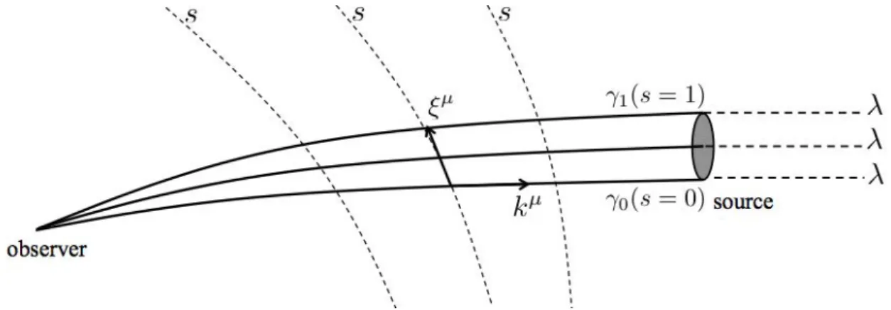
maintain-ing constant and varying s, one gets another collection of curves (which are not geodesics in general). The separation vectors ⇠µ _{= @}

sxµ are tangent to this

col-lection of curves and establish a connection between the geodesics. Besides, the vectors kµ= @ xµare tangent to the null geodesics (see figure 1.3 and more details in the paper presented in section 1.5).

Figure 1.3: A geodesic bundle.

Let us define the acceleration of the separation vector: D2⇠µ

D 2 =r⌫

⇣

k r ⇠µ⌘k⌫. (1.36)

In a flat spacetime, it is zero because in that case geodesics are straight lines so the variation of ⇠µ with is necessarily linear. Hence, a non zero acceleration reveals a curvature. In general relativity, it means that one expects this acceleration to be proportional to the Riemann tensor20Rµ _⌫. Noticing that k r ⇠↵ _{= ⇠} _{r k}↵ _and

using the geodesic equation k⌫_r⌫kµ= 0, one can see that the quantity ⇠µkµis

con-served along the geodesic 0

✓

d (⇠µkµ)

d = 0

◆

. Consequently, one can parametrize 19_{An affine parameter} _{is a parameter defined so that the geodesic equations governing the}

behavior of geodesics described by x↵( ) take the form d

2_x↵ d 2 + ↵ µ⌫ dxµ d dx⌫ d = 0. 20_{By definition, R}µ ⌫↵ = @↵ µ⌫ @ µ⌫↵+ µ↵ ⌫ µ ⌫↵. 25

(28)

the curves so that, on 0, ⇠µ and kµ are always orthogonal (⇠µkµ= 0). The same

properties allow to compute the acceleration of 1 with respect to 0(see e.g. [131]):

D2⇠µ

D 2 = ⇠ R

µ ⌫k k

⌫ _. _(1.37)

It is the geodesic deviation equation.

Once projected on a judicious basis, it leads to the so-called Sachs equation and finally the separation vectors can be related to observables such as the luminosity distance (see our paper, section 1.5).

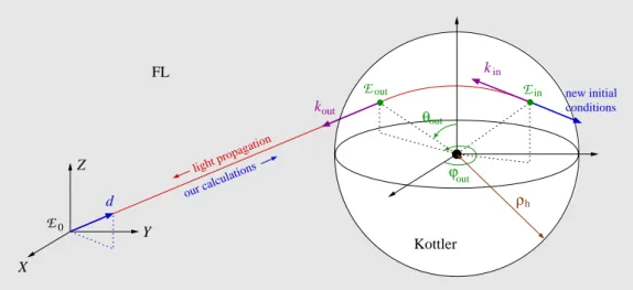
Strategy adopted to determine the light path

In practice, what we did to determine the light path between a source and an observer is to start from the observer (assumed to stand in the Friedmann-Lemaˆıtre region) and to reconstruct, step by step, the trajectory of photons back to the source. The first step is the identification of the coordinates corresponding to a photon leaving the last hole encountered before reaching the observer (resolution of the geodesic equation in the Friedmann-Lemaˆıtre metric). Next, the resolution of the Sachs equation gives the behavior of the separation vector. It is then necessary to switch to the Kottler metric to infer the deviation caused by the point mass inside the hole. Identification of the geodesics relies on two conservation laws which reflect that the Kottler metric is static21 and with a spherical symmetry. It gives the coordinates associated with the event corresponding to photons entering the last hole. Then the Sachs equation is integrated again and one goes back to the Friedmann-Lemaˆıtre metric. One can iterate this procedure for an arbitrary number of holes, until one assumes that the source has been reached. Throughout the whole calculation, the evolution of the wavenumber is also studied, which gives the evolution of the cosmological redshift of the source (by comparing the wavenumber at emission and reception times). Thanks to the resolution of the Sachs equation, the luminosity distance is also part of the traceable observables. Consequently, Hubble diagrams can be computed once the observation conditions, the distribution of the holes, the value of the point masses and the redshifts of the sources are specified (full details are given in section 1.5). Besides, they can be easily compared to what they would be in a configuration similar but with no hole.

21_{The fact that it is static is a consequence of Birkho↵’s theorem, see e.g. [}₆₉_].

(29)

1.4. Impact of inhomogeneities on cosmology

1.4 Impact of inhomogeneities on cosmology

Cosmological parameters are omnipresent in the equations of our study so the as-pect of Hubble diagrams strongly depends on them. We therefore introduced the quantities ⌦⇤= ⇤ 3H2 0 , ⌦m= 8⇡G⇢0 3H2 0 , ⌦K= K a2 0H02 , (1.38)

where an index 0 indicates that the quantity is evaluated at present time. ⌦⇤ is one

of the six cosmological parameters of the standard model of cosmology. It charac-terizes the amount of dark energy in the universe. According to [135], results from the Planck satellite lead to the 1 -constraint22_⌦

⇤= 0.686± 0.020 (the meaning of

“1 -constraint” is given below.). ⌦m characterizes the amount of non-relativistic

matter (and is related to the standard cosmological parameter !m via !m= ⌦mh2,

with h defined so that H0 = 100 h km.s 1). It is the sum of the amounts of

bary-onic matter and cold dark matter. Still from [135] and with the same precision, one estimates ⌦m= 0.315± 0.017. ⌦K indicates what the spatial curvature of the

uni-verse is. It is given by ⌦K= 1 ⌦⇤ ⌦m. Observational constraints are therefore

compatible with ⌦K= 0, which means that the universe can reasonably be assumed

to have a flat geometry.

On the one hand, we used our Hubble diagrams as mock data and tried to inter-pret them assuming a homogeneous and isotropic geometry. More precisely, we used the Chi-Square Goodness of Fit Test to estimate the values of the parameters (1.38) that best fit the resulting diagrams when the spacetime is entirely characterized by the Friedmann-Lemaˆıtre metric. Generally, this test summarizes the discrepancy between observed values O (here the mock data) and the values E expected under the model in question (here the homogeneous model). The generic formula is

2 ₌X

data

(O E)2

2 , (1.39)

where is an observational error bar23_{. The values of} 2 _{give the best fit, i.e.}

the values of E that best match observations, and confidence contours, i.e. areas in parameter space in which the parameters are expected to lie with a probability

22_{This estimation is yet highly model dependent.}

23_{In our study, we estimated} _{by imitating a real catalog of SNIa observations.} 27

(30)

1.4. Impact of inhomogeneities on cosmology

exceeding a given value24 (see e.g. [141] for more details). We found that the es-timated cosmological parameters can be very di↵erent from the actual parameters characterizing the Swiss-cheese spacetime in which we simulated light propagation. In other words, in some cases, the homogeneity assumption largely a↵ects the esti-mation of the cosmological parameters (see the detailed study in section 1.5).

Another test we performed is the estimation of the cosmological parameters of the Swiss-cheese model that best reproduce real observations. Using the same 2

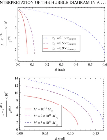
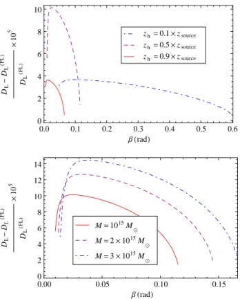
method, we found that replacing a Friedmann-Lemaˆıtre model by a Swiss-cheese one can in some cases induce a significant (regarding the accuracy intended by pre-cision cosmology, i.e. a few percent) di↵erence in the prediction of the parameters (see section 1.5). It required in particular to estimate analytically a luminosity distance-redshift relation of a Swiss-cheese universe. Evaluating such e↵ects is an important issue since the 2013 Planck results ([135]) highlighted a tension between the estimation of H0 and ⌦m from CMB observations and their estimation from

other observables, such as SNIa. In the paper presented in section 1.6, we demon-strate that Swiss-cheese descriptions make possible the reconciliation between the values of ⌦m inferred from Planck and from SNIa. This is illustrated in figure 1.4.

Besides, the 2015 Planck results ([137]) show that the estimation of H0 from

Planck is in fact consistent with its estimation from the recent “Joint Light-curve Analysis” sample of SNIa (constructed from the SNLS and SDSS supernovae data, together with several samples of low redshift supernovae, [20]).

24_{For a Gaussian probability distribution of the parameters, we call “1 -contours” the contours}

associated with a 68.3% probability, “2 -contours” the contours associated with a 95.4% probability and “3 -contours” the contours associated with a 99.73% probability.

(31)

1.5. Article “Interpretation of the Hubble diagram in a nonhomogeneous universe”

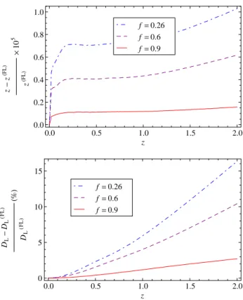
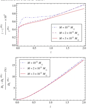
Figure 1.4: Comparison of the constraints obtained by Planck on (⌦m, h), [135],

and from the analysis of the Hubble diagram constructed from the SNLS 3 catalog, [86]. f is the “smoothness parameter”, which gives the ratio between the volume which is not in form of holes and the total volume. Hence, f = 1 corresponds to the Friedmann-Lemaˆıtre metric.

1.5 Article “Interpretation of the Hubble diagram in a

nonhomogeneous universe”

(32)

Interpretation of the Hubble diagram in a nonhomogeneous universe

Pierre Fleury,1,2,*He´le`ne Dupuy,1,2,3,†and Jean-Philippe Uzan1,2,‡

1_{Institut d’Astrophysique de Paris, UMR-7095 du CNRS, Universite´ Pierre et Marie Curie, 98 bis bd Arago, 75014 Paris, France} 2_{Sorbonne Universite´s, Institut Lagrange de Paris, 98 bis bd Arago, 75014 Paris, France}

3_{Institut de Physique The´orique, CEA, IPhT, URA 2306 CNRS, F-91191 Gif-sur-Yvette, France}

(Received 15 March 2013; published 24 June 2013)

In the standard cosmological framework, the Hubble diagram is interpreted by assuming that the light emitted by standard candles propagates in a spatially homogeneous and isotropic spacetime. However, the light from ‘‘point sources’’—such as supernovae—probes the Universe on scales where the homogeneity principle is no longer valid. Inhomogeneities are expected to induce a bias and a dispersion of the Hubble diagram. This is investigated by considering a Swiss-cheese cosmological model, which (1) is an exact solution of the Einstein field equations, (2) is strongly inhomogeneous on small scales, but (3) has the same expansion history as a strictly homogeneous and isotropic universe. By simulating Hubble diagrams in such models, we quantify the influence of inhomogeneities on the measurement of the cosmological parameters. Though significant in general, the effects reduce drastically for a universe dominated by the cosmological constant.

DOI:10.1103/PhysRevD.87.123526 PACS numbers: 98.80._{!k, 04.20.!q, 42.15.!i}

I. INTRODUCTION

The standard physical model of cosmology relies on a solution of general relativity describing a spatially homo-geneous and isotropic spacetime, known as the Friedmann-Lemaıˆtre (FL) solution (see e.g. Ref. [1]). It is assumed to describe the geometry of our Universe smoothed on large scales. Besides, the use of the perturbation theory allows one to understand the properties of the large scale struc-ture, as well as its growth from initial conditions set by inflation and constrained by the observation of the cosmic microwave background.

While this simple solution of the Einstein field equa-tions, together with the perturbation theory, provides a description of the Universe in agreement with all existing data, it raises many questions on the reason why it actually gives such a good description. In particular, it involves a smoothing scale which is not included in the model itself [2]. This opened a lively debate on the fitting problem [3] (i.e. what is the best-fit FL model to the lumpy Universe?) and on backreaction (i.e. the fact that local inhomogene-ities may affect the cosmological dynamics). The ampli-tude of backreaction is still actively debated [4–6], see Ref. [7] for a critical review.

Regardless of backreaction, the cosmological model assumes that the distribution of matter is continuous (i.e. it assumes that the fluid approximation holds on the scales of interest) both at the background and perturbation levels. Indeed numerical simulations fill part of this gap by deal-ing with N-body gravitational systems in an expanddeal-ing space. The fact that matter is not continuously distributed

can however imprint some observations, in particular regarding the propagation of light with narrow beams, as discussed in detail in Ref. [8]. It was argued that such beams, as e.g. for supernova observations, probe the space-time structure on scales much smaller than those accessible in numerical simulations. The importance of quantifying the effects of inhomogeneities on light propagation was first pointed out by Zel’dovich [9]. Arguing that photons should mostly propagate in vacuum, he designed an ‘‘empty beam’’ approximation, generalized later by Dyer and Roeder as the ‘‘partially filled beam’’ approach [10]. More generally, the early work of Ref. [9] stimulated many studies on this issue. [11–25].

The propagation of light in an inhomogeneous universe gives rise to both distortion and magnification induced by gravitational lensing. While most images are demagnified, because most lines of sight probe underdense regions, some are amplified because of strong lensing. Lensing can thus discriminate between a diffuse, smooth compo-nent, and the one of a gas of macroscopic, massive objects (this property has been used to probe the nature of dark matter [26–28]). Therefore, it is expected that lensing shall induce a dispersion of the luminosities of the sources, and thus an extra scatter in the Hubble diagram [29]. Indeed, such an effect does also appear at the perturbation level— i.e. with light propagating in a perturbed FL spacetime— and it was investigated in Refs. [30–35]. The dispersion due to the large-scale structure becomes comparable to the intrinsic dispersion for redshifts z > 1 [36] but this disper-sion can actually be corrected [37–42]. Nevertheless, a considerable fraction of the lensing dispersion arises from sub-arc minute scales, which are not probed by shear maps smoothed on arc minute scales [43]. The typical angular size of the light beam associated with a supernova (SN) is typically of order 10!7 arc sec (e.g. for a source of

*fleury@iap.fr

†_{helene.dupuy@cea.fr} ‡_uzan@iap.fr

(33)

physical size_{"1 AU at redshift z " 1), while the typical} observational aperture is of order 1 arc sec. This is smaller than the mean distance between any massive objects.

One can estimate [27] that a gas composed of particles of mass M can be considered diffuse on the scale of the beam of an observed source of size !s if M<

2_{# 10}!23M_$h2_ð!

s=1 AUÞ3. In the extreme case for which

matter is composed only of macroscopic pointlike objects, then most high-redshift SNeIa would appear fainter than in a universe with the same density distributed smoothly, with some very rare events of magnified SNeIa [27,44,45]. This makes explicit the connection between the Hubble diagram and the fluid approximation which underpins its standard interpretation.

The fluid approximation was first tackled in a very innovative work of Lindquist and Wheeler [46], using a Schwarzschild cell method modeling an expanding universe with spherical spatial sections. For simplicity, they used a regular lattice which restricts the possibilities to the most homogeneous topologies of the 3-sphere [47]. It has recently been revisited in Refs. [48] and in Refs. [49] for Euclidean spatial sections. They both constructed the associated Hubble diagrams, but their spacetimes are only approximate solutions of the Einstein field equations. An attempt to describe filaments and voids was also pro-posed in Refs. [50].

These approaches are conceptually different from the solution we adopt in the present article. We consider an

exact solution of the Einstein field equations with strong density fluctuations, but which keeps a well-defined FL averaged behavior. Such conditions are satisfied by the Swiss-cheese model [51]: one starts with a spatially homo-geneous and isotropic FL geometry, and then cuts out spherical vacuoles in which individual masses are em-bedded. Thus, the masses are contained in vacua within a spatially homogeneous fluid-filled cosmos (see bottom panel of Fig. 2). By construction, this exact solution is free from any backreaction: its cosmic dynamics is identi-cal to the one of the underlying FL spacetime.

From the kinematical point of view, Swiss-cheese models allow us to go further than perturbation theory, because not only the density of matter exhibits finite fluc-tuations, but also the metric itself. Hence, light propagation is expected to be very different in a Swiss-cheese universe compared to its underlying FL model. Moreover, the in-homogeneities of a Swiss cheese are introduced in a way that addresses the so-called ‘‘Ricci-Weyl problem.’’ Indeed, the standard FL geometry is characterized by a vanishing Weyl tensor and a nonzero Ricci tensor, while in reality light mostly travels in vacuum, where conversely the Ricci tensor vanishes—apart from the contribution of !, which does not focus light—and the Weyl tensor is nonzero (see Fig. 1). A Swiss-cheese model is closer to the latter situation, because the Ricci tensor is zero inside the holes (see Fig.2). It is therefore hoped to capture the relevant optical properties of the Universe.

Ricci = 0 Weyl = 0 Ricci = 0 Weyl = 0 SN Ia SN Ia Real Universe FL model

FIG. 1 (color online). The standard interpretation of SNe data assumes that light propagates in purely homogeneous and iso-tropic space (top). However, thin light beams are expected to probe the inhomogeneous nature of the actual Universe (bottom) down to a scale where the continuous limit is no longer valid.

Ricci = 0 Weyl = 0 Ricci = 0 Weyl = 0 SN Ia SN Ia FL model

Swiss−cheese model

FIG. 2 (color online). Swiss-cheese models (bottom) allow us to model inhomogeneities beyond the continuous limit, while keeping the same dynamics and average properties as the FL model (top).