Analysis of Aerosol-Cloud Interaction from Space

(1)

HAL Id: tel-01430153

https://hal.archives-ouvertes.fr/tel-01430153

Submitted on 9 Jan 2017

HAL is a multi-disciplinary open access

archive for the deposit and dissemination of sci-entific research documents, whether they are pub-lished or not. The documents may come from teaching and research institutions in France or abroad, or from public or private research centers.

L’archive ouverte pluridisciplinaire HAL, est destinée au dépôt et à la diffusion de documents scientifiques de niveau recherche, publiés ou non, émanant des établissements d’enseignement et de recherche français ou étrangers, des laboratoires publics ou privés.

Analysis of Aerosol-Cloud Interaction from Space

Lorenzo Costantino

To cite this version:

Lorenzo Costantino. Analysis of Aerosol-Cloud Interaction from Space. Geophysics [physics.geo-ph]. Université de Versailles et Saint-Quentin-en-Yvelines, 2012. English. �tel-01430153�

(2)

UNIVERSITE DE VERSAILLES SAINT-QUENTIN-EN-YVELINES

École Doctorale des Sciences de l’Environnement d’Ile-de-France - SEIF

Laboratoire des Sciences du Climat et de

l'Environnement (LSCE) – UMR 8212

THÈSE DE DOCTORAT

DE L’UNIVERSITE DE VERSAILLES SAINT–QUENTIN–EN-YVELINES

Spécialité :

Météorologie, océanographie physique et physique de l’environnement

Présentée par :

Lorenzo Costantino

Pour obtenir le grade de Docteur de l’Université de Versailles Saint-Quentin-en-Yvelines

Analysis of Aerosol-Cloud Interaction from Space

Soutenue le : 13 Janvier 2012

---Directeur de thèse :

François-Marie, Bréon

Devant le jury composé de : Rapporteurs :

Jérôme RIEDI Professeur à l'Université de Lille, chercheur au LOA

Jean-Claude ROGER Professeur à l'Université de Clermont-Ferrand, chercheur au LAMP

Examinateurs :

Philippe BOUSQUET Professeur à l'UVSQ, chercheur au LSCE

Francois-Marie BRÉON Chercheur au LSCE (directeur de thèse) Jean-Pierre CHABOUREAU Chercheur au Laboratoire d’Aérologie

(3)

(4)

Abstract

The aim of this work is to provide a comprehensive analysis of cloud and aerosol interaction over South-East Atlantic, to quantify the overall aerosol impact on the regional radiation budget. We used data from MODIS, PARASOL and CALIPSO satellites, that fly in close proximity on the same sun-synchronous orbit and allow for complementary observations of the same portion of the atmosphere, within a few minutes.

The main idea is to use CALIPSO vertical information to define whether or not aerosol and cloud layers observed by MODIS and PARASOL are mixed and interacting. We found evidences that, in case of interaction, cloud properties are strongly influenced by aerosol presence (first indirect effect). In particular, there is a decrease in cloud droplet effective radius and liquid water path with aerosol enhancement. On the other hand, we could not evidence any significant impact on the cloud reflectance.

We also analyzed the aerosol impact on precipitation (second indirect effect). In polluted low clouds over the ocean, we found evidence of precipitation suppression and cloud cover increase with increasing aerosol concentration. On the other hand, cloud fraction is shown to be affected by aerosol presence, even if pollution particles are located above cloud top, without physical interaction. This observation is interpreted as a consequence of the aerosol radiative effect.

Aerosol shortwave direct (DRF) and indirect (IRF) radiative forcing at TOA has been quantified, with the use of a radiative transfer model constrained by satellite observations. For the direct effect, there is a competition between cooling (negative, due to light scattering by the aerosols) and warming (positive, due to the absorption by the same particles). The regional six year (2005-2010), the spatial mean and the standard deviation is equal to -0.07±8.03 W/m² for DRF and -0.05±0.54 W/m² for IRF. Indirect forcing results from the balance of cloud albedo effect (-0.07±0.55 W/m²) and life time effect (0.02±0.12 W/m²). Total aerosol forcing is then negative (cooling) and equal to -0.12±8.02 W/m².

Résumé

Le but de cette thèse est de fournir une analyse exhaustive des interactions entre nuages et aérosols dans le Sud-Est de l'Atlantique, en quantifiant l'impact des aérosols sur le bilan radiatif régional en ondes courtes. Pour cet objectif, nous avons utilisé les données satellitaires de MODIS, PARASOL et CALIPSO, qui fournissent des observations complémentaires et quasi simultanées.

L'idée principale qui a permis une analyse originale est d'utiliser les observations du lidar CALIPSO pour identifier les cas pour lesquels les couches d’aérosols et nuages vues par MODIS et PARASOL sont en interaction (mélangées) et ceux pour lesquels ils sont clairement disjoints. Il ressort de cette analyse que les propriétés des nuages sont fortement influencées par l'interaction avec les aérosols (premier effet indirect). On observe une diminution du rayon efficace de gouttelettes et du contenu en eau sous l'effet d’une hausse de la concentration des particules polluantes. En revanche, nous n’avons pas mis en évidence une modification significative de la réflectance des nuages.

Lorsque les aérosols et les nuages sont mélangés, on observe aussi une diminution de l’occurrence des précipitations (second effet indirect) et l'augmentation de la couverture nuageuse. D'autre part, la fraction nuageuse est affectée par la présence d'aérosols, même si les particules de pollution sont situées au-dessus du sommet des nuages (sans interaction physique). Cette observation est interprétée comme étant une conséquence de l'effet radiatif des aérosols.

Pour quantifier le forçage radiatif direct et indirect des aérosols, nous avons utilisé un code de transfert radiatif rapide à onde courte, contraint par les observations satellitaires. Sur six ans (2005-2010), le forçage moyen et sa déviation standard sur toute la région sont égaux à -0.07±8.03 W/m² pour l'effet direct et -0.05±0.54 W/m² pour l'effet indirect. Ce dernier est déterminé par l'équilibre entre l'effet de la variation de l’albédo (-0.07±0.55 W/m²) et celui de la couverture nuageuse (0.02±0.12 W/m²). Le forçage total est donc négatif (refroidissement) et égal à -0.12±8.02 W/m².

(5)

(6)

Analyse des interactions entre aérosol et nuages par

mesures télédétectées

(10)

Synthèse

Ce travail porte sur l’analyse des interactions entre les aérosols et les nuages, avec, in-fine, l’objectif de quantifier l’impact radiatif des aérosols, en incluant l’effet indirect via la modification des caractéristiques microphysiques et macrophysiques des nuages. Pour mener à bien cette étude, nous avons utilisé des données de télédétection spatiale acquises par les capteurs MODIS, PARASOL et CALIPOP. Notre travail est focalisé sur une zone du Sud-Est Atlantique (au large de l’Angola) qui est une région particulièrement intéressante car sous le vent de l’Afrique et deux zones émettrices d’aérosol de brûlis, ainsi que des poussières d’origine saharienne. La principale originalité du travail, par rapport à d’autres études publiées ces dernières années, a été d’utiliser les mesures du lidar spatial CALIPSO, afin de pouvoir analyser la position respective des aérosols et des nuages. Nous avons mis en place une base de données statistiques donnant les distributions de divers paramètres décrivant les couches d’aérosols et de nuages, couplée à un code de transfert radiatif. Ce travail permet de tester un certain nombre d’hypothèses car, comme le signale le dernier rapport de l’IPCC, l’effet radiatif des aérosols et des nuages reste assez mal connu. Pour mieux suivre la démarche scientifique de ce sujet, le manuscrit se décompose en 8 chapitres (hors Introduction et Conclusion).

Dans le Chapitre 1, on pose les bases théoriques et les diverses principes de la formation, en présence d’aérosol, d’un nuage et des précipitations associées.

Dans le Chapitre 2, lui aussi introductif, nous abordons l’aspect télédétection spatiale. Alors que la première partie de ce chapitre est plus historique, la deuxième partie décrit comment les données satellitaires acquises par MODIS, PARASOL et CALIOP sont utilisées à des fins d’inversion des propriétés des nuages et des aérosols.

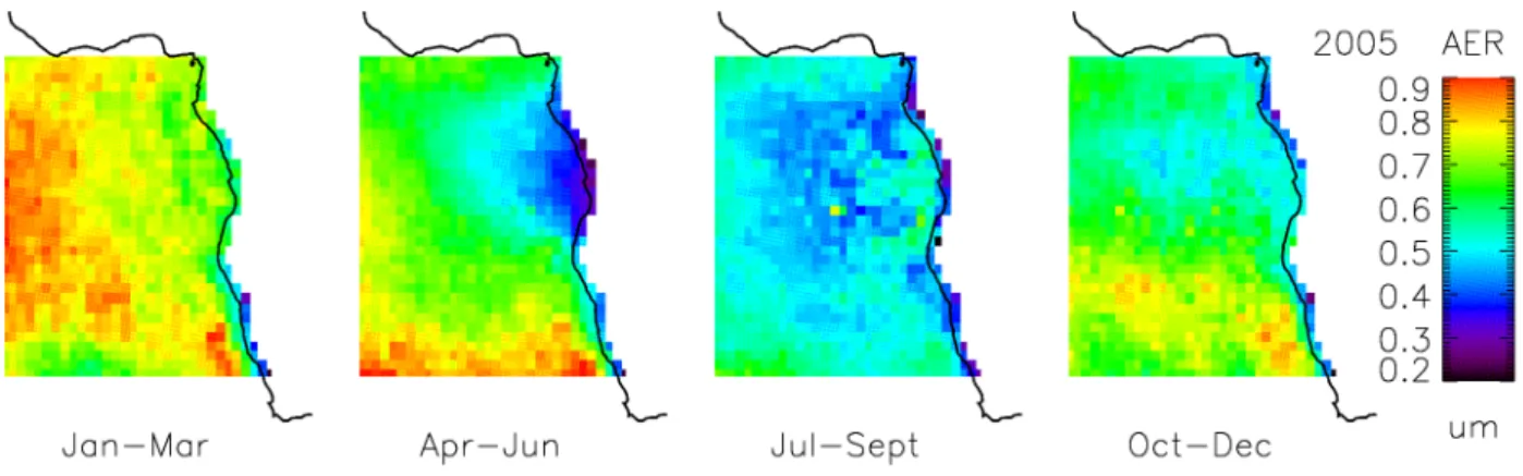
Le contenu du Chapitre 3 constitue une première approche vers l’analyse des interactions aérosols-nuages. A travers l’analyse des données MODIS sur les feux de forêt, on observe que la zone du Sud-Est Atlantique est une zone particulièrement favorable pour l’étude de ces interactions, étant donné l’injection saisonnière dans l’atmosphère d’aérosols fins générés lors des processus de brûlis. Ensuite, l'analyse s’attelle à une étude saisonnière (4 trimestres) et inter-annuelle (2005-2010) des propriétés optiques des aérosols et des nuages (données MODIS). On observe ainsi une très forte saisonnalité, tant pour les aérosols que pour les nuages, liée (1) au transport d’aérosols de brûlis au large de l’Angola lors de la période Juillet-Septembre, et (2) au transport d’aérosols désertiques dans le golfe de Guinée lors de la période Janvier-Mars (Figure 1). Par contre, les variations inter-annuelles sont limitées.

(11)

Figure 1: Moyenne saisonnière de l'indexe aérosol (AI), pour le 2005. AI est proportionnel à la concentration d’aérosol dans atmosphère.

Les résultats obtenus montrent une relation nette entre charge en aérosols et paramètres nuageux. Cependant, il apparaît que les corrélations observées peuvent être, au moins en partie, liées à effet météorologique qui couplerait les deux variables de manière fortuite. Une étude plus fine, incluant une analyse des structures temporelles et de la position respective des couches aérosols et nuages, est nécessaire.

Le Chapitre 4 fait un état de l’art, tant théorique qu’expérimental, de l’effet des aérosols sur les nuages et les précipitations associées.

Le Chapitre 5 se focalise sur la corrélation entre l’indice aérosol (AI) et le rayon des particules nuageuses (CDR), toujours sur la zone concernée et à partir de données MODIS. Dans un premier temps (données MODIS), on retrouve bien le même type de relation entre ces 2 paramètres que celle attendue par la théorie (le logarithme du CDR est inversement proportionnelle au logarithme de l’AI) mais avec un coefficient de linéarité très différent. On émet alors l’hypothèse que cela est dû à un problème de mélange aérosols-nuages. Grâce à la méthode MPC proposée, combinant les données de MODIS, PARASOL et CALIOP, on montre qu’il faut distinguer les cas pour lequel la couche d’aérosols est mélangée avec la couche de nuages des cas pour lesquels les 2 couches ne sont pas mélangées (Figure 2). Dans le premier cas (couches en interaction), la relation statistique moyenne est conforme à la théorie et aux résultats existants ; dans le deuxième cas, il n’existe quasiment pas de corrélation. Par conséquent, il est démontré que les aérosols de brûlis ont un effet important sur la microphysique des nuages, et que l’impact moyen observé est cohérent avec les prédictions théoriques [Costantino and Bréon, 2011].

(12)

Figure 2: Relations entre le logarithme du CDR et le logarithme du AI, à travers une combinaison des données MODIS (AI), PARASOL (CDR) et CALIOP. L'information verticale apportée par CALIPSO permet de distinguer entre le cas pour lequel les couches d’aérosol et nouages sont mélangées (rouges) du cas pour lequel les 2 couches ne sont pas mélangées (bleu).

Le Chapitre 6 s’inscrit dans la continuité du chapitre précédent, en poursuivent l'étude de l’impact des aérosols de brûlis sur la microphysique des nuages à travers, cette fois, l'analyse de corrélations entre l’indice aérosols (AI) et le rayon des particules nuageuse (CDR), puis l’épaisseur optique des nuages (COT), et enfin le contenu intégré en eau condensée (LWP). Ces deux dernières relations sont, à ce jour, peu documentées et peu quantifiées. Pour cela, on développe cette fois la MMC méthode (MODIS, MODIS, CALIOP) afin de découpler les cas atmosphériques liés aux processus de météorologie locale et ceux des réelles interactions aérosols-nuages. Parallèlement, on confirme la synergie des instruments spatiaux en comparant le rayon des particules nuageuses (MODIS-PARASOL) et l’épaisseur optique des aérosols (MODIS-CALIOP).

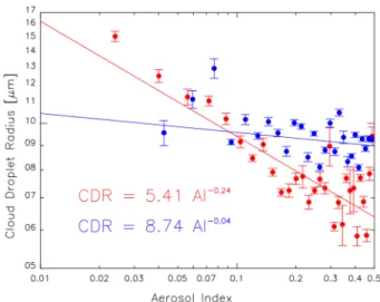
Les résultats de la méthode MMC sont de plusieurs ordres. Tout d’abord, on montre que les interactions aérosols-nuages semblent largement dominer les effets météorologiques locaux. Cela permet d’appréhender concrètement l’effet Twomey: en cas de mélange le logarithme du CDR est inversement proportionnelle au logarithme du AI (Figure 3). On trouve aussi que la quantité en eau des nuages (LWP) décroit avec l’AI, en cas d'interaction entre les couches d’aérosol et de nuage (ce qui n’est pas attendu à priori). Après analyse, ce résultat est interprété comme résultant de la faible humidité relative de la masse d’air transportant l’aérosol et qui se mélange à celle du nuage (Figure 4). On montre enfin que l’AI n’est que très peu corrélé avec l’épaisseur optique (COT) des nuages pollués (Figure 5), ce qui aura son importance pour le calcul des impacts radiatifs.

Malgré que le LWP ne suit pas la théorie de Twomey, l'étude menée dans ce chapitre montre que la concentration des aérosols a un impact sur le cycle de vie des nuages et que donc

(13)

l’efficacité radiative des aérosols dépend du LWP.

Figure 3: Relations entre le logarithme du CDR et le logarithme du AI, à travers une combinaison des données MODIS (AI), MODIS (CDR) et CALIOP. Le cas pour lequel les couches d’aérosol et nouages sont mélangées est indiqué en rouge, le cas pour lequel les 2 couches ne sont pas mélangées en bleu.

Figure 4: Relations entre le logarithme du LWP et le logarithme du AI, à travers une combinaison des données MODIS (AI), MODIS (LWP) et CALIOP. Le cas pour lequel les couches d’aérosol et nouages sont mélangées est indiqué en rouge, le cas pour lequel les 2 couches ne sont pas mélangées en bleu.

(14)

Figure 5: Relations entre le logarithme du COT et le logarithme du AI, à travers une combinaison des données MODIS (AI), MODIS (COT) et CALIOP. Le cas pour lequel les couches d’aérosol et nouages sont mélangées est indiqué en rouge, le cas pour lequel les 2 couches ne sont pas mélangées en bleu.

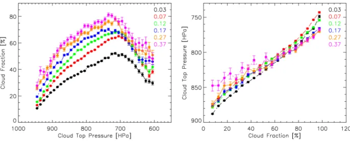
Le Chapitre 7 s’attelle à l’impact des aérosols sur le cycle de vie des nuages. Dans un premier temps, après un rappel théorique sur l’inhibition possible des précipitations due à la présence des aérosols, on met en évidence la diminution des précipitations des nuages pollués par les aérosols de brûlis dans la zone géographique considérée, pour le cas d’une couche d’aérosols mélangée avec les nuages. Pour COT > 10, les nouages pollués montrent une relation exponentielle entre CDR et COT moins faible que dans le cas des nuages propres (Figure 6), ce qui peut indiquer une inhibition des précipitations. Dans un deuxième temps (Figure 7, gauche), on confirme l’hypothèse (sur la durée de vie des nuages) selon laquelle une augmentation de la concentration en aérosols engendre une augmentation de la fraction nuageuse (CLF) selon une structure horizontale, paramétrée par la pression au sommet des nuages (CTP). Puis, on montre que les aérosols n’affectent pas, par contre, la structure verticale des nuages (Figure 7, droite). Dans une dernière partie, on indique, à partir de données MODIS et CALIOP, que l’effet radiatif des aérosols (aérosol-nuages pas mélangés) est plus important que l’interaction aérosols-nuages elle-même sur la durée de vie des nuages (Figure 8).

(15)

Figure 6: Relations entre CDR et COT, à travers une combinaison des données MODIS (AI), MODIS (COT) et CALIOP. Le cas pour lequel les couches d’aérosol et nouages sont mélangées est indiqué en rouge, le cas pour lequel les 2 couches ne sont pas mélangées en bleu.

Figure 7: (gauche) Relation entre le CLF (MODIS) et le CTP (MODIS), pour différentes valeurs de l'indexe d’aérosol (MODIS).(droit) Relation entre le CTP et le CLF, pour différentes valeurs de l'indexe d’aérosol.

(16)

Figure 8: Coefficient de la régression linéaire entre le logarithme du COT et le logarithme du AI, en fonction du développement vertical des nuages, qui augmente quand CTP diminue. Le cas pour lequel les couches d’aérosol et nouages sont mélangées (interaction) est indiqué en rouge, le cas pour lequel les 2 couches ne sont pas mélangées (effet radiatif) en bleu.

Le dernier chapitre (Chapitre 8) aborde les aspects radiatifs des aérosols à travers leurs effets direct et indirect au sommet de l’atmosphère à l’aide d’un modèle de calcul rapide du transfert radiatif.

Pour l’effet direct, on sait que les principales sources d’incertitude sont la valeur de l’albédo de simple diffusion (SSA) et la distribution verticale des aérosols. Nous avons donc mis une attention particulière à ces deux paramètres, en proposant une paramétrisation du SSA avec le type d’aérosols observés, et en utilisant les statistiques de distribution verticale des aérosols et des nuages provenant de CALIOP.

On trouve une forte variabilité saisonnière des impacts directs moyens sur le Sud-Est Atlantique de l’ordre de -5 W.m2_{(refroidissement lors du premier trimestre en présence d’aérosols}

désertiques) à +6 W.m2_{(réchauffement lors du troisième trimestre en présence d’aérosols de}

brûlis) avec des maxima allant respectivement de -25 à +47 W.m2 _{(Figure 9), ce qui n’est pas}

anodin. Ces résultats, pas forcément attendus, conduisent à une interprétation des diverses hypothèses utilisées par la communauté.

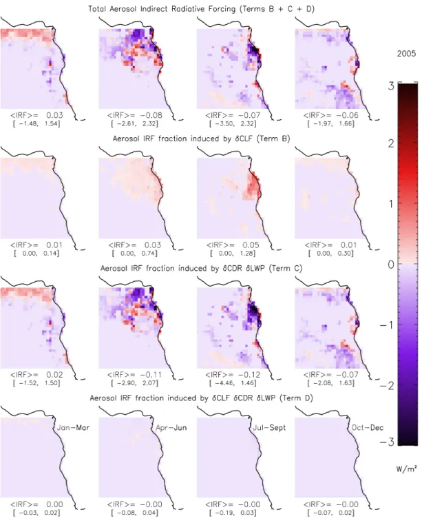
Le calcul des effets indirects (décomposés en 3 termes ici) montrent que ceux-ci sont d’un ordre inférieur ; de +0.02 W.m2₍₂ième_{trimestre) à -0.09 W.m}2₍₄ième_{trimestre) avec des valeurs}

maximales allant localement de -4 à +4 W.m2 _{(Figure 10). Cela peut paraître faible mais}

localement elles ne sont pas forcément négligeables au regard des valeurs globales. On montre donc, que l’effet direct prime largement sur l’effet indirect sur le Sud-Est Atlantique.

Par ailleurs, sur l’ensemble du jeu de données, l’impact radiatif sur la zone étudiée est faible (-0.07 W.m2_{en direct et -0.05 W.m}2_{en indirect) et conduit à un refroidissement de -0.12 W.m}2

(17)

entre les impacts positifs et négatifs selon les zones. Localement, les effets sont beaucoup plus forts.

En conclusion, nous avons utilisé dans cette thèse un grand nombre d’observations spatiales, passives et actives, pour caractériser les distributions spatio-temporelles des aérosols et des nuages sur l’Atlantique Sud-Est. Plusieurs relations entre charge en aérosols et paramètres nuageux ont été établies de manière statistique à partir de ces distributions. La difficulté principale est de distinguer les corrélations causales (liée à un processus d’interaction aérosol-nuage) de celles qui sont fortuites (Variations météorologiques conduisant à des corrélation non causales). Dans le but d’identifier les relations causales, nous avons utilisé les mesures actives du lidar CALIPSO qui permettent d’identifier la position respective des couches d’aérosols et de nuages. Nous avons montré que l’impact des aérosols sur la microphysique des nuages est indéniable (décroissance du rayon moyen des gouttes en présence d’aérosols) mais que l’effet sur l’albédo du nuage était insignifiant. Ce résultat apparemment paradoxal est dû à une décroissance du contenu en eau du nuage en présence d’aérosols. Nous pensons qu’il s’agit là d’un effet de mélange de l’air sec (qui contient les aérosols) avec le nuage, conduisant à une diminution de son contenu en eau.

Les relations obtenues sur la dépendance aérosol-nuage, et les distribution tri-dimensionnelles des couches ont ensuite été utilisées dans un code de transfert radiatif afin d’estimer les forçages radiatifs, directs et indirects, des aérosols. Sur la zone d’étude, l’effet est plus faible qu’attendu, compte tenu de la charge importante en aérosols. En fait, les valeurs obtenues résultent d’une compensation entre des effets forts positifs (absorption, en présence de nuages sous-jacents) et des effets forts négatifs (diffusion, en ciel clair). En ce qui concerne les effets indirects, on trouve là encore des effets plus faibles qu’attendus, du fait de la compensation entre l’impact sur la microphysique (décroissance de la taille des gouttes) et diminution du contenu en eau.

Ces résultats pourraient être utilisés pour évaluer les modèles Chimie-Climat qui sont utilisés pour quantifier l’effet radiatif des aérosols à l’échelle globale, en particulier dans le cadre du prochain rapport de l’IPCC (Fifth Assessment Report; AR5).

(18)

Figure 9: Moyenne saisonnière de l'impact direct sur le Sud-Est Atlantique, pour le 2005.

Figure 10: Moyenne saisonnière de l'impact indirect total sur le Sud-Est Atlantique pour le 2005 et décomposés en 3 termes: celui du à la variation du CLF (terme B), à la variation du CDR et COT (terme C), à la variation du CDR et COT dans la fraction nuageuse augmenté par l'effet de l'interaction entre nuages et aérosol (terme D).

(19)

Figure 11: Histogramme de l'impact direct, indirect et total sur le Sud-Est Atlantique, sur l’ensemble des données de 2005 au 2010. La moyenne sur l'effet indirect, égale à 0.19W/m², est calculée sur les seuls valeurs différents de zéro. Si on considère tout la région, le forçage moyen est égale à -0.05 W/m².

(20)

Introduction

Anthropogenic aerosols are part of the Earth climate system. The consequence of their interaction with clouds is the primary uncertainty on anthropogenic forcing (Intergovernmental Panel on Climate Change, 2007). They originate from urban and industrial pollution or smoke from fires and may affect cloud microphysics, cloud life cycle, precipitation formation and the overall quantity of sunlight radiation reflected to space.

Aerosol effects on clouds and Earth's energy balance

Most aerosols are highly reflective compared to the molecular scattering of clean atmosphere. An increase in their concentration can raise planet's albedo and increase the portion of solar radiation reflected to space. Such effect reduces the amount of energy entering into the Earth climate system and the amount of solar radiation reaching planet surface, with respect to an aerosol-free atmosphere. This direct impact on Earth radiative balance cools the surface and reduces the global warming resulting from the increase of greenhouse gases.

Aerosols from smoke and urban haze contain organic compounds and black carbon, a strong absorber of solar radiation. The consequence of their interaction with incoming sunlight is twofold, cooling the surface and heating the atmosphere, with a warming rate that depends on the aerosol chemical composition and the albedo of the underling surface (clouds, ocean, land, etc). This mechanism, known as aerosol direct effect (ADE), may reduce the vertical temperature gradient of the atmosphere and cause a decline in evaporation and cloud formation (Hansen et al. 1997; Ackerman et al., 2000).

Aerosol can also interact with clouds during their formation process (cloud nucleation), acting as CCN (Cloud Condensation Nuclei). In polluted region, the increase in aerosol particle concentration can enhance cloud droplet number concentration (CDNC), resulting in a reduction of mean droplet size (Bréon et al. 2002). For the same spatial distribution of liquid water, a cloud made of more numerous small droplets, reflects more than a cloud with fewer and larger droplets (Twomey, 1974; Twomey, 1977). Thus, an increase in aerosol load can lead to an increase in cloud reflectance, if cloud water amount remains constant. This process, known with the name of 'Twomey's effect' or 'first aerosol indirect effect' (AIE #1), produces a negative forcing on Earth radiative balance with a net cooling effect on climate. The importance of anthropogenic aerosol impact on cloud albedo has been acknowledged by the Intergovernmental Panel on Climate Change (IPCC), 2007, with large uncertainty.

A strong feedback can rise from the higher concentration of smaller droplets in polluted clouds, where coalescence processes are suppressed and precipitation efficiency decreases (Albrecht, 1989). Inhibition of precipitation may increase cloud life time and cloud liquid water path, with

(21)

aerosol indirect effect' (AIE #2) would ultimately modify cloud cover, in a way that is still poorly quantified.

The cooling effect of polluted clouds (first indirect effect) is still not completely characterized, while aerosol modification of cloud dynamics and precipitation patterns (second indirect effect) is even more uncertain. In fact, whereas aerosol impact on cloud microphysical is has been well established on global scale, the liquid water path response is far from being well understood. A number of studies show a significant positive correlation between liquid water path and CCN (Quaas et al. 2008; Loeb and Shuster, 2008, Quaas et al. 2009), some others a small but positive correlation (Nakajima et al., 2001; Sekiguchi et al., 2003), some others a negative correlation (Twohy et al. 2005; Matsui et al. 2006, Lee at al. 2009) while others affirm that this relationship can be positive or negative (Han et al. 2002) and depends on cloud regime (Lebsock, 2008) or only on meteorological variations (Menon et al. 2008).

These are complex processes to simulate in a model. In addiction, aerosol concentration and composition may largely vary in space and time. Long-term regional and global observations from satellites, ground stations and air-borne instruments are often needed to constraint models. At present days, we have limited direct observations of aerosol-cloud interaction impact on climate and state-of-the-art model estimates present large disparities (Lohomann and Feichter, 2005).

Many studies (Stevens and Feingold, 2009) agree on the fact that aerosol optical depth and low cloud incidence correlate well with the same meteorological parameters (surface wind speed, atmospheric moisture, stability, etc..). Local variations of one of these parameters can results in apparent correlations between aerosol and cloud retrievals. Therefore, one of the first and most difficult targets of present time research is to separate the impact of meteorology from aerosol-induced effects.

South-East Atlantic region is particularly suited to investigate radiative and physical effects of aerosol-cloud interaction. Large amount of aerosol load, produced from fires in Southern Africa, are injected into the atmosphere and transported by trade wind over Atlantic ocean, where a semi-permanent low cloud field is present. For their physical and chemical properties aerosols from biomass burning are very efficient CCN. In the absence of wet scavenging they can stay suspended in the atmosphere for days and weeks and be transported to considerable distances. In most cases, aerosol remains confined in the elevated layers of the atmosphere above cloud deck, well separated from it. As a consequence of their strong absorption properties, biomass burning particles may largely warm the atmosphere and produce a net positive forcing at the Top Of the Atmosphere (TOA). When aerosol gets mixed with the underlying cloud layer, the effect of their physical interaction can be statistically quantified by long term satellite observations.

(22)

Thesis structure and objectives

In this work, we perform a comprehensive analysis of the interaction between aerosol and warm clouds, in order to evaluate direct and indirect effects on South-East Atlantic radiative budget. Radiative forcing is considered the most simple and straightforward measure for the quantitative assessment of climate change mechanisms (Forster et al., 2005).

In Chapter 3 we study aerosol-cloud spatial and temporal variability over the area of interest, during 6 years of satellite observations. The first goal of this work has been to verify the expected aerosol effect on cloud microphysics. In Chapter 5 and Chapter 6, we quantify the decrease in cloud droplet radius with increasing aerosol concentration. In Chapter 6, we also investigate the expected increase in cloud optical thickness and cloud albedo as a consequence of droplet size diminution (AIE #1), as predicted by Twomey's hypothesis in case of constant liquid water path. Then, we analyze the liquid water path and cloud cover response to aerosol invigoration (AIE #2) and, in Chapter 7, we look for experimental evidence of precipitation suppression in polluted clouds. We quantified the strength of aerosol-induced effect with particular care in neglecting false correlations coming from local meteorology.

Chapter 8 focuses on the quantification of aerosol (and cloud) impact on the shortwave atmospheric radiation budget, over South-East Atlantic. We making use of the Rapid Response Transfer Model (RRTM_SW). We firstly deduced the shortwave radiative forcing due to the direct effect of aerosol on solar radiation, which depends on the aerosol optical properties coupled with the optical properties of its underling surface (ocean or clouds). Consequently we quantified the radiative forcing coming from the indirect effect of aerosol on cloud structure, which alters the way clouds interact with solar and thermal infrared radiation.

We use several aerosol and cloud parameters acquired from different satellite sensors: CALIOP lidar on board the CALIPSO satellite (for aerosol-cloud top and bottom layer altitudes), MODIS instrument on board of AQUA satellite (for cloud droplet radius, liquid water path, top pressure, cloud and aerosol optical depth, aerosol Angstrom coefficient, sea surface temperature), POLDER instrument on board of PARASOL satellite (for cloud droplet radius). Aerosol and cloud statistics are performed from co-located and time-coincided retrievals of the three A-train satellites, that fly in close proximity along the same orbit.

The main strategy of this work is to use CALIPSO data to analyze whether or not aerosol and cloud layers are mixed and interacting, in order to differentiate into two different classes the vertical integrated measurements of MODIS and PARASOL. For a given spatial location, if aerosol and cloud layers overlap or their altitudes are very close (within a certain threshold) they are considered interacting. In that case, a change in cloud properties with respect to a variation in aerosol concentration is interpreted as an aerosol driven process. On the other hand, if aerosol and cloud layers are well separated, the observed cloud change is considered as induced by other causes than cloud-aerosol interaction. This technique allows, to a certain degree, to isolate aerosol-induced effects from meteorology and obtain more reliable estimates of aerosol impact on clouds, than simple statistical satellite-based relationships between

(23)

(24)

Chapter I – Principles of cloud and precipitation formation

1.1 Cloud Nucleation and role of Aerosol as CCN

The first condition for cloud formation is supersaturation of water vapor. Supersaturation is the measure of the excess of water vapor above 100% Relative Humidity (RH) (Twomey, 1977a), so that 101% RH is equal to 1% supersaturation. However, supersaturation required to create water droplet by collision of water vapor molecules (homogeneous nucleation) greatly exceeds supersaturation values of the atmosphere. The kinetic theory of homogeneous nucleation predicts that a RH values of 300% to 800% are needed for a cloud of droplets to form by the growth of small clusters of water molecules (embryos) into droplets (Pruppacher and Klett, 1997; Vehkamäki, 2006). This means that clouds form by a different mechanism, (heterogeneous nucleation) according to which water vapor condensates upon a subset of atmospheric aerosols at supersaturation levels usually achieved in clouds (0,1 – 1%), much lower than those needed for heterogeneous nucleation.

Since the particles which serve as nuclei have sharply curved surfaces, a greater partial pressure is required to prevent evaporation from the particle surface than for a flat surface (Hind, 1982). This phenomenon is called Kelvin effect and it is described by the Kelvin equation which relates the saturation ratio (actual partial pressure of vapor divided by the saturation vapor pressure for a flat liquid) required for equilibrium above a droplet and the droplet size for a pure liquid (usually water) S_r= p p_s=exp ( 2 σ M ρRT r) (1) Sr = supersaturation ratio

ps = saturation vapor pressure for a flat liquid surface

p = actual partial pressure of vapor σ = surface tension of the liquid M = molecular weight of the liquid ρ = density of the liquid

r = Kelvin equilibrium particle radius R = ideal gas constant

T = absolute temperature

At the same time, in case of soluble CCN, the presence of a dissolved salt in water lowers the equilibrium vapor pressure above the water surface allowing activation to occur at a lower supersaturation with a soluble nucleus than with an insoluble one (Hinds, 1982). This process

(25)

When a droplet evaporates, the Kelvin effect increases the vapor pressure due to the increase in the surface curvature of the droplet but at the same time the concentration of salt in the droplet increases (total amount of salt remains constant). These are the two competing factors controlling the relationship between the saturation ratio and the particle size required for growth, which can be couplet together in a single equation (Köeler equation)

S_r= p p_s=

(

1+ i m_sM_w M_s4 3πρwr 3

)

−1 exp

(

2 σwMw ρ_wR T r

)

(2)

ms = mass of the dissolved salt

Ms = molecular weight of the dissolved salt

Mw = molecular weight of the water

σw= surface tension of the water ρw = density of the water

i = numbers of ions each molecule of salt forms r = particle radius

1.2 Köeler curves

This equation has not analytic solutions and a number of text provide a simplified form (expanding and taking only the firm therms of the expansion). If r is not too small it becomes

S_r=1+ A

r+ B

r3 (3)

A=2 σwMw

RT ρ Kelvin curvature term B= ϵi m Mw

M_s4

3π ρw

Raoult (solute) term

ε = soluble mass fraction of dry particle.

Equation 2 assumes that the solute is completely soluble (so that droplet is assumed to be homogeneous) and that the surface tension and density of the growing droplet are equal to those of water . Atmospheric aerosol are not always completely soluble and Hanel (1979) proposed a the introduction in Raoult term of the soluble mass fraction of the dry particle. It is very interesting to study the Köhler curves given by the latter equation as a function of droplet radius, keeping constant all other parameters. For very small particles the equilibrium saturation

(26)

ratio is under the unity (p < ps) allowing the presence of stable droplet of small size also if

supersaturation condition is not satisfied. Beneath the peak value of supersaturation if the relative humidity increases slightly, the droplet will grow slightly along the curve. If the relative humidity drops, the droplet will evaporate slightly until the vapor pressure over the droplet surface is in equilibrium with the ambient vapor pressure. Particles on the ascending part of the curve are called haze. If the relative humidity is increased up the supersaturation peak, the droplet will grow to a critical radius and the particle is said to be activated. Beyond this critical point, the increase in droplet radius is no more dependent on an increase in ambient relative humidity and water will continue to condense onto the droplet (hence the droplet will continue to grow) for a sufficient source of water vapor. Aerosol upon which cloud droplets form and get activated, are called cloud condensation nuclei.

The dependence of activation on aerosol dry size is shown in figure 1, where Köhler (activation) curves are shown for a range of dry diameter of two salt particles frequently assumed as CCN, ammonium sulphate and sodium chloride, (NH4)2 SO4 with solid line, NaCl with dashed line.

This figure show the differences in the supersaturation as a function of both the chemical composition and dry size of a particle (Raoult and Kelvin effects) for completely soluble particles and containing 50% by mass insoluble core.

Figure 1: Köhler (activation) curves for a range of dry diameter of salt particles ((NH4 )2 SO4 with solid line, NaCl with dashed line) and for 200 nm particles containing 50% by mass insoluble core (magenta). From McFiggans et al. (2006).

For a given aerosol composition, the larger is the size of a particle that serve as CCN, the more readily it gets wet by water and the greater is its solubility, the lower is the supersaturation at which the particle can serve as CCN and let star the cloud nucleation process. Pyrogenic organic emissions (biomass burning aerosol) with their relatively high solubility ave a key role

(27)

as CNN. The inorganic component (minor component)is made up of some insoluble dust and ash material, and soluble salts, and about half of the organic matter (major component) is water soluble (Reid et al. 2005; Decesari et al. 2006).

1.3 Particle growth and precipitation formation in warm clouds

When a air parcel rises, it expands and cools, so that it may reach saturation with respect to water. If it keeps cooling by a further lift, it may reach supersaturation values that begin to activate the most efficient CCN (the ones that need the lowest values of supersaturation) and cloud droplets form from the water vapor in excess of saturation. The cloud number concentration is equal to the number concentration of activated CCN. Yet from pioneering works of Squires (1958), Twomey and Warner (1967), Warner and Twomey (1967), and then confirmed in more recent 'in situ' observation (Garrett and Hobbs, 1995) and satellite images (Coakley et al. 1987; Durkee et al., 2000, 2001), it has been recognized that cloud droplet number concentration for clouds forming in clear environment have generally cloud droplet concentrations much lower than clouds forming in polluted atmosphere. Droplet concentration of cumulus clouds over ocean are generally lower than 100 cm-3, while clouds in polluted environment can reach values up to 1000 cm-3 (Squires, 1958)

Growing particles consume the disposable water vapor, so that the supersaturation begins to decrease, haze droplets to evaporate and only activated droplet continue to grow by condensation. Clouds forming at a temperature above 0 C are called warm clouds and are composed by liquid water only. In that case particle growth can be for condensation or collision

coalescence processes.

1.3.1 Condensation growth

The rate of mass (M) grow with time (t) for condensation can be established from the equation

dM

dt =4 π x

2_Dd ρm

dx (4)

where D (m²/s) is the coefficient of molecular diffusion and ρm the density of water molecules at

the position x. Equation 4 leads, with some manipulations and approximations, to the analytical expression of grow rate

(28)

rdr= A dt (5)

Where the term A= D Srρm

ρ_w can considered approximately constant. Equation 5 can be integrated to give

r ≈ At1/ 2 (6)

indicating that in the firsts instant after activation particle size grows rapidly, but rate of grow strongly decrease with time as particle size increase.

Theoretical calculation of Howell (1949) show that droplets growing by condensation approach a monodispersed size distribution after just 100 seconds after their activation. Typical droplet radius few hundreds meters above cloud base of non precipitating clouds, after 5 minutes from activation, is approximately 10 µm assuming condensations growth. This mechanism is too slow to produce rain droplets with typical radii of 1 or 2 millimeters.

1.3.2 Collision-coalescence process

Precipitation formation is given by collision-coalescence processes, that are based on the rapid growth of a cloud droplet as it falls through the cloud, colliding with the cloud droplets laying in its trajectory and forming a unique larger droplet (coalescence). Not all the droplets in the trajectory path are collected. Their number is proportional to the so called 'collision efficiency' (E) parameter, defined as the ratio of the cross-sectional area over which laying droplet (of radius r2 and velocity v2) are collected to the geometric cross-sectional area of the falling

droplet, called 'collector' (of radius r1 and velocity v1 in general much higher than v2). For

collector particles with droplet radius smaller than 20 µm, the collision efficiency is very small, less than 0.1. For droplet radius larger than 20 µm the collision efficiency increases rapidly with droplet size (when r2 is very similar to r1 the efficiency can be larger than 1, as turbulence

effects occur) so to have precipitation formation at least a few cloud droplets have to increase their size by condensation up to 20 µm, during the lifetime of a cloud. In a cloud with a density of water per volume unit ωl (kg/m³) the mass grow rate can be expressed as

d M dt =πr1 2 E(v₁−v₂)ω_l ₍₇₎ where M =4 3πr 3 ρ_w and hence,

(29)

d r1 dt = (v1−v2)ωlE 4 ρ_l (8) In the approximation of v1 >> v2 d r₁ dt = v₁ω_lE 4 ρl (9)

It is worthy to note that v1 increases with increasing r1 as well as E increases with r1 so that the

rate of grow increases time as particle size increases.

If the air within the cloud has an upward velocity, equation 9 can be modified adding a term taking into account the difference between the falling particle velocity and the upward air velocity. If h is the is the altitude from cloud base (positive upward), then d h/ dt=w−v₁ and

d r₁ dh= v₁ω_lE 4 ρl 1 w−v1 (10)

At the beginning of the collision process the droplet is small and the droplet grows lifting up from cloud base to higher altitudes (equation 10). When the particle has grown enough to reach velocity values larger than w, it will grow falling downward in the direction of cloud base, probably leaving the cloud and producing precipitation.

(30)

Chapter II – Satellites and remote sensing

2.1 Introduction

Just 65 years ago, the 24 October 1946, an unmanned V-2 rocket was launched into space from White Sands, New Mexico, to record the first picture of Earth from space (Figure 1), demonstrating the feasibility of observing our planet from beyond.

The V-2 rockets were the word's first long-range ballistic missile and the first human artifact to achieve sub-orbital spaceflight. Parts of almost 100 rockets were captured from Germany at the end of World War II and transported to United States.

Figure 1: panorama of the Earth taken from a V-2 rocket fired from White Sands, New Mexico, on July 26, 1948. The area shown is approximately 2 million of square km, photographed from an altitude of 100 km. The rocket-borne camera climbed straight up, then fell back to Earth minutes later, slamming into the ground at 500 feet per second. The camera itself was smashed, but the film, protected in a steel cassette, was unharmed (image from Air & Space magazine). The numbers on the photograph correspond to: 1-Mexico, 2-Gulf of California, 3-Lordsburg, New Mexico, 4-Peloncillo Mountains, 5-Gila River, 6-San Carlos Reservoir, 7-Mogollon Mountains, 8-Black Range, 9-San Mateo Montains, 10-Magadalena Mountains, 11-Mt. Taylor, 12-Albuquerque, New Mexico, 13-Sandia Mountains, 14-Valle Grande Mountains, 15-Rio Grande, 16-Sangre de Cristo Range.

The first satellite for atmospheric observations, the Explorer VII, was launched on October 13, 1959. In the first 40 years of satellite observations, measurements of meteorology and atmospheric composition, structure and dynamics dominated. In 1960, meteorologists presented the first iconic images of the Earth from the TIROS-1 (Television Infrared Observation Satellite) satellite, showing clouds and weather systems that visually identified features only seen on synoptic weather chart (Figure 2). However, the first instrument to probe air quality was not send to space before 1995. Since that moment several trace gases have been monitored in the stratosphere and troposphere in column measurements.

(31)

Figure 2: (left image) the first U.S. meteorological satellite, TIROS-1, launched by an Atlas rocket into orbit on April 1, 1960, looked similar to this later TIROS vehicle. (right image) One of the first images returned by TIROS-1. Superimposed on the cloud patterns there is a generalized weather map for the region.

Nowadays, numerous satellites are currently being tracked with thousands of Earth observing sensors in low (<2000 km, LEO, Low Earth Orbit), medium (2000-25000 km, MEO) and geosynchronous (35786 km, GEO) orbits.

GEO satellites must orbit the Earth precisely once for every rotation of the of the Earth in an equatorial position to maintain a fixed point on the planet. Communication satellites often use this orbit. This allow the use of a fixed orientation dish on the ground to communicate with the satellite.

Earth sensors on board of a GEO satellite can provide images of nearly the full hemisphere below the satellite.

LEO satellites orbit the planet with typical period of revolution of approximately 1.7 hours. Many satellites carrying ocean and atmospheric remote sensing instruments that require sunlight are placed in sun-synchronous orbits, crossing the equator at the same local time, each day. For orbit with altitude of about 705 km (as in case of A-train constellation), the angle between the orbit and the equatorial plane (referred as satellite inclination) is equal to 96.1 degrees. Sensor swath widths, which are the cross track extent of a measurement, can vary from 70 m for some nadir pointing radar (e.g., CloudSat) and lidar instruments (e.g., CALIOP) to 2330 km for wide swath imagers (e.g. MODIS, at 250 to 1000 m resolution, depending on the wavelength of the instrument channels).

MEO orbits combine some of the benefits and some of the deficits of GEO and LEO. They have longer periods and allow longer view times for any given point on the surface. On the other hand, MEO orbits precess, so they don't have a fixed point on the ground. These orbits are primarily reserved for communications satellites.

(32)

The TIROS-1 satellite was equipped with a black and white television camera with a visible wavelength channel encompassing 400 and 700 nm. Solar radiation was reflected by the planet, where bright clouds reflected much more sunlight than the darker surface of the ocean. Remote sensing from space is not much more complicate, in principle, than those early TIROS observation. Sensors on board of modern satellites see the contrast between photons emitted or reflected from the surface or underlying atmosphere and the photons scattered or emitted in the satellite direction from the element of interest (clouds, trace gases, etc..).

2.2 Remote sensing satellites for aerosol and clouds

Even though aerosol satellite measurements began in 1978 with TOMS (Total Ozone Mapping Spectrometer) instrument with the Nimbus-7 spacecraft, the first satellite sensor specifically designed to measure aerosols, POLDER (Polarization and Directionality of the Earth’s Reflectances) was launched in 1996, on board Japan first Advanced Earth Observation Satellite (ADEOS). TOMS has two channels in the UV, particularly sensitive to absorbing aerosols over both land and ocean. Through 1980s and 1990s the most frequently used satellite to detect aerosol properties was the NOAA AVHRR (Advanced Very High Resolution Radiometer). The processing algorithm uses two channels to retrieve cloud and aerosol optical thickness over Ocean

In 2002 NASA launched the first satellite of the A-Train, a constellation of several satellites in close proximity, which flies in a sun synchronous orbit at an altitude of 705 km (Figure 3). The train consists of 4 active satellites. 1-Aqua, launched on May 4, 2002, leads spacecraft formation; 2-CloudSat, launched on April 28, 2006, runs no more than 2 minutes behind Aqua; 3-CALIPSO, launched with CloudSat, follows CloudSat by 15±2.5 seconds; 4-Aura, launched on July 15, 2004, lags Aqua by 15 minutes, crossing the equator 8 minutes behind due to different orbital track to allow for synergy with Aqua (Stephens et al. 2002).

PARASOL, launched on December 18, 2004 lagged CALIPSO by 2 minutes; it was moved to a lower orbit on 2 December 2009, it is expected to be completely out of the A-train neighbourhood at the end of 2012. OCO was destroyed by a launch vehicle failure on February 24, 2009. In coming years the A-Train will expand also with the carbon-tracking Orbiting Carbon Observatory 2 (OCO-2) satellite. In addition, Japan Aerospace Exploration Agency (JAXA) plans to launch the Global Change Observation Mission-Water (GCOM-W1), which will monitor ocean circulation.

(33)

Figure 3: Artist's concept of the A-Train constellation. This work will make use of this satellite configuration, dated before December 2009. Listed under each satellite’s name is its equator crossing time. Aura crosses the equator eight minutes behind Aqua, in terms of local time, because it is along a different orbit track, it actually lags Aqua by fifteen minutes. Note that CALIPSO trails CloudSat by only 15 seconds to allow for synergy between Aqua, CloudSat, and CALIPSO. Photo from NASA collection.

The term “A-Train” has become a popular nickname for the Afternoon Constellation because Aqua is the lead member of the formation and Aura is in the rear.

Sensors aboard NASA’s A-Train satellite are particularly well suited for studying the effects of aerosols and clouds on climate (Formation Flying: The Afternoon“A-Train” Satellite Constellation, NASA Facts, 2003). They give the unique opportunity to have co-located and near-simultaneous measurements of aerosol, clouds and precipitation, with PARASOL and MODIS for passive aerosol and cloud observations in the visible to IR, the OMI instrument for aerosol observations in the UV to visible, the CALIPSO lidar for aerosol and cloud vertical profiling and CloudSat radar for cloud liquid water profiling and structure. Note that satellite data are subdued to long and accurate validation precesses by in-situ ground-base remote sensing instruments (e.g. AERONET, Aerosol Robotic Network and MPL, Micro-Pulse Lidar, for aerosol properties; ARM, Atmospheric Radiation Measurement, sites for aerosol effects on clouds; etc.) and in-situ air-born measurements.

2.3 POLDER, MODIS and CALIOP

It is now of interest to describe in more detail the satellite instruments that will be used in this work: POLDER (aboard PARASOL), MODIS (aboard AQUA), and CALIOP (aboard CALIPSO).

(34)

2.3.1 Remote sensing of cloud properties with POLDER

POLDER flew aboard ADEOS 1 and 2 in 1996-1997 and 2003. From December 2004 it flies aboard PARASOL microsatellite. POLDER measures the solar radiance reflected by the Earth's surface and atmosphere in the visible and the near infrared (440 to 910 nm). In addition it has two main characteristics: the ability to measure linear polarization of the radiance in three spectral band and to measure the directional variation of that reflectance. It acquires up to fourteen views of a specific target, that allows the instrument to infer the direction signature of reflectance.

POLDER instrument has been chosen because it provides an innovative method to retrieve cloud top droplet effective radius (CDR), based on cloud bow analysis by means of polarized radiance measurements (Bréon and Doutriaux, 2005). This method is very precise and no known causes for error or biases. However it is applicable only in case of extended and homogeneous cloud field (150×150 km) with a narrow droplet size distribution at the cloud top and only for liquid droplets. The angular position of the maxima and minima in the polarized phase function (and then in the polarized reflectance, which is proportional to the polarized phase function to the first order) is extremely sensitive to the droplet effective radius and is little sensitive to the effective variance of the size distribution (as the size distribution gets broader than a certain threshold values, secondary maxima and minima are smoothened out). A clear narrow size distribution has been indicated as an effective variance of 0.05 or less. This condition is generally well satisfied for warm clouds, especially in the south tropics and over high latitude ocean. The range of scattering angle considered is (145°,165°), but unfortunately the angular sampling of POLDER is on the order of 10°. For that reason, spatial homogeneity to combine all measurements from an area of 150×150 km² has been hypothesized.

Bréon and Doutriaux (2005), compared POLDER cloud droplet effective radius measurements with daily MOD08 MODIS products, with 1×1 degree resolution (from the original 1 km resolution cloud retrievals). They find out a very high coherence between the two instruments over ocean, although a 2 µm bias (larger particle retrievals for MODIS). Over land the reflectance contribution from the surface is suspected to generate a noise in MODIS retrievals. The bias over ocean is supposed to be due partly to the assumed size distribution in MODIS retrieval algorithm, that is too wide for most stratocumulus clouds taken into account (a Gamma distribution with an effective variance of 0.10) and partly to specific vertical profile of cloud droplet radius (for example smaller CDR at the very cloud top when mixing with drier air occurs).

In their conclusion, they argue that the spectral method (MODIS) allows a much better statistics than the directional method (POLDER), but this latter is less sensitive to biases and errors resulting from cloud heterogeneity, assumption on size distribution and surface contribution to reflectance.

(35)

2.3.2 Remote sensing of aerosol properties with MODIS

MODIS began collecting data on February 2000 aboard the Terra satellite and on June 2002 from Aqua. In this work we will make use of the MODIS product from the Aqua satellite (13:30 of ascending orbit equatorial crossing time), to allow synergies with the other A-Train satellite sensors. Aerosol characteristics over ocean and land are derived by means of two different algorithms. Both algorithms were conceived and developed before the Terra launch and are described in depth in Tanré et al. (1997) and Kaufman et al. (1997), while Remer et al. (2009) provide a more recent description, which describes in depth how mechanics and details of the algorithms have evolved .

For aerosol retrieval, MODIS uses the seven spectral channels (Table 1)

Channel 1 2 3 4 5 6 7

Wavelength [µm] 0.66 0.86 0.47 0.55 1.24 1.64 2.12

Resolution [m] 250 250 500 500 500 500 500

Table 1: spectral characteristics and spatial resolution of aerosol bands used in MODIS.

Orbit data are separated into 5 minute chunks called ‘granules’ and only data from MODIS daytime orbits are considered for aerosol retrieval. The aerosol product resolution is a 10×10 km² grid box (Level 2, L2, product), which has been chosen as the retrieval resolution because single 500 m pixels are insufficiently sensitive to characterize aerosol (Remer et al. 2009). If all pixels within the 10 km box are considered water, the algorithm proceeds with the over-ocean retrieval. However, if any pixel is considered land, then it proceeds with the over-land algorithm. Whether ocean or land aerosol retrieval was performed, the products are assigned a QA ‘confidence’ flag (QAC) that represents the aggregate of all the individual QA flags. This QAC value ranges from 3 to 0, where 3 means ‘good’ quality and 0 means ‘bad’ quality.

All atmospheric products (for both aerosol and clouds) are averaged on a 1×1 degree grid box (on daily, weekly, and monthly time scale), and are known as Level 3, L3, products. QAC flag is used for weighting the 10 km product onto the 1° grid.

MODIS data are organized by collections, that consist of products by similar version of the retrieval algorithms. Tanré et al. (1997) and Kaufman et al. (1997) describe pre-launch

(36)

algorithms. Collection C003 provided first validated data of aerosol products over ocean (Remer et al 2002) and land (Chu et al.,2002) with ground based sunphotometer data (Ichoku et al. 2003) of AERONET (Holben et al., 1998). Ichoku et al. (2003) founded that single scattering albedo was in fact lower than previously assumed for southern African biomass burning. Collection 004 have been validated with 132 AERONET station (Remer et al. 2005) all around the World, of which 14 ocean-only, 88 land-only and 30 ocean and land. MODIS Aerosol optical thickness measurements are founded to be in accurate agreement with theoretical, prelaunch expectation (Tanré et al., 1997; Kaufman et al., 1997) of Δτ(0.55µm)=±0.03±0.05τ over oceans (with generally random errors with no significant bias and a bias of about 10% in case of dust aerosol) and Δτ(0.55µm)=±0.05±0.15τ over land. Remer et al (2005) find out that MODIS retrievals are not affected by cloud contamination (for the eight scattered globally sites considered). After the validation efforts of C004 over ocean and over land algorithms evolved to the V5.2 version and products to Collection 005. Version V5.2 includes a complete overhaul of the aerosol retrieval over land (Levy et al., 2007a, 2007b) and new assumptions about coarse aerosol properties over ocean (Remer et al., 2009). The next generation of MODIS data products, Collection 006, is expected to begin production late 2011.

The core of the over ocean retrieval algorithm still remains similar to the process described in Tanré et al. (1997). Following Tanré et al. 1996, the algorithm uses the measured spectral reflectance at 500 m resolution (degrading the resolution of the 250 m channels ) from six MODIS bands (0.55 – 2.13 µm) and the inversion is based on a LUT (lookup table). This LUT now consists of four fine modes and five coarse modes, following Levy et al. (2003), and differs from the 11 possible modes listed in Tanré et al. (1997). Radiative transfer calculations are pre-computed for a set of aerosol and surface parameters and compared with the observed radiation field. The algorithm assumes that one fine and one coarse log-normal aerosol modes can be combined with proper weightings to represent the ambient aerosol properties over the target. Spectral reflectance from the LUT is compared with MODIS measured spectral reflectance to find the ‘best’ (least-squares) fit. Like all previous versions, also the C005 ocean (C005-O) LUT was created with the radiative transfer code developed by Ahmad and Fraser (1981) (Remer et al. 2009) .

In case of cloud free, glint free scenes MODIS (Martins et al. 2002) retrieves aerosol optical depth at 0.55 µm, as well as the fraction of optical depth contributed by fine aerosol mode, f, and the effective radius of the aerosol (Tanré et al. 1997).

Also over land retrieval algorithm is substantially similar to the one described by Kaufman et al. (1997). However in its recent version three MODIS wavelengths (0.44, 0.66 and 2.1 µm) at 500 m resolution are used simultaneously. C005 land (C005-L) family algorithms assume that the 2.1 μm channel contains information about coarse mode aerosol as well as the surface reflectance. Aerosol optical thickness at 0.55 μm and fine mode aerosol fraction at 10 km resolution and surface reflectance at 2.1 μm are provided.

(37)

2.3.3 Remote sensing of cloud properties with MODIS

Cloud top properties, such as cloud top temperature, cloud top pressure and effective emissivity are determined using radiances measured in spectral bands located within the broad 15 μm CO2 absorption region. The CO2 slicing technique is based on the atmosphere becoming more opaque due to CO2 absorption as the wavelength increases from 13.3 to 15 μm. In this way radiances obtained from these spectral bands are sensitive to different layers in the atmosphere. MODIS provides measurements at 1 km resolution and at four wavelengths located in the broad 15 μm CO2 band (both day and night). For MODIS, cloud top properties are produced for 5×5 pixel arrays wherein the radiances for the cloudy pixels are averaged to reduce radiometric noise. Thus, the CTP is produced at 5 km spatial resolution in Collection 5 (L2 product). The MODIS cloud pressure is converted to cloud height and cloud temperature through the use of gridded meteorological products that provide temperature profiles. Additionally, an IR cloud phase is inferred from the MODIS 8.5 and 11 μm brightness temperatures at 5×5 pixel resolution (Menzel et al. 2010).

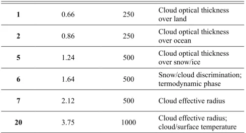
Cloud effective radius and cloud optical depth L2 products are derived using the six visible and near infrared wavelengths (King et al. 1998; Table 2)

Channel Wavelength [µm] Resolution [m] Atmospheric Purpose 1 0.66 250 Cloud optical thickness _{over land}

2 0.86 250 Cloud optical thickness _{over ocean}

5 1.24 500 Cloud optical thickness _{over snow/ice}

6 1.64 500 Snow/cloud discrimination; _{termodynamic phase}

7 2.12 500 Cloud effective radius

20 3.75 1000 Cloud effective radius; _{cloud/surface temperature}

Table 2: spectral characteristics, spatial resolution and principal purposes of cloud bands used in MODIS.