HAL Id: hal-01413813
https://hal.archives-ouvertes.fr/hal-01413813
Submitted on 15 Dec 2016HAL is a multi-disciplinary open access archive for the deposit and dissemination of sci-entific research documents, whether they are pub-lished or not. The documents may come from teaching and research institutions in France or abroad, or from public or private research centers.
L’archive ouverte pluridisciplinaire HAL, est destinée au dépôt et à la diffusion de documents scientifiques de niveau recherche, publiés ou non, émanant des établissements d’enseignement et de recherche français ou étrangers, des laboratoires publics ou privés.
Application of Weighted Empirical Orthogonal Function
Analysis to ship’s datasets
Pascal Terray
To cite this version:
Pascal Terray. Application of Weighted Empirical Orthogonal Function Analysis to ship’s datasets. Quatrième Journée Statistique IPSL (Classification et Analyse Spatiale), Institut Pierre Simon Laplace (IPSL) des Sciences de l’Environnment, 2002, Paris, France. pp.11-28. �hal-01413813�
Application of Weighted Empirical Orthogonal Function Analysis
to ship’s datasets
By Pascal Terray
Laboratoire d’Océanographie Dynamique et de Climatologie, Paris, France
1 . Introduction
Marine ship observations over the vast oceanic regions are crucial to studies of climate variability on timescales from the seasonal to multidecadal. However, any climatic analysis of this historical record is hampered by two difficult problems, namely:
- The systematic instrumental errors which contaminate the ship observations. For example, it is well-known that most of the ship-reports before 1940 contain a large majority of uninsulated bucket Sea Surface Temperature (SST) measurements which are biased low, while the data after the 1940s are mostly injection or insulated bucket SST measurements which are biased high (Bottomley et al., 1990).
- The irregular space-time sampling of the ship-reports. For example, Comprehensive Ocean-Atmosphere Data Set (COADS) summaries provide meteorological variables in the form of monthly means for 2° × 2° latitude-by-longitude cells (Woodruff et al., 1987). In such datasets, the number of observations used to compute a particular monthly mean reflects the number of ships that cross the box that month. Thus, for a particular month, one cell’s mean may be computed from hundreds of observations, while others may be based on only a few, and there may be many cells with missing means due to the poor spatial and temporal coverage outside the main shipping lanes.
The former problem is particularly relevant to studies of multidecadal variability and has led researchers to design instrumental correction procedures for the meteorological and oceanic fields derived from ship-reports and used for assessing climatic changes, e.g. SST and wind.
The latter problem attends almost all climate studies from seasonal to multidecadal timescales, but is particularly relevant to the interannual to multidecadal. The classical solution to cope with this problem is to use some kind of objective analysis. This technique spatially smoothes the oceanic fields by filling the data-void areas with reasonable values which are a linear combination of climatology and anomalies observed in the neighborhood of each grid’s cell. The drawbacks of this solution are: First, the need for a very good climatology which has to be constructed before the analysis. Second, the oceanic fields derived from objective analysis are generally over-smoothed with the undesirable consequence of a decrease in the spatial resolution of the data.
The main objective of this paper is to present a new multivariate statistical method to deal with this last problem. The method may be termed weighted Empirical Orthogonal Function (EOF) analysis or weighted Singular Value Decomposition (SVD) analysis and is a generalization of the traditional EOF analysis, or more precisely, of truncated SVD analysis. This method accounts for the irregular space-time sampling of the ship-reports by the use of weights (a weight is associated with each cell-month entry of the data matrix) in approximating the data matrix by a lower rank matrix in the least squares sense. In contrast, the traditional EOF analysis assumes that all the cells have equal weights in solving the same optimization problem.
Weighted EOF analysis has a long history and has been studied in applied statistics and numerical analysis. In applied statistics, weighted EOF analysis is a particular application of the
Nonlinear Iterative PArtial Least Squares (NIPALS) algorithm introduced by Wold (1966). NIPALS algorithm has been studied by Wold (1966), Wold and Lyttkens (1969) and Gabriel and Zamir (1979). In the context of numerical analysis, weighted EOF analysis is one possible application of separable nonlinear least-squares algorithms. Separable nonlinear least-squares algorithms have been studied extensively, among others, by Golub and Pereyra (1973), Kaufman (1975) and Ruhe and Wedin (1980).
The organization of this paper is as follows: first, the formalism of the weighted EOF analysis is presented and its relationships to traditional EOF analysis are outlined. Second, we illustrate with some examples how weighted EOF analysis is useful for extracting seasonal, interannual and multidecadal climatic signals from ship’s datasets such as COADS summaries. Finally, we highlight the utility of the weighted EOF analysis for different common tasks in meteorology and oceanography.
2 . Theory
The widespread acceptance of EOFs for data reduction purposes, to aid in determining the variability of oceanic and atmospheric fields, or to identify coherent modes of atmospheric parameters suggests that the adaptation of this method to ship’s datasets can provide us an improved tool to extract climatic signals from such noisy data. However, traditional EOF analysis is not well-adapted to ship’s datasets since the method gives the same weight to all the data matrix entries without taking account of the irregular space-time sampling of the ship’s reports when determining eigenvectors and principal components. Moreover, EOFs and principal components are not defined if some data are missing.
By contrast, the new method of analysis we will develop takes directly into account these uncertainties of the data while estimating the EOF model. In order to introduce this new method, it is first useful to review some of the optimal properties of traditional EOFs. This is a necessary step to understand the new method. Principal component or EOF analysis has been derived in a variety of different ways in the meteorological literature, (see, for example the papers by Kutzbach 1967; Jalickee and Hamilton 1977; or Richman 1986). As noted by Horel (1981) or Terray (1995), all these derivations of the method can be shown to be equivalent and differ essentially by the terminology used and the way the results of the analysis are presented. However, among these various methods of derivation, one of them can be readily extended to handle missing values in the data or weights as the others do not.
To demonstrate this, let X denote an p×n data matrix consisting of n time observations (columns
of X) for p grid cells or stations (rows of X ). In the complete case, where X is a full matrix with no missing values, the “full EOF model” can be expressed as a matrix product,
X
=
U.C
where U is an p×p orthogonal matrix (Ut.U=Ip) whose columns are the eigenvectors of the p×psymmetric matrix,
R
=
( )
1X.X
n
t
If the data are centered in rows, R is simply the covariance matrix between the grid’s cells. Furthermore, the elements in the ith row of C represent time variations associated with the ith eigenvector of R (Kutzbach, 1967).
One of the most important optimal properties of EOFs, especially for data reduction purposes, is that maximum inertia of the data matrix is explained by choosing in order the eigenvectors associated with the largest eigenvalues of R. More precisely, it can be shown that the fraction of
the total inertia, Vk, explained by the eigenvectors associated with the k largest eigenvalues can be obtained from Vk l l k l l p n = = =
∑
λ
∑
λ
1 1 min( , )where λ1≥λ2≥ … ≥λl≥… ≥λp≥0 are the eigenvalues of R
In the application of EOFs to highly correlated fields such as those commonly analyzed in meteorology or oceanography, this means that a large portion of inertia can be accounted for by retaining only the first few eigenvectors of R. This leads to define a “restricted k EOF model” to approximate and to study the data. From a geometrical point of view, this restricted k EOF model can be thought as a method of splitting the data matrix X in the following way
€ Xij U Cil E l k lj ij = = +
∑
1In this equation, E is the residual error matrix associated with the restricted k EOF model. In particular, if X is centered in lines, Eij2 can be interpreted as the unexplained (by the restricted k EOF model) residual inertia for the ith station or grid cell and the jth observation.
The optimal properties of EOFs can be stated directly in terms of this restricted k EOF model as follows: the k-component EOF model forms an optimal approximation to the data matrix in the sense of least squares. That is, the minimum of
f
ij il lj l 1 k ij( , )
A B
=
X
−
A.B
=
∑
X
− ∑
A B
= 2 2on all A∈ℜp×k and all B∈ℜk×n is obtained by taking the first k columns of U and the first k rows of C as A and B , respectively. Moreover, this minimum is equal to
2 1
E
=
= +∑
λ
l l k p n min( , )This result is known as the Eckart-Young theorem and it may be derived from the SVD of X (see, for a proof, Gabriel 1978; or Golub and Van Loan 1996).
In this unusual presentation of the EOF technique within the climate community, but not within the statistical one (see, Gabriel 1978), the A and B matrix variables are not constrained to be in some specific formats. It is not necessary for the column vectors of A or the row vectors of B to be pairwise orthogonal and normalized to unity in order to define the k-component model. Indeed, such restrictions on the form of the k-component model are not necessary to adjust this model. Methods for minimizing directly
f ( , )
A B
without computing the eigenvectors of R or the SVD of X are available in the numerical analysis literature (e.g. some variations of the iterative power method, see Golub and Van Loan 1996). In this framework, the normalization used in the traditional EOF analysis appears more as a convenient way to summarize efficiently, in a statistical sense, the results than as a computational need. Moreover, orthonormality constraints on A and B can be relaxed when rotating the EOFs (see Richman 1986) without changing the global form of thek-component model and its descriptive power (e.g. the partition of inertia of X between the product
Now let X be a typical ship’s dataset such as COADS 2°lat × 2°long trimmed monthly means for some area and historical period. In order to take into account the sampling properties of this ship’s dataset while estimating a k-component model, we may correspondingly seek a minimum of
f
ij ij il lj l k ij *A, B
W X
A B
(
)
=
−
=∑
∑
1 2on all A∈ℜp×k and all B∈ℜk×n
Here, W is an p×n positive weight matrix constructed in such a way that the resulting A and B
matrix variables of the k-component model are defined to emphasize the better-observed aspects of the data. In particular, for the extreme case of zero sample size, an entry of the data matrix should play no role in fitting the model; this can be done by assigning zero weights to such cells.
There are several ways to determine this weight matrix in order to take into account that the monthly means for each grid cell are based on samples of widely varying sizes:
a) The simplest method is to set
Wij = 1 if Xij is present Wij = 0 if Xij is missing
This will take care of missing values, but gives the same weight to all non-missing cells in the data matrix.
b) Another choice is to fit the k-component model with weights proportional to size samples Wij = α.Nij
where Nij is the number of ship observations contributing to the cell’s monthly mean Xij. c) A more elaborate strategy is to use some smooth function of the number of observations
Wij = 1 - exp(-Nij / 6)
where again Nij is the number of ship observations used in computing Xij. For this particular weight function, Wij is in the neighborhood of 1 if Nij>10 and near 0.5 if Nij equals 6.
d) Still another strategy for constructing the weight matrix is to use the inverse of the variance or standard error associated with each grid’s cell and month. This information is, for example, available in the distribution files of COADS (Woodruff et al., 1987).
After the weight matrix is constructed, we have to minimize the least-squares problem stated above in order to estimate the k-component model. Note that this cannot be done by solving some eigensystem as in the traditional EOF analysis, and we have to use non-linear least-squares techniques (Gauss-Newton or Marquardt-Levenberg algorithms) to obtain a solution to our problem. The only one restriction we imposed on X for this problem to be solved numerically is that this matrix must have at least one nonmissing element (Wij ≠0) in each line and column. The
algorithms used here to minimize
f
*(
A, B
)
are a generalization of the techniques described in Terray (1995).We first show that the minimization of
f
*(
A, B
)
on all A ∈ℜp×k and all B ∈ℜk×n is a separable nonlinear least-squares problem (Ruhe and Wedin, 1980). This means that the minimization off
*(
A, B
)
is a mixed linear-nonlinear least-squares problem where the associated residual function in ℜp.n is linear in some variables and nonlinear in others. In order to demonstrate this result, we first define V∈ℜp×n, asV
ij=
W
ij . Thenf
ij ij il lj l k ij *A, B
V
X
A B
(
)
=
−
=∑
∑
.(
.
)
1 2=
−
=∑
∑
V X
ij ijV A
ij ilB
lj l k ij(
).
)
1 2Let us now introduce some notations:
- For all α∈ℜm, the symbol diag(α) is used to represent a diagonal m×m matrix with
diagonal elements,
diag(
α
)
jj, equal toα
j.- For any U matrix, the symbol U.j is used to represent the jth column vector of the U matrix. - For any U matrix, the symbol Uj. is used to represent the jth row vector of the U matrix. - For any U matrix, the symbol U+ represents the pseudo-inverse of U (see Golub and Van
Loan, 1996).
- For any U and V matrices, the symbol U#V is used to mean the element by element product of the U and V matrices: [U#V]ij =Uij.Vij .
Now, if we write the matrix V#X as an p.n dimensional vector, we have
f
*( , )
A B
=
e
( , )
A B
2=
e
( , ) ( , )
A B
te
A B
where the residual function e(A,B) in ℜp.n is
€ e diag diag diag j j n n j n ( , ) # . # . # ( ) . ( ) . ( ) . . . . . . . . . . . . . A B V X V X V X V A V A V A B B = − 1 1 1 0 0 0 0 1 0 0 0 0 0 0 0 0 0 0 0 0 0 0 0 0 jj n . . B
In this residual function, we first note that all the lines corresponding to a zero weight (Wij =0) can be eliminated when evaluating this residual function in real computations. The same is true for all the equations of this section. Then,
f
*( , )
A B
= −
y
F
( )
A
b
2 where y j j n n = V X V X V X . . . . . . # . # . # 1 1 , F diag diag diag j n ( ) ( ) . ( ) . ( ) . . . A V A V A V A = 1 0 0 0 0 0 0 0 0 0 0 0 0 0 0 0 0 0 0 0 0 , b j n = B B B .1 . . . .From this formulation of our nonlinear least-squares problem, it is clear that we have a separable minimization problem since for a fixed A matrix we have to solve a linear least-squares problem to determine b. The solution of this linear least-squares problem for a fixed A matrix is
b
=
F
( )
A
+y
More precisely, if we take into account the block structure of F(A), we observe that the best choice of B for a given A matrix is obtained by solving n independent linear least-squares problems and B.j , for j=1,...,n, can be calculated by
B
.j=
[
A
tdiag
(
W A
.j)
]
−1A
tdiag
(
W X
.j)
.j if diag(V.j)A is a regular matrixor
B
.j=
[
diag
(
V A
.j)
]
+(
V
.j#
X
.j)
if diag(V.j)A is a rank deficient matrixInserting now b in
f
*(
A, B
)
, we obtain a new nonlinear functional involving only the A matrixψ
( )
A
= −
y
F
( ) ( )
A
F
A
+y
2=
{
I
p n.−
F
( ) ( )
A
F
A
+}
y
2This modified functional can be termed a variable projection functional since the matrix in braces is an orthogonal projector involving only the A variable (Golub and Pereyra, 1973). Again, if we take into account the block structure of F(A), we obtain an alternative formulation of this nonlinear functional which is more useful for computational purposes
ψ
( )
A
=
{
I
−
[
(
V A
.)
][
(
V A
.)
]
+}
(
V
.#
X
.)
=∑
p j j j j j ndiag
diag
1 2This formulation of our nonlinear least-squares problem shows that the minimization of
f
*(
A, B
)
can be separated in two steps. Once a A matrix has been obtained by minimizing ψ(A), the B matrix can be obtained by solving n independent linear least-squares problems. The rational for employing this separation of variables to minimizef
*(
A, B
)
is given by a theorem proved by Golub and Pereyra (1973). This theorem shows under some differentiability conditionsthat if A is a critical point (or a global minimizer) of ∧ ψ(A), and B∧ is calculated by solving n independent linear least-squares problems as above, then (A∧,B∧) is a critical point (or a global minimizer) of
f
*(
A, B
)
.Methods for minimizing ψ(A) are termed variable projection algorithms and are given by Golub and Pereyra (1973), Kaufman (1975), and Ruhe and Wedin (1980). Their advantages are that they usually solve mixed linear-nonlinear least-squares problems like
f
*(
A, B
)
in less time and fewer function evaluations than standard nonlinear least-squares codes, and that no starting estimate of the linear variable B is required. In the context of weighted EOF analysis, they offer also other advantages as we will see below. Our implementation codes are more akin to the Gauss-Newton algorithms of Ruhe and Wedin (1980) with some important adaptations due to space memory limitations and for taking advantage of the sparse and structured derivatives of the functional ψ(A) to reduce the CPU time. For more details about the difficult numerical problem involved, the reader is referred to the above publications.Now let us consider in some details how to compute the derivative of
f
*(
A, B
)
efficiently. It is also possible to compute the derivative of ψ(A) (Golub and Pereyra, 1973; Ruhe and Wedin, 1980), however in our application this derivative is not used directly and its computational cost is much higher. We first state some well-known results:Suppose that we have a (non)linear least-squares problem
ϕ
( )
x
=
e x
( )
2=
e x e x
( ) ( )
tThe derivative of the object function ϕ is
ϕ
' ( )
x
=
2
e x e x
' ( ) ( )
twhere ϕ’ and e’ are the derivatives of ϕ and e, respectively. Now, if the residual function e is of the form
e x
( )
= −
y
F x
( )
where y∈ℜq is a constant vector and F a function of x∈ℜm. We have
€
e x
' ( )
= −
F x
' ( )
where F’(x) is the q×m matrix of partial derivatives of F and€
where ϕ’(x) is a m dimensional vector and is simply the gradient of ϕ. In the simple case of a linear least-squares problem, we have
€
F x
( )
=
G
x
and€
e x
' ( )
= −
G
where G is a q×m matrix and the derivative of ϕ is simply
ϕ
' ( )
x
=
2 G G
[
tx
−
G
ty
]
Now, we have
f
*( , )
A B
=
e
( , )
A B
2= −
y
F
( )
A
b
2and the matrix of derivatives of the residual functione(A,B) with respect to b is simply –F(A) and
is very sparse with only k elements in each row. Finally, the derivative of
f
*(
A, B
)
with respect to b is easy to compute with the above results∂
∂
f
b
F
F
b
F
y
t t *( , )
( )
( )
( )
A B
A
A
A
=
2
[
−
]
For computing the derivative of
f
*(
A, B
)
with respect to A, we first note that the role of A and B inf
*(
A, B
)
are interchangeable. Consequently both A and B occur linearly inf
*(
A, B
)
and this functional may also be written as follows:f
*( , )
A B
= −
z
G
( )
B
a
2 where z t i i t p p t =(
)
(
)
(
)
V X V X V X 1. 1. . . . . # . # . # , G diag diag diag t i t p t ( ) ( ) . ( ) . ( ) . . . B V B V B V B = 1 0 0 0 0 0 0 0 0 0 0 0 0 0 0 0 0 0 0 0 0 , a t i t p t =( )
( )
( )
A A A 1. . . . .Now the derivative of
f
*(
A, B
)
with respect to a is also easy to compute∂
∂
f
a
G
G
a
G
z
t t *( , )
( )
( )
( )
A B
B
B
B
=
2
[
−
]
In any of the weighted EOF analyses presented in this paper the Euclidean norm of the gradient of
f
*(
A, B
)
has been reduced by many orders of magnitude, thereby suggesting that at least a local minimum of the functionalf
*(
A, B
)
has been obtained in each case.After the nonlinear least-squares problem, minimizing
f
*(
A, B
)
, is solved, it is an easy task to obtain suitable orthonormalization of the A and B matrices of the weighted k-component model similar to the traditional ones in the restricted k EOF model by computing the SVD of the A . B product. Note that there is no need to compute the A.B product in this final computation since the SVD of this product can be easily deduced from the two smallest SVD of A and B , respectively. LetA.B
=
U
ˆ ˆ ˆ
kΣ
kV
ktbe the SVD of A.B. Where
ˆ
U
kis the matrix formed by the first k eigenvectors of (AB).(AB)t stored columnwise;ˆ
V
k is the matrix formed by the first k eigenvectors of (AB)t.( AB) stored columnwise;ˆ
Σ
k is a k×k diagonal matrix whose diagonal elements are the singular values, e.g. the square roots of the first k eigenvalues of (AB).(AB)t and (AB)t.( AB) arranged in decreasing order.Note that this SVD has no more than k terms with a singular value distinct from zero since A . B is of rank ≤k. With these notations, the first k “principal components” of the weighted EOF
analysis are just
€
ˆ ˆ
Σ
kV
ktand the first k “eigenvectors” may be defined as
U
ˆ
k if the lines and columns of X referred to stations and time observations, respectively.Finally, to get some estimate of the percentage of inertia explained by each principal component of the weighted EOF model from the singular values, µq, of the A.B product, we can compute the statistics Iq q n ij ij j n ij j n i p =
( )
= = =∑
∑
∑
µ2 2 1 1 1 W X W for 1<=q<=kThe numerator in the right hand side of this equation represents the variance of the qth estimated principal component, while the denominator is the sum of the weighted variance of the p variables. The mutual consistency of these k individual statistical estimates can be checked with the following statistic
€
I
tot=
V AB
#
2/
V X
#
2This last ratio gives the true percentage of the weighted inertia of X explained by the k-component model in the weighted EOF analysis. This important geometrical property holds since it is readily observed that we have the equalities
€
2 2 2
V
.j#
X
.j=
V
.j#
AB
.j+
V
.j#
(
X
.j-
AB
.j)
for j=1 to nwhen a separable nonlinear least-squares algorithm is used to minimize
f
*(
A, B
)
. By summing all these equalities for j=1 to n, we obtain€
2 2 2
V X
#
=
V AB
#
+
V
#
(
X AB
-
)
The left-hand side of this equation is the weighted inertia of X, while the first term in the right-hand side is the weighted inertia of X explained by the k-component model. Consequently, Itot gives the true fraction of the weighted inertia of X described by the weighted EOF analysis with k components.
3 . Examples
In order to illustrate the application of this technique and to show that this method allows us to analyze the natural variability exhibited by data of varying reliability, two classical ship’s datasets were analyzed using the weighted EOF technique.
a. Example 1
The first example is a weighted EOF analysis of the January 1993 version of the Global Ocean Surface Temperature Atlas (GOSTA, Bottomley et al., 1990). The data in this atlas are presented as monthly anomalies on a 5° latitude × 5° longitude grid wherever data existed. The data were extracted for the period from 1900 to 1991. The weight function used in this analysis is simply: Wij = 1 if Xij is present and Wij = 0 if Xij is missing. Note that this is not a very good choice since this will give the same weight to all non-missing data, but there is no information on the number of ship-reports used to compute monthly anomalies for individual grid cells in the distribution files of GOSTA.
-3 -2 -1 0 1 2 Years Amplitude (C) 1900 1910 1920 1930 1940 1950 1960 1970 1980 1990
With this weight function, a two-components model was estimated. At the end of the iterations, the two-components model explains a little less than 16% of the total weighted inertia of the data. Note that the norm of the gradient of the objective function has been decreased by several orders of magnitude from the initialization to the end of the algorithm.
The first estimated principal component is showed in Figure 1. This time series as presented has unit variance. The associated eigenvector is shown in Figure 2. This eigenvector has been multiplied by the square root of its associated eigenvalue. In this way, the spatial loadings depicted in Figure 2 can be interpreted as covariance coefficients between the grid’s cells and the time series plotted in Figure 1.
Interdecadal changes of SST are particularly evident in this first principal component. The time series suggests a cold start of the twentieth century with a sudden warming between about 1920 and 1940. After World War II, the time series suggests a slight cooling until 1976. After this date, a slow but regular warming took place. Indeed, this first estimated principal component is very similar to the time series of global and hemispheric temperature anomalies presented by Parker et al. (1994). However, an important discrepancy between our time component and the estimates of Parker et al. (1994) is that recent decades are not substantially warmer than the preceding ones on Figure 1. Note also that the first part of this time series is much more noisy than the last part; this may be due to our choice of the weight function since we gave the same weight to all data entries with non-missing values in the atlas without taking account of the number of ship-reports used to construct the anomalies. In the same fashion, the strongly negative time coefficients during World War II are due to high and isolated positive monthly anomalies in the central and eastern Pacific which were likely computed using very few ship observations. We hypothesize that a much better job can be done about these two problems if we use a more appropriate weight function.
0.25 0.50 -0.50 0.00 0.25 0.50 -0.25 0.25 0.00 0.50 0.75 0.25 0.50 0.25 0.00 0.00 -0.25
135E 180 135W 90W 45W 0 45E 90E
90S 60S 30S 0 30N 60N 90N -1.00 -0.50 0.00 0.50 1.00 1.50 COVARIANCE
Figure 2: GOSTA global SST estimated EOF1 (10.6%, rank=2).
The spatial pattern associated with this time series suggests that these decadal SST variations are well-marked in the midlatitude North Pacific and in parts of the middle-to high-latitude Southern Ocean (Figure 2). By contrast, the areas in the central and eastern equatorial Pacific and also in the South Indian Ocean are negatively correlated to this time series. It may be pointed that this fact is
also evident in the global fields of decadal annual surface temperature anomalies presented by Parker et al. (1994).
The second estimated principal component is shown in Figure 3. A strong interannual signal seems to be present in this time series with a time-scale of about 3 to 4 years, especially in recent decades. A sudden warming may also be noticed after 1976. The estimates during World War II are again unreliable. -3 -2 -1 0 1 2 3 4 Years Amplitude (C) 1900 1910 1920 1930 1940 1950 1960 1970 1980 1990
Figure 3: GOSTA global SST weighted EOF analysis (rank=2). Estimated SST EOF2 amplitude.
0.25 0.25 0.00 0.25 0.25 0.00 0.500.25 -0.25 0.00 0.25 0.75 0.75 0.50 0.25 -0.25 0.00
135E 180 135W 90W 45W 0 45E 90E 90S 60S 30S 0 30N 60N 90N -1.00 -0.50 0.00 0.50 1.00 COVARIANCE
The spatial loadings associated with this time series exhibit the well-known ENSO signature with a warm tongue in the central and eastern Pacific, and with smaller amplitudes and opposite phase in the middle latitude North and South Pacific (Figure 4). Some positive areas also are noticeable in the Indian Ocean. Thus, this second principal component and its associated spatial pattern suggest that recent warmings may have some connections with ENSO and a sudden change of the climate mean state which took place in the pacific regions during 1976.
b. Example 2
The second example is taken from the COADS trimmed monthly mean summaries (Woodruff et al. 1987). SSTs over the Indian Ocean (41°S-31°N and 29°-121°E) were extracted for the period 1900 to 1992. Note that these data are not anomalies but estimates of monthly mean SST on a 2° latitude × 2° longitude grid.
The weight matrix used in this analysis was constructed with the smooth function of the number of observations contributing to each cell’s monthly mean value discussed in Section 2. Again, a two-component model was estimated from the data by the weighted EOF technique. These two components explain more than 99.8% of the total weighted inertia.
The first principal component is, to a very good approximation, sinusoidal with an annual period (Figure 5). An interdecadal trend seems also to be present in this time series with a sudden warming after 1976. The same results may be obtained by averaging the data for the whole Indian Ocean (Terray, 1994). The associated spatial pattern exhibits a north to south gradient of SST (Figure 6). Note also that SST is colder off the African coast.
0.90 0.95 1.00 1.05 1.10 Years Amplitude (C)
Figure 5: COADS Indian Ocean SST weighted EOF analysis (rank=2). Estimated SST EOF1 amplitude.
2 8 26 14 16 18 20 22 24 26 26 28
40E 60E 80E 100E 120E
30S 10S 0 10N 30N 10.00 15.00 20.00 25.00 30.00 SST AMPLITUDE (°C)
Figure 6: Indian Ocean SST estimated EOF1 (98.6%, rank=2).
The second principal component (Figure 7) is still marked by an annual period but its spatial pattern (Figure 8) shows a characteristic phase difference between North and South which adds an annual modulation to the first principal component and its associated eigenvector.
-2 -1 0 1 2 Years Amplitude (C)
Figure 7: COADS Indian Ocean SST weighted EOF analysis (rank=2). Estimated SST EOF2 amplitude.
0 . 5 2.0 1.5 2.0 1.5 2.0 1.5 1.0 0.5 1.0 0.0 -1.0 -1.5 -2.0 -1.5 -1.0 -0.5 0 . 5 0.0
40E 60E 80E 100E 120E 30S 10S 0 10N 30N -5.00 0.00 5.00 10.00 SST AMPLITUDE (°C)
Figure 8: Indian Ocean SST estimated EOF2 (1%, rank=2).
In order to present in a more traditional manner the annual signal described by these two time series and their associated spatial loadings, a climatology of Indian Ocean SSTs was computed from the rank 2 weighted approximation of the data given by the two-component model. This climatology may then be compared to a traditional climatology obtained from an objective analysis in order to show the coherence of the results.
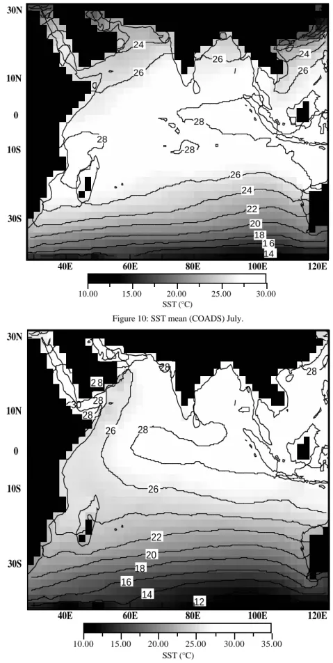
The mean SST fields for January and July obtained from the rank 2 weighted approximation of the data are shown in Figures 9 and 10.
SST patterns in the January mean field are dominated by highest temperatures (28°C) in the eastern Indian Ocean between the equator and about 15°S and also near Madagascar. Strong SST gradients are evident over the higher latitudes of the southern Indian Ocean.
The July mean SST fields show the effect of upwelling and monsoon cooling near the African coast associated with the Somali jet and to the south of Peninsular India while other parts of the North Indian Ocean are still dominated by warmer SST. All these patterns are found in classical atlases (Hastenrath and Lamb, 1979; Bottomley et al., 1990).
1 6 24 26 26 24 26 28 28 28 26 24 22 20 18 14
40E 60E 80E 100E 120E 30S 10S 0 10N 30N 10.00 15.00 20.00 25.00 30.00 SST (°C)
Figure 9: SST mean (COADS) January.
2 8 12 14 30 28 28 28 16 18 20 22 26 26 28 28
40E 60E 80E 100E 120E
30S 10S 0 10N 30N 10.00 15.00 20.00 25.00 30.00 35.00 SST (°C)
4 . Conclusions
EOF analysis has been widely used to explore the spatial and temporal relationships within large geophysical datasets. This success can be explained by the ability of EOFs to compress the main modes of variability in the original dataset into a few time series and associated spatial patterns. Indeed, the EOF technique can be thought of mathematically as a method for approximating data matrices by matrices of lower rank since conventional EOFs provide the best approximation of a data matrix in the sense of least-squares under the assumption that all the data entries have the same weight equal to one.
This paper presents an extension of conventional EOFs when weights are assigned to data entries in the original dataset. The new method which may be termed weighted EOF analysis is designed to fit a lower rank least-squares approximation to a data matrix with a general choice of positive weights. If the weight matrix is carefully constructed, this new tool allows us to analyze the natural variability exhibited by data of varying reliability. It must also be emphasized that the proposed method directly takes care of missing values by assigning zero weights to such data entries.
Indeed, there are many situations in which weighted EOF analysis is more appropriate than conventional EOFs. In particular, weighted EOF analysis is shown to be a useful tool for extracting climatic signals from ship’s datasets which are characterized by a strong irregular space-time sampling.
In the context of ship datasets with irregular space-time sampling, weighted EOF analysis can be particularly useful for the following purposes:
- accurate and robust detection of climate signals (annual, interannual and multidecadal) on a grid-mesh, directly from the ship observations;
- blended analysis of marine and land datasets; - interpolation of missing values;
- derivation of climatologies and smooth oceanic fields;
- sensitivity experiments (e.g. by using various weight matrices with the same dataset).
With this new technique, it is also possible to design robust versions of many multivariate analysis procedures used for climate studies, including:
- Principal Component Analysis (PCA);
- Singular Spectrum Analysis (SSA) and Multi-channel Singular Spectrum Analysis (MSSA); - Canonical Correlation Analysis (CCA);
- Singular Value Decomposition Analysis (SVD).
Finally, it is possible to derive powerful nonlinear statistical prediction algorithms from weighted EOF analysis as well as new algorithms for estimating missing values. These other applications of weighted EOF analysis will be reported in detail elsewhere.
References
Bottomley, M., C.K. Folland, J. Hsiung, R.E. Newell, and D.E. Parker, 1990: Global ocean
surface temperature atlas "GOSTA". Joint project of the UK Meteorological Office and
Gabriel, K.R.,and S. Zamir, 1979: Lower rank approximation of matrices by least squares with any choice of weights. Technometrics, 21, 489-498.
Gabriel, K.R., 1978: Least squares approximation of matrices by additive and multiplicative models. J. Roy. Statist. Soc., B, 40, 186-196.
Golub, G.H., and V. Pereyra, 1973: The differentiation of pseudo-inverses and non-linear least squares problems whose variables separate. SIAM J. Num. Anal., 10, 413-432.
Golub, G.H., and C.F. Van Loan, 1996: Matrix Computations. 3d ed. Johns Hopkins University Press, 642 pp.
Hastenrath, S., and P.J. Lamb, 1979: Climatic atlas of the Indian Ocean. Part I: Surface climate
and atmospheric circulation. The University of Wisconsin Press, Madison, 109 pp.
Horel, J.D., 1981: A rotated principal component analysis of the interannual variability of the Northern Hemisphere 500mb height field. Mon. Wea. Rev., 109, 2080-2092.
Jalickee, J.B., and D.R. Hamilton, 1977: Objective analysis and classification of oceanographic data. Tellus, 29, 545-560.
Kaufman, L., 1975: Variable projection method for solving separable nonlinear least squares problems. BIT, 15, 49-57.
Kutzbach, J.E., 1967: Empirical eigenvectors of sea level pressure, surface temperature, and precipitation complexes over North America. Journal of Applied Meteorology, 6, 791-802. Parker, D.E., P.D. Jones, C.K. Folland, and A. Bevan, 1994: Interdecadal changes of surface
temperature since the late nineteenth century. J. Geophys. Res., 99 (D7), 14,373-14,399. Richman, M.B., 1986: Review article, rotation of principal components. J. Climatol., 6, 293-335. Ruhe, A., and P. A. Wedin, 1980: Algorithms for separable nonlinear least squares problems.
SIAM Review, 22, 318-337.
Terray, P., 1994: An evaluation of climatological data in the Indian Ocean area. J. Meteor. Soc.
Japan, 72, 359-386.
Terray, P., 1995: Space/Time structure of monsoons interannual variability. J. Climate, 8, 2595-2619.
Wold, H., and E. Lyttkens, 1969: Nonlinear iterative partial least squares (NIPALS) estimation procedures. Bull. Inter. Statist. Inst., 43, 29-51.
Wold, H., 1966: Nonlinear estimation by iterative least squares procedures. Research Papers in
Statistics, F.N. David ed., Wiley, pp. 411-444.
Woodruff, S.D., R.J. Slutz, R.L. Jenne, and P.M. Steurer, 1987: A Comprehensive Ocean-Atmosphere Data Set. Bull. Amer. Meteor. Soc., 68, 1239-1250.