BeatDB v3 : a framework for the creation of predictive datasets from physiological signals

(1)

BeatDB v3: A Framework for the Creation of

Predictive Datasets from Physiological Signals

by

Steven Anthony Rivera

S.B., Massachusetts Institute of Technology (2016)

Submitted to the Department of Electrical Engineering

and Computer Science

in partial fulfillment of the requirements for the degree of

Master of Engineering in Computer Science and Engineering

at the

MASSACHUSETTS INSTITUTE OF TECHNOLOGY

June 2017

c

○ Massachusetts Institute of Technology 2017. All rights reserved.

Author . . . .

Department of Electrical Engineering

and Computer Science

May 26, 2017

Certified by . . . .

Una-May O’Reilly

Principal Research Scientist

Thesis Supervisor

Certified by . . . .

Erik Hemberg

Research Scientist

Thesis Supervisor

Accepted by . . . .

Christopher J. Terman

Chairman, Masters of Engineering Thesis Committee

(2)

(3)

BeatDB v3: A Framework for the Creation of Predictive

Datasets from Physiological Signals

by

Steven Anthony Rivera

Submitted to the Department of Electrical Engineering and Computer Science on May 26, 2017, in partial fulfillment of the

requirements for the degree of

Master of Engineering in Computer Science and Engineering

Abstract

BeatDB is a framework for fast processing and analysis of physiological data, such as arterial blood pressure (ABP) or electrocardiograms (ECG). BeatDB takes such data as input and processes it for machine learning analytics in multiple stages. It offers both beat and onset detection, feature extraction for beats and groups of beats over one or more signal channels and over the time domain, and an extraction step focused on finding condition windows and aggregate features within them.

BeatDB has gone through multiple iterations, with its initial version running as a collection of single-use MATLAB and Python scripts run on VM instances in Open-Stack and its second version (known as PhysioMiner) acting as a cohesive and modular cloud system on Amazon Web Services in Java. The goal of this project is primarily to modify BeatDB to support multi-channel waveform data like EEG and accelerom-eter data and to make the project more flexible to modification by researchers. Major software development tasks included rewriting condition detection to find windows in valid beat groups only, refactoring and writing new code to extract features and prepare training data for multi-channel signals, and fully redesigning and reimple-menting BeatDB within Python, focusing on optimization and simplicity based on probable use cases of BeatDB. BeatDB v3 has become more accurate in the datasets it generates, usable for both developer and non-developer users, and efficient in both performance and design than previous iterations, achieving an average AUROC in-crease of over 4% when comparing specific iterations.

Thesis Supervisor: Una-May O’Reilly Title: Principal Research Scientist Thesis Supervisor: Erik Hemberg Title: Research Scientist

(4)

(5)

Acknowledgments

I could not have completed my thesis or work on BeatDB without the help of numerous individuals and groups along the way.

I’d like to thank Una-May O’Reilly for her kindness and direction throughout the development of this project. She made this process very bearable, meaningful, and fun, and I am very grateful to have a mentor as intelligent, insightful, and personable as her.

I’d also like to thank Erik Hemberg for preparing me for this thesis over Summer 2016 by coaching me through further development of the MLBlocks platform. He also provided very valuable advice and direction for the redesign of BeatDB and without him, I’m not sure that BeatDB would have come out as optimized and elegant as it did.

I’d like to thank Alejandro Baldominos for helping me understand how PhysioMiner worked and providing a groundwork for BeatDB v3 by developing the preprocessing module. Without Alejandro’s help, I would have taken significantly more time to understand how this project worked and would not have been able to accomplish as much as I ended up doing.

I’d like to thank my mother, Claudia Rivera, grandmother, Maria Rosales, and aunt, Cecilia Rosales, for their constant support throughout my academic career and the sacrifices they made to ensure that I had these amazing opportunities available to me.

I’d like to thank Gabriela Carrillo for always being there for me every step of the way and believing in me even when I didn’t believe in myself.

I’d like to thank Juan Huertas, Jordan Smith, and Reymundo Cano for giving me plenty of opportunities to destress and have fun when work became overwhelming.

(6)

I’d like to thank my band, Love and a Sandwich, for allowing me to continue pursuing my passion for drumming throughout my undergrad and graduate years of study.

Lastly, I’d like to thank my fraternity, Theta Delta Chi, for providing me with a nurturing, supportive, and academic environment over the entirety of my education at MIT.

(7)

List of Figures

3-1 Group Window Diagram . . . 36

3-2 BeatDB v0 System Overview . . . 37

3-3 BeatDB v1 System Overview . . . 39

3-4 Valid Beat Group Diagram . . . 43

3-5 PhysioMiner System Overview . . . 50

(12)

(13)

List of Tables

3.1 BeatDB v1 and PhysioMiner Comparison. . . 46

3.2 PhysioMiner (original) and PhysioMiner (VBG) Comparison . . . 49

5.1 Experimentation Parameters . . . 71

5.2 PhysioMiner and BeatDB v3 Version Comparisons. . . 72

5.3 High Level Comparison of All BeatDB Iterations. . . 77

(14)

(15)

Chapter 1 Introduction

BeatDB is a project developed and maintained by the Anyscale Learning for All group (ALFA) in the Computer Science and Artificial Intelligence Laboratory (CSAIL) at MIT. It is a framework that allows users to input both single and multi-channel physiological data and analyze patterns and correlations within the data. It does this by parsing waveforms into individual chunks (such as beats, if the waveform can be expressed in them) while extracting additional features from each chunk in the population/extraction stage. Afterward, BeatDB uses this information, along with aggregated features over groups of chunks, to form a machine learning dataset in the condition detection/aggregation stage.

Normally when researchers want to conduct an experiment using physiological data, they need to spend time figuring out how to parse the data from the raw waveform. Given the variability in the way that data can be stored, this process tends to be specific to the type of data that the researchers have. Once the data has been parsed into a more readable and malleable form, the researchers need to develop a pipeline to process the data, usually making the pipeline very specific to the format of the parsed data. While this tends to lead to output that is very close to what the researchers want, the software they develop for these experiments is not typically reusable since it is so specific to the data and the way that the researchers processed it along the pipeline. Given the complexity of this process, it can take some amount of time and

(16)

use of resources to develop.

Why should researchers use BeatDB? BeatDB allows researchers and scientists to cut down on time needed for prediction studies and data processing without sacrificing any of the parameterization and specificity to the data possible with custom (and often single-use and unrefined) scripts. With BeatDB v3, users are given freedom to define their own features, validity functions, and input signal types (such as ambulatory blood pressure (ABP)) within the framework. They are also able to easily integrate any cloud based service within the framework, with Amazon Web Services (AWS) and local modes supported by default. Additionally, BeatDB v3 improves upon many issues and design concepts found in previous iterations of BeatDB, as seen in the comparison table 5.3 and expanded upon in section 5.2.

1.1 Development Background

BeatDB has gone through multiple iterations, with its key ideas having been previ-ously implemented in three different languages and for two different instance frame-works (including a local mode, limited to a single worker and smaller test datasets). BeatDB v0, mentioned in detail in Waldin’s thesis, was not a full system but a col-lection of single-use MATLAB and Python scripts used for both beat onset detection and the extraction of additional features from every detected beat. This iteration served as a prototype for the population/extraction stage of the next iteration of BeatDB.

BeatDB v1, which was a complete attempt at creating a distributed system for beat detection and feature extraction, condition detection, and feature aggregation, was the first attempt at making BeatDB a fully fledged application. Computation was run on a network of OpenStack instances at CSAIL, but as this was hard-coded into the framework, it prevented BeatDB from being accessible to many audiences. Addition-ally, BeatDB v1’s design focus was on functionality, not general usability, rendering customization of the platform difficult. This iteration of BeatDB did not provide

(17)

features that would be expected of a user-based system and was difficult to adapt for use cases other than the ABP use case demonstrated in Dernoncourt’s thesis on BeatDB.[7]

PhysioMiner, known as BeatDB v2, reworked the scripts that comprised BeatDB v1 into a modular and cohesive cloud based system hosted on Amazon Web Services (AWS). The algorithms in the scripts were rewritten in Java, with Python used for user-defined feature, condition, and aggregation functions.[10] At the time of develop-ment, AWS and the interest in cloud technologies was relatively new. Given this, and the need for a user-based version of BeatDB, ALFA implemented PhysioMiner on top of AWS. The scripts for the "analytics sub-framework" were the direct inspiration for PhysioMiner, with the four steps outlined in the hypothesis testing framework section of the NIPS workshop paper[8] becoming the four major stages of the PhysioMiner system.[8]

Since its development in 2014, PhysioMiner remained in use in ALFA group until De-cember 2016 after a large processing job unveiled multiple issues with the framework and its scalability potential, leading to numerous message timeouts, delayed process-ing time for each message, and a significant amount of money beprocess-ing spent on the computation (one specific computation over the entire MIMIC-II ABP dataset cost over $1500 dollars). Although PhysioMiner was built with the BeatDB v1 design in mind, its design was too over-engineered and intertwined with AWS, limiting its effec-tiveness for large tasks. Feature creep and poor design choices caused PhysioMiner to bloat over years of maintenance, making it more and more difficult for new researchers to use the platform. Issues with the AWS framework, primarily those caused by mes-sage timeouts in the queues, drastically affected computation time and cost. The issues stemming from this large computation forced ALFA to reevaluate PhysioMiner and compare its implementation with the BeatDB v1 design.

After evaluation, multiple objectives were created for a new iteration of BeatDB, fo-cusing on usability, efficiency, and correctness, along with the implementation of new

(18)

features that allow for more complex generation of feature data from beats. This iteration of BeatDB, called BeatDB v3, and the design and implementation of this new iteration, are the focus of this thesis.

1.2 Objectives

There are a number of research questions for this body of work, most of them related to the creation of BeatDB v3. These are listed and discussed below.

Does the PhysioMiner system achieve comparable correctness to the BeatDB v1 sys-tem?

Given the differences in system design and implementation, the best way to com-pare PhysioMiner to BeatDB v1 is to comcom-pare the results of specific computations on both systems. The process of verifying the correctness of the PhysioMiner software will allow us to determine how similar results of learning on generated datasets from PhysioMiner’s implementation are to BeatDB v1’s design, and as a result, will guide our decisions regarding the design and implementation of BeatDB v3.

How can the BeatDB system be more usable?

Though each subsequent iteration of BeatDB has attempted to make the software easier to use for non-developers, there is still more progress to be made in simplifying the method of control over the parameters that the user has. The process of running the PhysioMiner software, both locally and on the cloud, can be confusing, even for advanced users. New iterations of BeatDB should be designed with a focus on the technical ability of expected users, but not to the point that functionality and effi-ciency are hindered. Additionally, the source code of the software should be clear and understandable for developers who wish to modify the source code so that the system stays efficient over time and the inevitable maintenance it will be put through.

(19)

How can the BeatDB system be more efficient, in terms of performance, software de-sign, and implementation?

PhysioMiner became bloated over multiple years of use and modification and, as a result, started to deviate from its original design. After performing a code analysis of PhysioMiner, we discovered multiple ingrained issues with the implementation that have a large negative effect on computation run-time. When processing data, Phys-ioMiner does not strive for efficiency, requiring multiple full passes over file data for a single population task. Additionally, the process for importing feature functions is inefficient, forcing PhysioMiner to wait for file I/O for every feature calculation and requiring that each feature script be redownloaded from S3 for every function call related to that feature.

Given the complexity of the PhysioMiner system and how rigid various parts of the design are, attempting to fix PhysioMiner’s low-level implementation issues would re-quire many resources and would ultimately lead to a weaker system, especially when considering the amount of patching that would need to be done to add functionality and increase efficiency in the software. Rather than fix PhysioMiner and add more bloat to the source code, ALFA group decided that rewriting BeatDB in Python will allow for the simplification of various parts of the system design.

Coding in Python makes it easier to add new software features to the system, and having the hindsight of what issues arose in BeatDB v2 allows for revision of system design mistakes made in the past. Performance-wise, coding in Python will heavily reduce the number of subprocess calls made for the user-defined scripts necessary for certain steps. Additionally, coding in Python will greatly speed up the system as processes will no longer need to wait for the costly file I/O overhead for each feature function’s results.

Does the BeatDB v3 system achieve comparable correctness to the PhysioMiner and BeatDB v1 systems?

(20)

Because BeatDB is being reimplemented based on previous designs, it needs to be reevaluated for correctness and consistency with previous iterations to ensure that similar results are generated at each newly developed stage and that the new BeatDB software is performing as expected. Executing correctness tests, similar to those used to compare PhysioMiner and BeatDB v1 at the beginning of this work, will give con-fidence in the consistency of BeatDB v3’s results with those from previous systems.

How can functionality be added to BeatDB v3 to allow for more customization, input filtering, and the ability to process multi-dimensional waveforms?

Though this thesis has been focused on the creation of the BeatDB v3 system, its initial objective was to add support for multi-channel features and multi-dimensional waveforms to PhysioMiner. Discovery of the issues with PhysioMiner led to a focus on a new iteration of BeatDB, but multi-dimensional waveform support remains a priority in the development of BeatDB v3. The design of BeatDB v3 made it simple to adapt the codebase for multi-dimensional waveforms and multi-channel features, allowing users to define their own multi-dimensional signal types and multi-channel features without much more complexity than is already required for customized single-channel signal types and features.

BeatDB v3 also includes standalone features related to the filtering of input file sizes and preprocessing of input data to allow the user to have greater control over their computations. Following its design goals, BeatDB v3 is more user-friendly, only re-quiring a configuration file to parse all arguments for all steps at once in order to simplify the execution of the system. Lastly, users will be able to add support for cloud frameworks of their choice, allowing BeatDB to be run on frameworks other than AWS.

(21)

1.3 Organization

∙ Chapter 2 presents the architecture of the BeatDB design and its realization in previous iterations of the system

∙ Chapter 3 discusses PhysioMiner in detail, focusing on output comparisons with findings from Waldin’s thesis and modifications made to the system

∙ Chapter 4 provides motivation for and details the design of BeatDB v3

∙ Chapter 5 details the testing and demonstration of BeatDB v3 with original ABP data used in previous iterations of BeatDB

∙ Chapter 6 concludes this thesis and discusses future work and goals for the BeatDB v3 platform

∙ Appendix A contains technical information and specifics regarding the imple-mentation and usage of BeatDB v3

∙ Appendix B contains pseudocode for specific algorithms that are critical to BeatDB v3

(22)

(23)

Chapter 2 Background

2.1 Related Work

Despite research into similar frameworks, it seems that BeatDB is one of the few frameworks that combines several of the specific concepts behind it, such as onset detection, feature aggregation, and the ease of customization coupled with its user-based design. BeatDB is a novel system primarily because of its focus on flexibility toward multiple signal types and the combination of its provided features, such as the coupling of beat detection along with condition detection and window aggregation. Despite this, there is a large amount of work related to different parts of BeatDB, as feature extraction of signal data and prediction of medical events are large fields of interest in computing, among other components of BeatDB.

2.1.1 Feature Engineering

Feature engineering is a popular subject for research because features impact model prediction accuracy, meaning that findings can have a large impact on future ma-chine learning research.[19] Because many of the signal types are waveforms, using wavelets, particularly wavelet transforms, is a common approach for feature engineer-ing and extraction research. In fact, wavelets have been shown to outperform the fast Fourier transform as a spectral analysis tool for detecting brain diseases.[1] A paper

(24)

from 1997 describes the use of artificial neural networks along with the wavelet trans-form to classify EEG signals between normal, schizophrenic, and obsessive-compulsive classes.[12] One group of researchers uses the stationary wavelet transform on EEG data to"reduce artifacts from scalp EEG recordings to facilitate seizure diagnosis/de-tection for epilepsy patients."[5] In the hardware realm, researchers have designed a wavelet-based ECG detector for use in implantable pacemakers, noting that "wavelet-based detection algorithms [are] generally considered as one of the most effective algorithms."[19]

Despite this, there is still value in researching other features. An algorithm proposed in 2013 uses local extreme values and their dependencies to extract locations of ECG deflections, allowing the algorithm to form the beat and detect anomalies in real-time.[29] Another group of researchers proposed a method for monitoring cerebral autoregulation in patients that focuses on an improvement to the signal abnormality index algorithm described in the ABP section above. By adding two simple summa-tion features, the researchers were able to greatly improve the specificity of the signal abnormality index for ABP data.[35]

Feature extraction can also be automated via usage of deep belief networks, as shown in the following examples. A group of researchers used this approach to predict emotions by "automatically [extracting] features from raw physiological data of 4 channels in an unsupervised fashion and then [building] 3 classifiers to predict the levels of arousal, valance, and liking based on the learned features."[32] This imple-mentation of deep belief networks is unique because it is the first attempt at using them to predict emotions, but deep belief networks have been used frequently with physiological data in the past, showing utility in both handwriting recognition[15] and classifying between stages in a sleep cycle[14], among other applications.

(25)

2.1.2 Prediction of Medical Events

The prediction of medical events is a popular field of research as it has various appli-cations in the real world. A medical event is one of interest that usually denotes some sort of issue with a patient, such as an acute hypotensive episode or hemodynamic in-stability. Researchers at MIT used symbolic analysis and clustering of cardiovascular signals, available via ECG data, to predict "unexpected events" of interest.[28] The researchers used morphological features to partition beats into classes that could be represented by symbolic strings "corresponding to the sequence of labels assigned to the underlying unit." Afterward, they searched "for significant patterns in the reduced representation resulting from symbolization," allowing them to quickly analyze the data for irregularity with the idea that "[symbol] variations that are unlikely to occur purely by chance" are likely to be the most medically relevant.[28] The researchers had success with their techniques, uncovering multiple examples of heartbeat irregu-larities while achieving very high consistency with cardiologist opinion.

Additional research has been conducted to attempt to predict more specific cardio-vascular events. Two researchers at the Bhoj Reddy Engineering College for Women have developed an algorithm for detecting arrhythmia from ECG signals using ST seg-ment and QRS detection. Once these regions have been detected, signal extraction occurs by using a combination of discrete wavelet transformation and support vector machine techniques to uncover ECG features and classify each beat as arrhythmic or normal.[23] Similarly, research conducted at the Khulna University of Engineering & Technology also used support vector machines to detect cardiac diseases such as dif-ferent types of arrhythmia and myocardial infarction (heart attacks).[30] Researchers at Leiden University Medical Center have analyzed the spatial QRS-T angle (SA) as a measure of ECG concordance and determined that patients with emerging heart failure after a heart attack are more likely to have ECG waveforms that are less concordant.[6]

(26)

group of researchers from National Taiwan University proposed a multi-modal anal-ysis of physiological signals to determine patient functional outcomes after suffering from a stroke.[13] This finding is particularly notable as a joint analysis of the ECG, ABP, and PPG signal types outperforms single-modal frameworks using only one of the signal types while yielding performance comparable to the current diagnosis scale for stroke victims known as the National Institutes of Health Stroke Scale (NIHSS).

It is also worth noting that research related to the prediction of medical events is not restricted to software methods. A group of doctors developed a device intended for use in emergency rooms that can detect if a patient has a traumatic brain injury or brain bleeding. The device, called the AHEAD 300, works by detecting EEG waves from a reclined patient for up to 10 minutes. Afterward, the device extracts multi-ple features and analyzes them to determine if the electrical activity in the brain is normal or delayed or if the sides of the brain are coordinated or out of sync. Given the portability and accuracy of the device, along with its ability to detect early head injuries, this research shows promise for multiple fields and uses.[11]

2.1.3 Computing Frameworks

Similar to PhysioMiner, researchers at Universiti Technology Malaysia developed a framework for cloud computing with ECG big data, motivated by the lack of big data computing in physiological analysis. By using Hadoop along with MapReduce to parallelize ECG analysis, the researchers hope their framework encourages others to pursue physiological big data ventures. Their work shows a speedup of almost 30x using MapReduce with 5 nodes and a speedup of 7x using MapReduce with 1 node compared to not using MapReduce when analyzing ECG.[34]

Given the complexity of EEG signals, three researchers in China have developed a framework that efficiently utilizes hybrid feature extraction, involving autoregressive models, wavelet transforms, and sample entropy to generate complex and descriptive features, and feature selection methods to reduce dimensionality and redundancy of

(27)

the feature data. By combining these methods, the researchers are able to compute a large number of features and consequently remove redundancies and nondescriptive features that arise, resulting in a set of features that accurately describes the data.[21]

2.2 Medical Data

The data used throughout the paper primarily comes from the Multiparameter Intel-ligent Monitoring in Intensive Care II (MIMIC II) waveform database. MIMIC II is a "freely available database... intended to support epidemiologic research in critical care medicine"[22] and is currently in it’s third version.[16] It consists of two major databases: the clinical database, which contains comprehensive and de-identified[9] clinical information "from bedside workstations as well as hospital archives" about Intensive Care Unit (ICU) patients, and the waveform database, which stores "con-tinuous high-resolution physiologic waveforms and minute-by-minute numeric time series (trends) of physiologic measurements."1 _{The waveform database, used for its}

inclusion of physiologic waveforms, consists of 3 TB of data and contains 23,180 pa-tient records, 17,468 of which come from adult papa-tients.

A record is analogous to an office visit, as multiple records could belong to one patient at different times, though there are accidental instances of a record containing mul-tiple patients separated by a gap containing no signals. Each record contains some subset of the following physiological waveforms.2

∙ A set of ECG (electrocardiographic) waveforms ∙ BP (continous blood pressure) waveforms include:

– ABP: arterial blood pressure (invasive, from one of the radial arteries) – ART: arterial blood pressure (invasive, from the other radial artery) – CPP: cerebral perfusion pressure

– CVP: central venous pressure

1

https://physionet.org/mimic2/

2

(28)

– FAP: femoral artery pressure – ICP: intracranial pressure – LAP: left atrial pressure

– PAP: pulmonary arterial pressure – RAP: right atrial pressure

– UAP: uterine arterial pressure – UVP: uterine venous pressure

∙ PLETH: uncalibrated raw output of fingertip plethysmograph

∙ RESP: uncalibrated respiration waveform, estimated from thoracic impedance

2.2.1 Issues with Waveform Data

PhysioNet describes multiple issues that exist throughout the data in the waveform database, e.g. the database not containing both waveform and numerics records for 10.75% of all records in the database and some waveform signals not being available for the entire duration of a record. Only one of the issues directly affects our research, with other issues related to signal types not yet implemented within BeatDB v3.3 Gaps and patient identification

As mentioned above, some records may contain information from multiple patients separated by a gap containing no signals. This is related to the method of extraction used to gather the data for each waveform. Each waveform and numerics record comes from raw data dumps that were collected from bedside monitors in intensive care units. In some cases, monitors were not reset between patients, or monitors were disconnected from patients for a non-trivial amount of time, causing gaps in the waveform. Since the raw data did not contain patient identifiers, it is unclear which gaps are indicative of a new patient being connected to the monitor or the same patient being reconnected to the monitor. An attempt to mitigate this issue

3

(29)

was made in MIMIC-II v3, which split raw data files with gaps of an hour or more into separate records, though this may also have split patients in the same visit into multiple records given the large amount of files that were split (48.4% of all files contained gaps of an hour or more).4

2.2.2 Using the Data

Given that the focus of this work has been the redesign of the BeatDB system, most of the data from previous builds of BeatDB was used for testing throughout the development and use of BeatDB v3. Since the ABP data has been used in more iterations of BeatDB and is more understood in our documentation, the preprocessed ABP data from Waldin’s thesis[31] was primarily used to compare PhysioMiner and BeatDB v3 for consistency in results.

Arterial Blood Pressure (ABP)

There is a significant amount of ABP data available in MIMIC-II, amounting to over 240,000 hours and 2 TB of uncompressed waveform data in the form of 108 billion samples.[7] Despite this, only 6,232 records, stored as individual .edf files, have ABP signals (26.9% of the waveform database), though not every ABP signal has enough beats to be useful for the type of analysis that BeatDB provides. Following the procedures from previous iterations of BeatDB, each record’s ABP waveform data is parsed into beats using the onset detection algorithm[36] available in the WFDB platform.[20] Each beat is marked as valid or invalid depending on its signal abnormality index.[25] The signal abnormality index is a set of constraints that all valid beats must satisfy. The constraints used in this project are listed below.

∙ Systolic blood pressure must be less than or equal to 300 mmHg

∙ Diastolic blood pressure must be greater than or equal to 20 mmHg

∙ Mean arterial pressure must be between 30 and 200 mmHg, inclusive

4

(30)

∙ Heart rate must be between 20 and 200 bpm, inclusive ∙ Pulse pressure must be greater than or equal to 20 mmHg

∙ Number of samples in a beat must be greater than or equal to 10

∙ The difference between beat 𝑖 and beat 𝑖 − 1’s systolic and diastolic blood pressures must both be less than or equal to 20 mmHg

∙ The difference between beat 𝑖 and beat 𝑖 − 1’s duration (in seconds) must be less than or equal to 2₃ of a second

Additionally, we added requirements for the number of samples the beat contains, with a user-defined upper bound determining if a beat is considered a gap beat, which is a special type of invalid beat that flags a gap or abnormality in the signal at this beat. Given these constraints, 77.2% of the usable ABP-containing records had at least 80% valid beats and 60.5% had at least 90% valid beats.[7] Given this, along with the difficulty of recording ABP without noise both physically[18] and digitally,[17] we hope that the size of the dataset and the attempts at detecting and removing noisy beats from consideration using the signal abnormality index overcome the inherent noisiness of the data.

Electroencephalogram (EEG)

EEG signal data was used in the development and creation of BeatDB v3 to test multi-channel and multi-sample feature support within the platform. The data used for testing comes from data used to determine the effectiveness of artifact removal methods in motion data.[26][27] As a result, the EEG data contains two EEG wave-forms and two sets of three accelerometer signals, with each representing a different axis in physical space. The EEG data can be found in MIT format (a data format consisting of separate header (.hea) and data (.dat) files) coupled with .trigger files for each data file on the PhysioNet website.5 _{MIT format can be converted to .edf}

format, which is formally used as input by BeatDB v3, but because the data contains

5

(31)

multiple signals, the .trigger files are required to properly align the signals. The mo-tion artifact data was ideal for testing multi-channel and multi-sample features, as the data in each channel could be aggregated over a rolling window and also allows for simple multi-channel features to be generated easily given the layout of the data. More information about this can be found in section 4.2.3.

Given the design issues with parsing EEG, as the signal type does not contain beats and condition detection with EEG chunks is not fully understood, BeatDB v3 does not formally support EEG data. Beatless data has not been tested for correctness with the platform and is inherently different from waveforms with beats, such as ABP or ECG. However, BeatDB v3 has been designed in such a way to allow for simple implementation of EEG (as was done for the development of channel and multi-sample feature capability), allowing future researchers to fully understand how EEG and other beatless signals can be interpreted by BeatDB.

(32)

(33)

Chapter 3 BeatDB

BeatDB was first designed in 2012, and though it has been reimplemented fully on at least three separate occasions, the basic ideas and concepts behind it have remained constant. This section will discuss a high-level view of BeatDB and attempt to outline the theoretical system behind it without giving attention to implementation specifics. Afterward, this section will go into detail about the previous implementations of BeatDB and how they have contrasted with one another. Lastly, modifications to PhysioMiner (the second iteration of a fully fledged BeatDB system) made in Fall 2016 in an attempt to better align PhysioMiner with previous iterations of BeatDB will be discussed.

3.1 BeatDB Design

Before discussing how the most abstract BeatDB system would be split, insight should be given on what is normally required when generating a machine learning dataset. To start, researchers gather raw data from some sort of database. A popular one for physiological data is MIMIC-II (see 2.2 for more details). Once the raw data has been gathered, the researchers need to write code to convert the data into a program-useful format. Because raw data from different sets of physiological data almost always vary in shape and composition, these scripts tend to be designed for single-use. Once the data has been parsed, additional features may be extracted from

(34)

each row in the resultant chunks, or groups of sample values. Once this has been done, a lag/lead rolling window algorithm is performed over the resultant chunks in order to generate the predictive machine learning dataset. Since the amount of work required to prepare data for machine learning is non-trivial, researchers could benefit from having a software system that automates this process for them in a distributed way.

To adapt the problem to BeatDB, a clear division in the main dataset generation algorithm needs to be found. In theory, BeatDB can most simply be split into two major modules. Overall, its goal is to parse any physiological data into chunks of some sort, such as beats, and then use this information to form a dataset that can be analyzed with machine learning techniques. As such, BeatDB can be thought of as a simple system that focuses on flexibility of input and ease of use by running its highly generalized modules sequentially, with the data from the first module being used in the second module to form the final output of the system in a pipeline fashion.

3.1.1 Beat Object Generation

In the first module of BeatDB, the physiological data is parsed into beats or chunks, depending on the nature of the signal type. If the signal type can be parsed into beats that can be detected using a beat onset detection algorithm, then it is trivial to split the raw waveform into smaller chunks (just split the waveform into the beats themselves). Some signal types, such as EEG or accelerometer data, do not have groups of signals that can be parsed into beats. Instead, researchers define their own metrics for splitting the raw waveform, such as splitting the raw waveform into evenly sized chunks, making a new chunk after noticing some signal value, or determining where chunks lie by detecting some sort of trend. Regardless of how this is done, BeatDB should be flexible enough to adapt to this requirement.

During this process, BeatDB should also be able to extract features from the chunks it identifies in the raw waveform. For maximum flexibility, BeatDB should allow

(35)

for custom features to be imported and it should allow the user to select between existing features to compute using each the sample values of each chunk. Given these requirements, the end result of the Beat Object Generation module should be a set of chunks, representing the original dataset exactly, each with some set of customized computed feature values based on the sample values contained within the chunk.

3.1.2 Dataset Preparation

In the second module of BeatDB, the chunks generated from the previous module are used to create a prediction dataset for machine learning analysis. As with the previous module, this module has two goals. First, the module needs to determine which consecutive groups of the chunks are representative of some sort of detectable condition based on arguments given from the user. The user determines the condition to detect and defines the procedure for determining the condition. Additionally, the user gives values for 𝑙𝑒𝑎𝑑, 𝑙𝑎𝑔, and 𝑐𝑜𝑛𝑑𝑖𝑡𝑖𝑜𝑛_𝑤𝑖𝑛𝑑𝑜𝑤_𝑙𝑒𝑛𝑔𝑡ℎ. These values outline the length of a rolling window that will be applied over the raw waveform (comprised of consecutive chunks at this point). This rolling window consists of three smaller windows: the predictor window with 𝑙𝑎𝑔 duration, the lead window with 𝑙𝑒𝑎𝑑 duration, and the condition window with 𝑐𝑜𝑛𝑑𝑖𝑡𝑖𝑜𝑛_𝑤𝑖𝑛𝑑𝑜𝑤_𝑙𝑒𝑛𝑔𝑡ℎ duration, all with durations defined in terms of seconds. The chunks in the condition window are given to the condition detecting procedure to determine if that group is representative of the condition or not. A visual representation of this rolling window, referred to as the group window, is shown in Figure3-1.

The second goal of this module requires that aggregate features are computed using a prediction window that occurs some time before the condition window in order to ensure that we have adequate prediction data related to the condition window. These aggregate features are computed from the features of the chunks found in the lag (predictor) window. The combination of these goals allows this module to create a machine learning dataset, with both classifications from condition windows and aggregation features from predictor (lag) window subwindows present in each group

(36)

Figure 3-1: This figure shows a group window imposed over a waveform, with the group window consisting of a lag (predictor) window, lead window, and condition window. This is the structure of the rolling window that is first applied to the very

beginning of the waveform and rolled over to the end of the waveform.

window recorded by the module. At this point, the user can use this dataset to perform machine learning analysis on the results and attempt to find some sort of meaningful correlation between the prediction data and the detected conditions.

3.2 Previous Implementations

As mentioned, BeatDB has been realized in multiple implementations in the past few years. In this section, details regarding these past implementations and their specifics and shortcomings will be discussed.

3.2.1 BeatDB v0

Though this iteration of BeatDB was not referred to as BeatDB, it essentially out-lines an implementation of the first module described above and served as a critical building block to the development of the BeatDB system. The Beat Feature Database described in section six of Waldin’s Master’s thesis[31] was developed to parse ABP data into beats with features. Waldin stored the raw waveforms of each of the seg-ments found in MIMIC-II and then, after preprocessing the data to remove noise, performed onset detection on them to find each beat. During this process, Waldin marked beats as invalid or valid but also checked if beats were abnormally long in duration (greater than 6 seconds) and marked them as 𝑔𝑎𝑝𝑠. In his words, "a gap

(37)

indicates a disturbance in the signal that is significant enough that the data prior and posterior to the gap should not be considered as belonging to the same contigu-ous segment."[31] In addition to finding the validity of each beat, Waldin computed various beat features for each beat, completely fulfilling all requirements of the Beat Object Generation module described in section 3.1. A very simple diagram of the system overview of BeatDB v0 can be seen in figure 3-2.

Even though this iteration did not include any attempts at detecting conditions within groups of beats or aggregating features and was not designed with flexibility to in-put in mind, it laid the groundwork for future iterations of BeatDB by introducing the idea of a beat database that takes physiological data and outputs beats with additional features. Waldin used this database for further analysis of blood pressure data, using the data in a variety of experiments that combined various classification methods and parameters to determine that more advanced features and classification methods must be used to predict blood pressure for a general patient.[31]

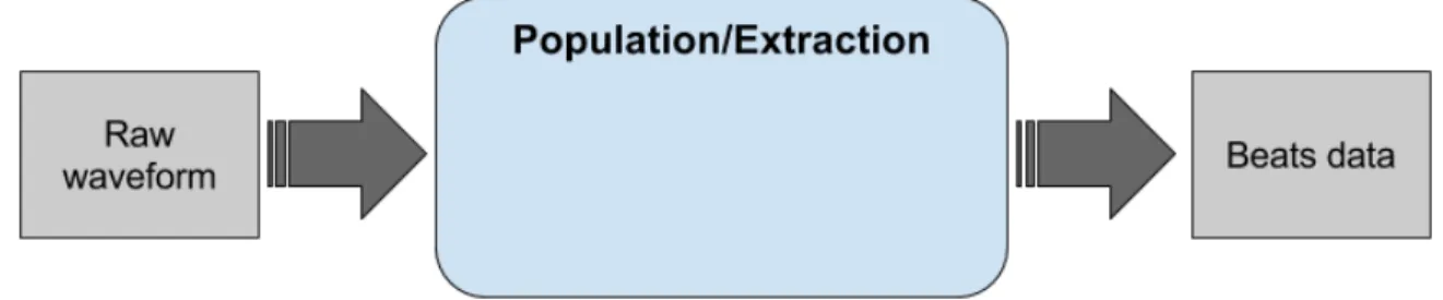
Figure 3-2: This figure shows a very simple diagram of the system overview of BeatDB v0. It only contains the population/extraction module, which takes in raw

waveform ABP data and outputs Beats data, with each beat object containing extracted features.

3.2.2 BeatDB v1

The first true iteration of BeatDB was primarily developed by Franck Dernoncourt and will be referred to as BeatDB v1 throughout this thesis. A more fleshed out ver-sion of the Beat Feature Database that Waldin proposed, BeatDB v1’s main

(38)

objec-tives were multi-level parameterization (primarily for flexibility of experimentation), lossless storage, and scalability.[7] It expanded upon the beat detection and feature extraction concepts presented in BeatDB v0 by adding a joint condition detection and feature aggregation module, introducing the rolling window condition detection algorithm used throughout future iterations of BeatDB (mentioned above in 3.1.2). For a diagram of the BeatDB v1 system overview, see figure3-3.

Given the first main objective of BeatDB listed above, this module was developed with flexibility to parameters in mind, allowing the user to specify the event to detect, which beat features to compute, how to aggregate features, and the machine learn-ing algorithms and evaluation metrics used to analyze the resultant dataset. Despite this, setting these parameters was not particularly user friendly, requiring users to have familiarity with the codebase to modify these arguments. As for its other main objectives, BeatDB v1 initially employed a master/worker architecture introduced by Waldin called DCAP (A Distributed Computation Architecture in Python)1 and later moved to a multi-worker architecture in which workers were synchronized by a com-mon result database in order to limit code overhead for connections between instances. To store lossless data, NFS servers were used so that workers could easily access data files in a shared way. Given the inexpensive nature of using OpenStack and NFS servers at CSAIL, BeatDB v1 was able to achieve scalability on large MIMIC-II ABP datasets.

Interestingly, BeatDB v1 had the most feature functionality of all iterations, ex-panding beyond condition detection and feature aggregation by directly computing a user-specified evaluation metric using a machine learning algorithm of the users choice. No future iteration has been concerned with providing this sort of analysis to users, focusing instead on the generation of a dataset that is immediately ready for machine learning analysis. Additionally, BeatDB v1 incorporated alternative complex methods of condition detection, using wavelets and a Gaussian process for parameter optimization on the same ABP problem to show the effectiveness of their

implementa-1

(39)

tions within the system. It is likely that these methods were not propagated forward to future iterations of BeatDB because of their much lower average AUROC scores compared to the rolling window condition detection algorithm and the complexity of implementation that each method required.

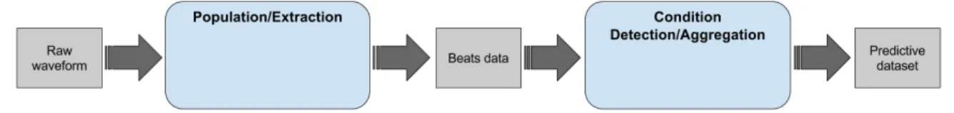
Figure 3-3: This figure shows a simple diagram of the two modules that comprise BeatDB v1. BeatDB v1 added onto BeatDB v0 by adding a condition detection/aggregation stage that outputs a predictive dataset of lag subwindows.

3.2.3 PhysioMiner

PhysioMiner is comprised of four major steps, outlined in detail throughout Gopal’s Master’s thesis and in documentation maintained by ALFA[3]. In each step, the PhysioMiner master instance creates or alters an existing DynamoDB table by adding messages to an SQS queue related to the step which are processed by worker instances who record and write results to the tables. Each step that occurs later in PhysioMiner is dependent on the tables generated by the steps before it. For a diagram and further explanation of the system architecture of PhysioMiner, refer to 3-5 at the end of this chapter.

What motivations were there for building PhysioMiner if a working version of BeatDB v1 existed? PhysioMiner is, more explicitly, the Amazon Web Services (AWS) system architecture used to run BeatDB, albeit a customized version of BeatDB that differs from v1 and is written in Java. As such, PhysioMiner is frequently referred to as an iteration of BeatDB rather than a framework that runs a BeatDB instance. Phys-ioMiner’s intent was not to overtake BeatDB but to provide a way to run the software on a modular and new (at the time) cloud service. As development progressed, Phys-ioMiner became an iteration of BeatDB in its own right, given that BeatDB was rewritten entirely within PhysioMiner. In this sense, PhysioMiner’s main motivation

(40)

was to expand BeatDB beyond the CSAIL servers and into a new cloud architecture with the hopes that the system could readily be used by a broader range of researchers than previously allowable with BeatDB v1.

Additionally, BeatDB v1 was not as user oriented as desired for a system meant to be used by numerous researchers on different projects. PhysioMiner allowed for users to customize each parameter as they called and initialized the script, giving the user more control over the system than BeatDB v1. Users were also allowed to create their own feature, aggregation, and filter functions in Python, which would be used by PhysioMiner for the stages it would run.

Rather than being broken up into two stages, as the conceptual BeatDB and BeatDB v1 did, PhysioMiner breaks BeatDB into four stages, consisting of population, feature extraction, condition detection, and feature aggregation. These steps can be seen as submodules of the two stages present in the other BeatDB iterations and are briefly discussed below.

Population

Population is the first step of PhysioMiner. It reads raw waveforms in the data folder of the root S3 bucket and populates a 𝑠𝑒𝑔𝑚𝑒𝑛𝑡𝑠 table. The 𝑠𝑒𝑔𝑚𝑒𝑛𝑡𝑠 table relates the raw waveform files to 𝑠𝑒𝑔𝑚𝑒𝑛𝑡_𝑖𝑑𝑠. Population also runs over each waveform and performs an onset detection algorithm to distinguish between the individual beats. Finally, PhysioMiner runs through the beats, extracting features from them that are specific to the signal type of the data while assigning a validity to them based on certain conditions.

A beat has one of three possible values in its 𝑣𝑎𝑙𝑖𝑑 field: 0 for invalid, 1 for valid, and 2 for gap (in the original PhysioMiner implementation, valid was a boolean and had no way of distinguishing between gap beats without directly checking the duration. See 3.3 for more details.). When considering ABP data, beats must pass validity checks related to having systolic pressure, duration, and other feature values

(41)

between acceptable ranges (this refers to an implementation of the signal abnormality index mentioned in 2.2.2). If the beat has a duration of greater than 6 seconds, which is impossible for a human heartbeat and implies some sort of loss of signal or disconnection from the sensors, then the beat is assigned a validity of 2.[31] Once all beats have been analyzed for validity, they are written to a 𝑏𝑒𝑎𝑡𝑠 table in DynamoDB.

Feature Extraction

The next step is feature extraction, which iterates over a specific 𝑏𝑒𝑎𝑡𝑠 table and adds additional features, specified by the user, to each beat based on analysis of each waveform. Features to be added must be specified in the command that runs feature extraction. Each feature must have a corresponding Python script containing its logic placed in a subfolder for the data type (ABP, ECG, etc) inside of the 𝑓 𝑒𝑎𝑡𝑢𝑟𝑒𝑠/ folder in the S3 bucket. When feature extraction is run, it will add values for the new features not yet present in each individual row in the 𝑏𝑒𝑎𝑡𝑠 table and overwrite values for features with the same name that have been recalculated (if the script has not changed, it will overwrite with the same information assuming the raw input data is the same).

This step is run in conjunction with population by default but can be rerun afterward to add more features to the individual beats in the specified 𝑏𝑒𝑎𝑡𝑠 table. Population and feature extraction can be seen as two submodules of the Beat Object Generation module in the conceptual view of BeatDB discussed in 3.1.

Condition Detection

The third step in PhysioMiner is condition detection. This step is described as it exists in the latest update to PhysioMiner, and differs from its original implementation (see

3.3). When a beat is checked for validity, it may be flagged as a gap beat, described in the population step above. If a beat is a gap beat, any beats after and including this gap beat may not be part of a contiguous segment as the duration of the gap beat indicates a loss of signal. In order to only consider valid groups of the patient’s raw

(42)

waveform, PhysioMiner must preprocess the waveform and find where gap beats occur and where these gap sections end. A valid beat group is a section of the patient’s raw waveform starting with a valid beat and containing no gap beats. This guarantees that valid beat groups are contiguous sections of the waveform and are not noise.

After generating the valid beat groups (VBGs), a sliding window algorithm is run over each of them. The sliding window is initially formed at the start of the VBG, with PhysioMiner calculating the sliding window’s end beat by considering the duration of lag, lead, and the condition window. If the end beat is beyond the bounds of the VBG, the algorithm continues to the next VBG. If our sliding window fits in the VBG, the condition is determined from the condition window using a condition script. If the condition window matches the condition, the window is saved and the sliding window is moved forward by an entire sliding window length so that it starts at the end beat of the current sliding window. Otherwise, the sliding window is only moved ahead by 𝑙𝑎𝑔 seconds.

For example, let’s assume a sample waveform has 800 seconds of data and no gaps and the lag and lead durations are both 10 s while condition window length is 60 s. Assume that the first group window (the first step of our rolling window algorithm) starts at the very first beat, and each beat is 1 second long. Detecting the condition in the condition window would make the next rolling window start at the 81st second (jumping over the condition window entirely), while not detecting the condition would make the next rolling window start at the 11th second (moving ahead by lag seconds). If gaps had existed in this waveform, the algorithm would simply check if a gap beat existed in the group window’s range every time it had a new start index, and if there was a gap beat in its range, the algorithm would start the group window at the first valid beat after this gap beat. A simplified visual representation of this can be seen in figure 3-4.

Once the end of the last VBG is reached, a user-defined filter script may run on the discovered windows, allowing the user to only see a specific number of windows

(43)

Figure 3-4: This image shows how VBGs are found and used in condition detection. 1 shows a waveform being split into valid beat groups and invalid/gap sections (a

section that starts with a gap beat). 2 shows the first VBG being processed by condition detection, which starts by placing the sliding window at the start of the VBG and then running the sliding window algorithm on the VBG until the window

reaches the end of the VBG. Afterward, the sliding window algorithm starts at the start of the next VBG and is run until it reaches the end of the VBG, as shown in 3.

By only detecting conditions over VBG’s, we ensure that the generated dataset contains data containing the least noise and possibly save on computation time by

not needlessly generating data over invalid regions.

matching some sort of user-defined criteria. Finally, the resultant windows are written to the 𝑤𝑖𝑛𝑑𝑜𝑤𝑠 table (with no filter script, all windows are written). Each sliding window is represented by a row in the 𝑤𝑖𝑛𝑑𝑜𝑤𝑠 table, with each row containing information such as the condition classification, beat id’s of the start and end beats, lead, lag, and condition window length. (In the original PhysioMiner implementation, each sliding window in the 𝑤𝑖𝑛𝑑𝑜𝑤𝑠 table did not contain lag or lead since each entry was only representative of the condition window. See 3.3.2 for more details.)

(44)

Feature Aggregation

The last step of BeatDB is feature aggregation. Feature aggregation reads from the 𝑤𝑖𝑛𝑑𝑜𝑤𝑠 table generated in the previous step with the aim of aggregating features over each predictor (lag) window. Users specify how many subwindows the lag win-dow will be divided into and which user-defined aggregator functions to run over specified features from the extraction step. New, aggregate features for each subwin-dow from the lag winsubwin-dow are generated, with each group winsubwin-dow existing as a row in the 𝑤𝑖𝑛𝑑𝑜𝑤𝑠 table. The number of new features added to each row is found by multiplying the number of aggregator functions by the number of features, and the number of new rows is found by multiplying the number of rows in the windows col-umn by the number of subwindows. For example, if the user picked two subwindows and supplied four aggregators and two features, the new dataset would have twice as many rows as the windows table and each row would have 8 more features (one aggregate feature is created for each feature and aggregator pair).

After generating the lag window aggregate features, a row with the old and new fea-tures for each subwindow is added to the 𝑤𝑖𝑛𝑑𝑜𝑤𝑠_𝑙𝑒𝑎𝑑_𝑥_𝑙𝑎𝑔_𝑦_𝑠𝑢𝑏𝑤𝑖𝑛𝑑𝑜𝑤𝑠_𝑧 table, where 𝑥 is lead in seconds, 𝑦 is lag in seconds, and 𝑧 is number of subwindows. Since each window and subwindow still has the same classification as generated in condition detection for it’s parent group window, this table is useful for learning, as one can use the aggregate features to try to predict the label. Using additional processing scripts, the user can generate a .csv file from the table and port it into any machine learning framework for analysis, keeping in mind the columns that need to be removed or ignored for processing, such as those containing id values and other string-based information.

3.3 Modifications to PhysioMiner

After completing the implementation of PhysioMiner, the system was tested using ECG data. However, PhysioMiner did not adequately test the accuracy of generated

(45)

datasets when using the ABP data from the BeatDB v1 experiments. The first major task of this thesis work required searching for the NFS server used with BeatDB v1 for code or experiment results from Dernoncourt’s work. In this process, inconsistencies between BeatDB v1 and PhysioMiner were found and investigated, leading to further implementation on the PhysioMiner platform. This section details the comparison between PhysioMiner and BeatDB v1, leading to the discovery of the cause of the inconsistencies, and a high-level overview of the process of modifying PhysioMiner, giving an analysis of its results.

3.3.1 Comparison with BeatDB v1

Despite the searches through the lab’s NFS server, code for onset detection, the wavelet feature implementation, and other internal processes were discovered, but a complete working copy of BeatDB v1 was not found. However, a significant amount of resultant aggregated datasets created by BeatDB v1 were found, allowing for compar-ison between the output of PhysioMiner and BeatDB v1. Given the major differences between the design and frameworks used for computation, the BeatDB v1 output data looks different than the PhysioMiner output data, but there are valid explana-tions for most of the differences.

Given the cost of repopulation, both monetarily and temporally, we are comparing two resultant datasets that already existed (in the case of the PhysioMiner implemen-tation, the large scale 𝑏𝑒𝑎𝑡𝑠 and 𝑤𝑖𝑛𝑑𝑜𝑤𝑠 tables already existed, with the aggregation table being created to match the parameters of the BeatDB v1 result file). On the left is the result of learning on the data from the NFS server that Dernoncourt used to develop BeatDB initially. The right side contains the results of learning on the output of the original implementation of PhysioMiner. These tests are meant to compare the effectiveness of learning algorithms on resultant datasets from the different iterations of BeatDB.

(46)

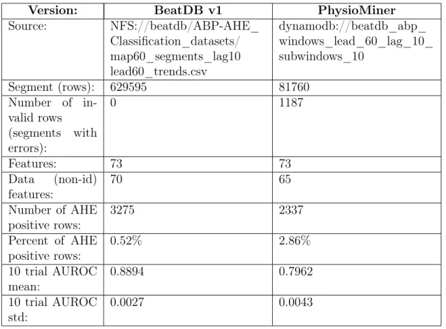
Version: BeatDB v1 PhysioMiner Source: NFS://beatdb/ABP-AHE_ Classification_datasets/ map60_segments_lag10 lead60_trends.csv dynamodb://beatdb_abp_ windows_lead_60_lag_10_ subwindows_10 Segment (rows): 629595 81760 Number of in-valid rows (segments with errors): 0 1187 Features: 73 73 Data (non-id) features: 70 65 Number of AHE positive rows: 3275 2337 Percent of AHE positive rows: 0.52% 2.86% 10 trial AUROC mean: 0.8894 0.7962 10 trial AUROC std: 0.0027 0.0043

Table 3.1: Comparison of resultant datasets from BeatDB v1 and PhysioMiner.

PhysioMiner achieves an AUROC score 9% lower than BeatDB v1, which indicates a problem somewhere in the workflow. BeatDB v1 appears to generate significantly more segments than PhysioMiner, which may indicate that it was designed less ef-ficiently in some way. This difference in design makes sense, seeing as PhysioMiner runs on AWS, which requires money to use, while BeatDB v1 used OpenStack and NFS servers already available at CSAIL for its distributed tasks. The large number of segments generated by BeatDB v1 may indicate that Dernoncourt did not skip over the condition window for the next rolling window entirely if the condition was detected in the condition detection algorithm. This may have an effect on AUROC and the number of AHE positive rows. (In the initial programming for the imple-mentation of valid beat groups in PhysioMiner, discussed in 3.3.2, a similar mistake resulted in about 10 times more rows in the final dataset, making the process very costly and inefficient but providing giving evidence that this may have resulted in the large output table from BeatDB v1.)

(47)

Additionally, five data features are missing in PhysioMiner. The missing features are the five aggregation values for duration, since duration is calculated internally by BeatDB v1 and the aggregation step in PhysioMiner requires that the features are user-defined, meaning that PhysioMiner would not aggregate duration. PhysioMiner stores 5 extra variables (𝑏𝑒𝑎𝑡_𝑠𝑡𝑎𝑟𝑡_𝑖𝑑, 𝑏𝑒𝑎𝑡_𝑒𝑛𝑑_𝑖𝑑, 𝑐𝑜𝑛𝑑𝑖𝑡𝑖𝑜𝑛_𝑤𝑖𝑛𝑑𝑜𝑤_𝑙𝑒𝑛𝑔𝑡ℎ, 𝑠𝑢𝑏𝑤𝑖𝑛𝑑𝑜𝑤_𝑖𝑛𝑑𝑒𝑥, and 𝑤𝑖𝑛𝑑𝑜𝑤_𝑙𝑒𝑛𝑔𝑡ℎ), which results in both datasets having 73 features with only 68 of the features (the 65 data features and 3 ID values) in common between the datasets.

These results prompted a direct comparison of the code and processes used in BeatDB v1 and PhysioMiner. Waldin’s thesis gave significant background to the window find-ing algorithm, and analysis of it showed that PhysioMiner was lackfind-ing gap beat detection, meaning that some windows contained invalid sections of the waveform and should not have been included in resultant datasets. This could be one reason for the large difference in AUROC scores and is further explored in the next section.

3.3.2 Valid Beat Groups (VBGs)

In the port from BeatDB v1 to PhysioMiner, the condition detection step was changed, modifying the way windows are found over a waveform. The change is subtle, but seemingly has a large effect on the AUROC scores of the resultant dataset.

In BeatDB v1, condition detection runs the sliding window algorithm over contigu-ous segments of the waveform only. Contigucontigu-ous segments of the waveform were easily identifiable because the beats database had a different schema, which created the 𝑣𝑎𝑙𝑖𝑑 field as an integer instead of a boolean. If 𝑣𝑎𝑙𝑖𝑑 had a value of 2, it meant that the beat was a gap beat, indicating that it had a duration of 6 seconds or more. Gap beats are likely the result of an error, either in the device or with the patient (removal of the detectors, etc. See 2.2.1 for more information) and were discarded from consideration. This allowed for the condition detection step to be more efficient and made the data more meaningful as it was guaranteed to come from signal rather

(48)

than noise. Additionally, the sliding window in condition detection had a size of 𝑙𝑒𝑎𝑑 + 𝑙𝑎𝑔 + 𝑐𝑜𝑛𝑑𝑖𝑡𝑖𝑜𝑛_𝑤𝑖𝑛𝑑𝑜𝑤_𝑙𝑒𝑛𝑔𝑡ℎ seconds, essentially bundling the condition window with the predictor (lag) window in the database. (This is a group window based on the definition and diagram in 3.1.2) If this group window concept is carried forward to future iterations of BeatDB, it could be used to do condition detection and feature aggregation simultaneously, cutting down on overall file processing time.

In the Java implementation, the 𝑣𝑎𝑙𝑖𝑑 field in the 𝑏𝑒𝑎𝑡𝑠 tables is a boolean, losing the capability to distinguish between gap beats and normal beats. Instead, the condition detection step starts at or near the beginning of the file, depending on the value of the 𝑔𝑎𝑝 argument, which can be used to start from a constant offset from the start of the waveform. The algorithm does not manually check beat duration for gap beats, so the windows formed come from the entire waveform, not just the contiguous beat sections. This could be the reason for the difference in AUROC score and database sizes between the resultant datasets from the Python and Java implementations of BeatDB, as the Java implementation used for testing includes invalid windows.

To test this idea, an instance of PhysioMiner’s implementation from August 2016 and an updated version with valid beat groups implemented were compared. The result of linear regression on the aggregated windows tables from each version is shown in table 3.2.

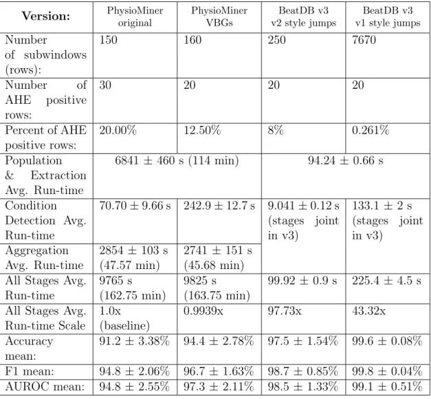
One result from a learning trial for each version of BeatDB is provided to show sam-ple output of the learning process used, but keep in mind that the valid beat group version did not always outperform the original version and the difference was not always as great as 2% in AUROC. However, the average over ten trials shows a clear increase by 1% in the VBG version, which may indicate that VBGs are necessary for BeatDB’s overall accuracy. The standard deviation for the VBG version is smaller by a factor of 20, meaning that it is more consistent with its AUROC score than the version that does not look for gap beats.

(49)

Version: PhysioMiner (original) PhysioMiner (VBGs) Sample files

pro-cessed:

3000000.edf, 3000002.edf, 3000105.edf, 3900017.edf

Rows: 150 160 Number of AHE positive rows: 30 20 Percent of AHE positive rows: 20.00% 12.50% 10 trial AUROC mean: 0.9699 0.9797 10 trial AUROC std: 0.0197 0.0096

Table 3.2: Comparison of original PhysioMiner implementation and PhysioMiner with valid beat groups (VBGs). This data was generated using a lead of 60 s, a lag of 10 s, and 10 subwindows, meaning that the predictor (lag) window was split into

10 sections for feature aggregation.

Why were VBGs left out of PhysioMiner when it is based off from BeatDB v1? Perhaps the 𝑔𝑎𝑝 argument was confused with the gap beat concept during the im-plementation of the Java port and the detail of the 𝑣𝑎𝑙𝑖𝑑 field for each beat ob-ject having three possible values was lost, preventing PhysioMiner from iterating over valid sections of the waveform while skipping invalid ones. Because of this, lead and lag were not required as arguments for condition detection, which resulted in the sliding window containing only the condition window with a duration of 𝑐𝑜𝑛𝑑𝑖𝑡𝑖𝑜𝑛_𝑤𝑖𝑛𝑑𝑜𝑤_𝑙𝑒𝑛𝑔𝑡ℎ seconds.

Not requiring lead and lag as arguments for condition detection forced the software to aggregate features by looking backwards in the raw waveform to find prediction windows. Instead, the software should have given the indices of the prediction win-dow by coupling it with the condition winwin-dow in the winwin-dows database. This could be the cause of significant inefficiencies. In future iterations of BeatDB, this must be considered, as the new requirement of lead and lag in condition detection could allow it to be performed simultaneously with feature aggregation while only considering contiguous sections of the waveform.

(50)

Figure 3-5: This figure, created by Alejandro Baldominos[4], shows the general PhysioMiner system architecture for both master and worker instances. Master instances start by creating worker EC2 instances and then gather items from DynamoDB in order to determine what needs to be processed. Once this has completed, the master instance uploads messages describing each task to the SQS

queue. Worker instances spawn by receiving the PhysioMiner JAR file from S3 along with a message from the SQS queue, which prompts the workers to pull the

specified items from DynamoDB and process them. Once this has completed, the workers write to the resultant DynamoDB table and continue to fetch and process

(51)

Chapter 4 BeatDB v3

BeatDB v3 is a new iteration of the BeatDB system, fully written in Python and designed with efficiency (correctness and performance), more complex feature ex-traction, and high code coverage as focuses of the project. It consists of a popula-tion/extraction stage and a condition detection/aggregation stage. Additionally, a standalone preprocessing stage, developed primary by Alejandro Baldominos, and a standalone file size reader were developed for use with BeatDB v3. This chapter will focus on motivations for creating a third iteration of BeatDB and then present a sys-tem overview along with a discussion regarding new features and optimizations made. Technical specifics for BeatDB v3, including how to run the software, implementation details, and other technical information, can be found in appendix A.

4.1 Motivations

Primary motivations for developing a new iteration of BeatDB v3 were initially related to extending the functionality of PhysioMiner. In order to add more flexibility to the system, developers wanted to add the capability to extract channel and multi-sample/temporal features (where a chunk is a specific slice of the raw waveform (a beat would be considered a subset of a chunk)) and make it simpler for users to define their own signal types. However, given the large codebase and the amount of architectural complexity written within PhysioMiner, adding features to the system

BeatDB v3 : a framework for the creation of predictive datasets from physiological signals

BeatDB v3: A Framework for the Creation of

Predictive Datasets from Physiological Signals

by

Steven Anthony Rivera

S.B., Massachusetts Institute of Technology (2016)

Submitted to the Department of Electrical Engineering

and Computer Science

in partial fulfillment of the requirements for the degree of

Master of Engineering in Computer Science and Engineering

at the

MASSACHUSETTS INSTITUTE OF TECHNOLOGY

June 2017

c

○ Massachusetts Institute of Technology 2017. All rights reserved.

Author . . . .

Department of Electrical Engineering

and Computer Science

May 26, 2017

Certified by . . . .

Una-May O’Reilly

Principal Research Scientist

Thesis Supervisor

Certified by . . . .

Erik Hemberg

Research Scientist

Thesis Supervisor

Accepted by . . . .

Christopher J. Terman

Chairman, Masters of Engineering Thesis Committee

BeatDB v3: A Framework for the Creation of Predictive

Datasets from Physiological Signals

by

Steven Anthony Rivera

Abstract

Acknowledgments

Contents

List of Figures

List of Tables

Chapter 1

Introduction

1.1

Development Background

1.2

Objectives

1.3

Organization

Chapter 2

Background

2.1

Related Work

2.1.1

Feature Engineering

2.1.2

Prediction of Medical Events

2.1.3

Computing Frameworks

2.2

Medical Data

2.2.1

Issues with Waveform Data

2.2.2

Using the Data

Chapter 3

BeatDB

3.1

BeatDB Design

3.1.1

Beat Object Generation

3.1.2

Dataset Preparation

3.2

Previous Implementations

3.2.1

BeatDB v0

3.2.2

BeatDB v1

3.2.3

PhysioMiner

3.3