HAL Id: halshs-02934878
https://halshs.archives-ouvertes.fr/halshs-02934878
Submitted on 9 Sep 2020
HAL is a multi-disciplinary open access
archive for the deposit and dissemination of sci-entific research documents, whether they are pub-lished or not. The documents may come from teaching and research institutions in France or abroad, or from public or private research centers.
L’archive ouverte pluridisciplinaire HAL, est destinée au dépôt et à la diffusion de documents scientifiques de niveau recherche, publiés ou non, émanant des établissements d’enseignement et de recherche français ou étrangers, des laboratoires publics ou privés.
Scrutinizing the Direct Rebound Effect for French
Households using Quantile Regression and data from an
Original Survey
Fateh Belaïd, Adel Ben Youssef, Nathalie Lazaric
To cite this version:
Fateh Belaïd, Adel Ben Youssef, Nathalie Lazaric. Scrutinizing the Direct Rebound Effect for French Households using Quantile Regression and data from an Original Survey. Ecological Economics, Elsevier, 2020, 176, pp.106755. �10.1016/j.ecolecon.2020.106755�. �halshs-02934878�
Scrutinizing the Direct Rebound Effect for French Households using Quantile Regression and data from an Original Survey
Dr. Fateh BELAID*
Faculty of Management, Economics & Sciences
Lille Catholic University, UMR 9221-LEM-Lille Économie Management F-59000 Lille, France. Email: fateh.belaid@univ-catholille.fr / fateh.belaid@univ-littoral.fr
Dr. Adel BEN YOUSSEF
Université Côte d'Azur, CNRS, GREDEG (UMR, 7321), Nice, France E.mail : adel.ben-youssef@gredeg.cnrs.fr
Dr. Nathalie LAZARIC
Université Côte d'Azur, CNRS, GREDEG (UMR, 7321), Nice, France E.mail : nathalie.lazaric@gredeg.cnrs.fr
*Dr. Fateh BELAÏD, Corresponding author
Faculty of Management, Economics & Sciences
Lille Catholic University, UMR 9221-LEM-Lille Économie Management F-59000 Lille, France.
Scrutinizing the Direct Rebound Effect for French Households using Quantile Regression and data from an Original Survey
Abstract
This article develops a quantile regression model to measure the magnitude of the direct rebound effect for residential electricity demand based on micro-level data from an original survey of a representative sample of 2,356 French households. We explore the rebound effect for different groups of residents. Traditionally, debate has focused on decreased prices for energy services due to efficiency improvements and their effects on energy demand. The methodological innovation provided by this paper is that it implements two theoretical estimation strategies: (i) energy efficiency elasticity of the demand for energy services, and (ii) price elasticity of the demand for energy services. Our findings reject the hypothesis of a backfire effect in the context of residential electricity use. Specifically, based on energy efficiency elasticity, we provide evidence of a rebound effect of between 72% and 86% but with substantial heterogeneity among consumption quantiles. Our results show that the direct rebound effect has critical relevance for energy efficiency policy in the face of energy invisibility in France.
Keywords. Energy efficiency; Rebound effect; Quantile regression; Residential energy consumption; Household behavior.
1. Introduction
For several world countries, improving the energy efficiency1 of their housing stock has for long been considered an effective strategy to reduce demand for residential energy and achieve sustainability goals (Sorrell and Dimitropoulos, 2008; Estiri, 2014; Belaïd and Garcia, 2016; Volland, 2017, Belaïd, 2016, 2017). However, this policy of reducing demand for energy by promoting resource and energy efficiency has mostly failed to live up to expectations. One of the most frequent explanations for this failure is the “rebound effect” according to which increased housing energy efficiency does not necessarily translate into a corresponding decrease in the demand for energy in absolute terms (Sorrell and Dimitropoulos, 2008; Turner, 2013; Borenstein, 2015, Belaïd et al., 2018). In this context, the rebound effect can be defined also as the “unintended consequences of actions by households to reduce their energy consumption and/or greenhouse gas (GHG) emissions” (Sorrell, 2010, p. 8). The rebound effect can be considered a mainly attitudinal and behavioral response to an improvement in energy efficiency2. Therefore, the potential level of savings depends on these efficiency-induced attitudinal and behavioral effects.
There is no consensus in the literature about the magnitude of the rebound effect, and its theoretical foundations continue to be debated. Previous empirical findings suggest that households which increase their energy efficiency also increase their consumption of energy
1 Energy efficiency is the inverse of energy intensity which is defined as the ratio of energy input to
monetary output.
2 The rebound effect refers to the proportionate rise in demand for energy services following an
endogenous diminution in the marginal cost of supplying the service due to energy efficiency improvements of a given proportion. The rebound effect includes both system and household behavioral responses to reductions in the cost of energy services as a result of energy efficiency improvements.
(Greening et al., 2000; Binswanger, 2001; Hertwich, 2005; Peters et al., 2012; Sorrell, 2007 and others). This has been explained as due to energy invisibility (Hargreaves et al., 2010), behavioral “lock in” (Maréchal, 2010; Maréchal and Lazaric, 2010), habitual practices (Maréchal and Holzemer, 2015, Lévy and Belaïd, 2018, Belaïd and Joumni, 2020), consumer inattention to energy efficient technologies (Sallee, 2014; Davis and Metcalf, 2016; Burlinson et al., 2018 a, b), social status and identity (Filippín et al., 2018).
The extensive empirical literature includes differences in how the rebound effect is defined, lack of or poor quality of data and different empirical methodologies used for the estimations. There is remarkable agreement among energy economists that the problems related to quantifying the rebound effect are due mainly to inadequate data, uncertain causal relationships, and other difficulties (Sorrell, 2007). As a result, the existing literature is fragmented and limited mostly to direct rebound effects because estimation of indirect effects requires general equilibrium adjustments which are not easy to capture empirically (Sorrell and Dimitropoulos, 2008; Zhang et al., 2017; Lin et al., 2013). In our case, our data do not allow us accurately to assess the indirect rebound effect related to reuse of energy cost savings for other services, goods and production factors (Thomas and Azevedo, 2013; Sorrell and Dimitropoulos, 2008), e.g. cost savings spent on cooking or overseas holidays which both use additional energy. Further, while the direct rebound effects are derived from econometric analysis of survey data on household expenditure, the indirect rebound effects are derived from a combination of life cycle analysis (LCA) and environmentally-extended input-output models. Existing empirical studies tend to measure direct and indirect rebound effects jointly using mainly times series and panel data and a system of demand models for energy and other
goods such as the almost ideal demand system (AIDS) model proposed by Deaton and Muellbauer (1980). To estimate the indirect rebound effect using cross-sectional data requires three sets of data (Nässén and Holmberg, 2009) on (i) share of marginal household expenditure, (2) energy intensity of the goods and services consumed, and (3) energy service price elasticity. Unfortunately, our survey data do not provide all of this information.
The objective of this paper is to estimate the direct rebound effect accurately. It employs quantile regression to measure the magnitude of the direct rebound effect on French residential electricity consumption and micro-level data from an original individual household survey (PHEBUS Survey 2014)3. The proposed quantile model helps to differentiate the effects of several variables on the entire consumption distribution. The main sample includes 2,356 households in housing units selected to ensure 4 representativeness of French principal residential dwelling stock. PHEBUS was designed by the French government to improve knowledge regarding the energy efficiency of existing building stock. One of the authors of this paper was involved in the design of the PHEBUS questionnaire and assessment of the survey results. PHEBUS is the only survey in France which includes both actual and theoretical energy consumption measured using the energy performance diagnosis (EPD). The EPD provides information on the energy efficiency of particular buildings, and a rating system on a scale of A to G where A is high energy efficiency and G is low energy efficiency. “A” EPD category is required for all new build, rental or for sale French residential and
3 PHEBUS (Enquête Performance de l’Habitat, Équipements, Besoins et Usages de l’énergie) - Housing
commercial buildings. Table 1 shows the distribution of the French housing stock by energy label, based on the PHEBUS survey (Annex 1).
This paper makes several contributions. First, we propose a new dimension to explore the spectrum of household electricity consumption and the link between policy and household behavior. Second, we discuss the electricity consumption rebound effect in France which in 2015 was one of the EU countries with the highest levels of total electricity consumption (436.19 billion kWh) (Eurostat, 2017). Empirical research on the rebound effect and the effects of dwelling- and household-related factors on domestic electricity consumption in France, is limited due to lack of information and availability of disaggregated data on household electricity consumption. Third, we examine the effects of household behaviors, dwelling and climate on residential electricity consumption. Fourth, by separating the effects on domestic energy demand of energy efficiency and energy pricing, our original empirical findings contribute to debate over whether households respond differently to energy efficiency improvements and changes to energy prices. Chan and Gillingham (2015) demonstrate that compared to service prices and efficiency elasticity of the demand for services, demand for services and price elasticity capture essentially distinct implicit price changes. Our empirical results show high average rebound effect values for electricity consumption in France ranging between 38% and 86% (38%-71% for price elasticity, and 72%-86% for efficiency elasticity), and confirm previous findings for the rebound effect in the OECD countries. Also, our results suggest substantial heterogeneity among consumption quantiles. These are in line with previous work showing the sensitivity of the rebound effect to income group (Small and Dender, 2007; Gillingham, 2011; West, 2004; Kulmer and Seebauer, 2019), and suggesting
inequalities in energy consumption (Chester, 2014; Sovacool et al., 2017; Reyes et al., 2019) with potentially diverse rebound effects.
The paper is organized as follows: section 2 reviews the literature and discusses microeconomic rebound effect theory. Section 3 describes the data and the analytical methods, and section 4 presents the findings. Section 5 concludes the paper with a discussion of the findings.
2. Theoretical background and empirical evidence of the rebound effect
This section summarizes the theoretical background to the rebound effect and surveys the empirical evidence. Research on the rebound effect is essential to provide the knowledge needed to improve evidence-based energy policy and energy efficiency strategies related to the residential sector.
2.1. Theoretical background
The rebound effect has been high on the agendas of policy makers and academics since the early 1980s but originated in Jevons’s (1865) seminal piece. Jevons pointed out that although the coal-fired steam engine had improved production efficiency greatly, its widespread use had led to increased consumption of coal. However, research into the rebound effect did not begin until the late 1970s. Brookes’s (1978) and Khazzoom’s (1980) pioneering works suggested that if the price of energy remained unchanged, energy efficiency improvements caused by technological advancements would increase rather than reduce energy consumption. Since then, the number of empirical and theoretical papers on the rebound effect in different sectors (e.g. personal automotive transport, household heating, space cooling, other household energy services, etc.) based on different types of data (e.g. aggregate or
household level, cross section or time series, etc.) has increased as there is interest in definition and measurement of the phenomenon.
Microeconomic work on the rebound effect highlights that income and the substitution effect help to explain how the rebound effect influences users’ attitudes and behaviors. The link between a reduction in energy prices and changes to incomes is depicted in the Slutsky decomposition (Thomas and Azevedo, 2013) (see fig. 1 for the two Slutsky relations). To demonstrate the direct rebound effect in the case of normal goods, we suppose that the original budget constraint A which is a function of the energy efficiency improvement, moves outward to B which is the result of a decrease in the price of energy services due to an increase in energy efficiency. At a level of utility𝑈0, this implies that maximizing the consumption bundle changes from 𝐸0(𝑄0, 𝑆0) to 𝐸1(𝑄1, 𝑆1) which represents a higher level of utility (𝑈1) for the individual. Variation in energy services demand can be decomposed into: (i) a substitution effect, and (ii) an income effect. The substitution effect refers to the variation in demand for energy services, holding utility constant i.e. keeping purchasing power fixed. The income effect refers to the variation in demand for energy services to achieve a higher level of utility. The resulting net change in energy services demand (combined substitution and income effects) is defined as the direct rebound effect.
Fig.1. The rebound effect Slutsky decomposition i.e. substitution and income effect induced by an energy price drop
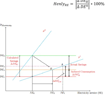
Based on similar reasoning, we can explore the change in “other services” with respect to a variation in the energy price to obtain the indirect rebound effect which results from a similar decomposition of cross-price elasticities of the demand for other energy services. The implications of the direct and indirect rebound effects on energy consumption are depicted in fig. 2 based on Khazzoom’s (1980) and Henly et al.’s (1988) theoretical formulations of the rebound effect.
First, assuming original demand was at 𝐷𝐸0, Khazzoom’s formulation suggests that energy efficiency improvements will increase electricity services from 𝑆𝐸0 to 𝑆𝐸1 which induces an increase in electricity demand from 𝐷𝐸1 to 𝐷𝐸2. That is, the householder will consume electricity at point 𝑨(𝑆𝐸1, 𝐷𝐸2).
Assuming that ∆ 𝐷𝐸0(𝐷𝐸0− 𝐷𝐸1) is the electricity demand saving for an improvement in energy efficiency and ∆ 𝐷𝐸𝐾ℎ1 (𝐷𝐸2− 𝐷𝐸1) is the increase in demand for electricity induced
by a decrease in the price of electricity, Khazzoom's direct rebound effect can be formulated as follows:
𝐾ℎ𝑎𝑧𝑧𝑜𝑜𝑚𝑅𝐸 = |
∆ 𝐷𝐸𝐾ℎ1
∆ 𝐷𝐸0 | ∗ 100%
Second, in the case of the Henly formulation, an improvement in energy efficiency will increase demand for electricity services. However, because of the increase in the cost of electricity services above the capital cost, consumption will decrease from 𝑆𝐸0 to 𝑆𝐸2. Therefore, the user will consume electricity at 𝑩(𝑆𝐸2, 𝐷𝐸3), and the change in electricity demand will be equal to ∆ 𝐷𝐸𝐻1(𝐷𝐸
3− 𝐷𝐸1). Henly’s direct rebound electricity effect is given by:
𝐻𝑒𝑛𝑙𝑦𝑅𝐸= | ∆ 𝐷𝐸𝐻1
∆ 𝐷𝐸0| ∗ 100%
Fig. 2. Interactions among price decreases, electricity demand, efficiency improvements, and the rebound effect
From an analytical perspective, several papers try to identify rebound effect types (Khazzoom, 1980; Brookes, 1978; Greening et al., 2000; Sorell and Dimitriopoulos, 2008; Antweiler and Gulati, 2016; De Borger et al., 2016). The economic literature distinguishes between direct effects, indirect effects and transformational effects.
The direct effect as defined by Khazzoom, refers to increased demand for an energy service
following an improvement in the efficiency of that energy service. More precisely, it represents the change in energy consumption resulting from the combined income and substitution effects on demand for an energy-efficient product (Sorell and Dimitriopoulos, 2008; Gillingham et al., 2016).
The indirect effect subsumes the effect of an energy efficiency increase on the demand for all
other goods and services, and the subsequent change in energy consumption (Gillingham et
al., 2016). The energy literature is not consistent in its use of this term. Some analyses incorporate any transformation in energy consumption driven by transformations in other services and goods including income effects, substitution effects and any incorporated energy used to achieve an improvement in energy efficiency (Azevedo, 2014; Gillingham et al., 2016). Other scholars employ the term “indirect rebound effect” more broadly to include, income effects, substitution effects, embodied energy and macroeconomic rebound effects (Sorrell and Dimitropoulos, 2008). However, the most frequent definition in the energy efficiency literature emphasizes the indirect rebound effect as incorporating only revenue effects on the demand of all other services and goods.
Finally, the economy-wide effect is defined broadly as an increase in energy demand induced by an energy efficiency upgrade via innovation and market adjustment channels. However,
according to Gillingham et al. (2016), the economy-wide effect is complex, and our understanding of it remains limited. In addition, the empirical evidence supporting this rebound effect is minimal because the interconnected complex global economic dynamic system virtually undermines arguments about effect and cause. Indeed, market adjustments causing changes in demand for energy, and energy efficiency improvements can affect overall energy demand through several adjustment channels.
Although our understanding of the rebound effect has improved significantly, debate over its magnitude persists and has crucial implications for energy efficiency policy. To respond to calls in the recent literature and to inform this debate, the present study provides an estimate of the magnitude of the rebound effect using definitions of both price and energy efficiency elasticities, and explores how these vary among diverse household groups.
2.2. Empirical evidence of the rebound effect
There is a large literature on the direct rebound effect5 related to energy consumption (Khazzoom, 1986; Haas and Biermayr, 2000; Galvin, 2015), and a significant stream of work on electricity consumption (mostly for the case of China).
5 While in the present paper we examine only the direct rebound effect, it is worth noting that there is a
strand of literature which considers the difference between the direct and indirect rebound effects. E.g. Lin et al. (2013) disaggregate the rebound effect into the direct and indirect effects based on all household commodities. They find that the rebound effect related to Chinese urban households is approximately 22%. The originality of their work given data availability, is the decomposition into direct and indirect effects (respectively 4.5% and 17.5%). Zhang et al. (2017) estimate the total provincial level CO2 rebound effect for China's private cars during 2001–2012 and find that the direct CO2 rebound effect plays a dominant role in the total CO2 rebound effect in most provinces. It should be noted that they found important differences between direct and indirect rebound effects. These findings suggest the need if the data allow, for careful consideration of these two measures to achieve a better understanding of the rebound effect.
For example, Wang et al. (2014) demonstrate the existence of a rebound effect in the context of residential electricity consumption in China during the period 1996 to 2010. The long-term rebound effect is 74% and the short-term rebound effect is 72%. Also, for the case of China, Zhang and Peng (2016) find a similar direct rebound effect for the period 2000-2013 averaging around 71% but varying with income regime, rainfall and colder days. Focusing on Beijing and using an input-output model, Wang et al. (2016) find that residential electricity use in Beijing exhibits a partial rebound effect, with respective long-term direct and indirect rebound effects of 46% and 0.56%, and short-term direct rebound effects of 24% and 37%.
Han et al. (2019) use Chinese panel data for urban residential electricity consumption and provide an improvement to calculation of the rebound effect based on price decomposition and spatial econometrics. They show that the direct rebound effect and its spillover effects (energy consumption dependence among regions) are respectively 37% and 13%, suggesting that the main factor affecting energy efficiency implementation is the direct rebound effect driven by the local region, and that the spillover effect is low. On the other hand, elimination of the spatial spillover effect shows that the direct rebound effect for urban residents’ electricity consumption does not exhibit a significant downward trend due to the rigidity in residents’ demand for electricity which offsets the inhibiting effect of income growth on the direct rebound effect. Su’s (2019) study takes a different approach to estimating the rebound effect for electricity consumption in Taiwan. He investigates the main determinants of household and appliance-specific electricity consumption in Taiwan including air conditioners, lighting, televisions and refrigerators to estimate rebound effects. He employs
right skewed regression models and survey data for 7,677 households between 2014 and 2017. Su shows that the rebound effect is larger for air conditioners (72%) and refrigerators (70%) and smaller for lighting (11%) and televisions (3%). Jin (2019) also focuses on home appliances - televisions, washing machines, refrigerators and air conditioners - to demonstrate the rebound effect of electricity consumption. Jin (2019) uses data from the Survey of Electricity Consumption Characteristics of Home Appliances in South Korea, and by including an income variable attempts to modify the previous nonlinear model. He finds an extreme rebound effect between -35% and 109%, with the highest value for refrigerators (83% to 109%). The effect for air conditioners is 14% to 19%, while for washing machines the rebound effect takes negative values of between -35% and -17%. In the case of televisions, he found no rebound effect. Qiu et al. (2019) provide evidence of residential solar rebound effects in Phoenix, Arizona in the U.S. i.e. when the electricity price falls, consumers use more electricity than previously . They use household level hourly and daily electricity meter data and hourly solar panel electricity generation data for 277 solar powered homes and around 4,000 non-solar powered homes in the period 2013-2017, and employ a fixed effect panel regression approach. The find that the solar rebound effect is 18%. They show also that the solar rebound effect is higher during the summer months (18.6%) compared to the winter months (13.8%). Mizobuchi and Takeuchi (2019) based on questionnaire responses and seasonal electricity consumption data for the period 2013-2014 provide a comparison of the rebound effect in the case of air conditioners. Their sample includes 733 households in Kansai; they investigate changes to electricity consumption based on replacing old air conditioners with more energy efficient units. They find a positive rebound effect in both summer and
winter but a higher (by almost 100%) effect in the winter compared to 7.87% in the summer. Moreover, they find a high average estimated rebound effect in both seasons (60.69%). Toroghi and Oliver (2019) developed a method to estimate the rebound effect related to rooftop photovoltaic (PV) panels based on economic and geographic information systems and neighborhood-level data for Fulton County, Georgia. They found an average rebound effect of 5.85%. Frondel et al. (2019) assess the contribution of individual appliances to overall household electricity consumption using data from the German Residential Consumption Survey and quantile regression in order to capture heterogeneity in the electricity consumption rates of individual appliances. They find that households with low consumption tend to use electricity for more basic services. They found differences in electricity consumption for households in different tails with more electricity per appliance associated mostly to households in the upper tail of the electricity distribution.
3. Data and methodology 3.1. Data
Our empirical analysis is based on microdata from the PHEBUS household energy consumption survey administered by the French Ministry of Ecology and Sustainable Development Department of Observations and Statistics (SOeS). The database contains the most recent PHEBUS micro level data released in early 2014. PHEBUS is a detailed cross-section survey of a nationally representative sample of the French domestic residential sector designed to obtain information on the energy performance of French housing units. The first part of the survey involves face-to-face interviews with the responsible household member;
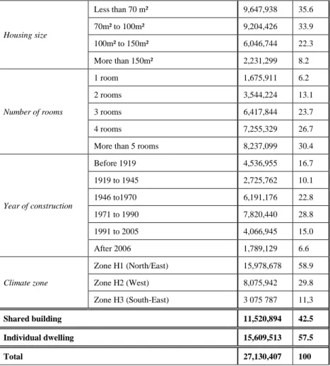
the second part is a survey of the dwelling’s energy performance conducted by a qualified professional. The EPD is provided free of charge to the respondent at the end of the survey and is valid for 10 years. In terms of survey scope, the statistical unit is the household’s principal residence. Responses relate to the dwelling’s energy performance and the household’s behavior. The dwelling sample is drawn from the French National Institute for Statistical and Economic Studies master sample for the 2011 annual census. The basic random sample is based on a complex multistage sampling design, and is representative of French regions, climatic zones, housing type and year of construction (some 27 million housing units). The EPD sample used for the present study includes 2,356 households. Table 2 provides more information on the French housing stock.
Table 2 - Distribution of French housing stock
Housing size Less than 70 m² 9,647,938 35.6 70m² to 100m² 9,204,426 33.9 100m² to 150m² 6,046,744 22.3 More than 150m² 2,231,299 8.2 Number of rooms 1 room 1,675,911 6.2 2 rooms 3,544,224 13.1 3 rooms 6,417,844 23.7 4 rooms 7,255,329 26.7
More than 5 rooms 8,237,099 30.4
Year of construction Before 1919 4,536,955 16.7 1919 to 1945 2,725,762 10.1 1946 to1970 6,191,176 22.8 1971 to 1990 7,820,440 28.8 1991 to 2005 4,066,945 15.0 After 2006 1,789,129 6.6 Climate zone Zone H1 (North/East) 15,978,678 58.9 Zone H2 (West) 8,075,942 29.8 Zone H3 (South-East) 3 075 787 11,3 Shared building 11,520,894 42.5 Individual dwelling 15,609,513 57.5 Total 27,130,407 100
Such rich, representative, interesting and detailed data are rare. The PHEBUS survey allows a detailed overview of primary residential units and their energy performance. The variables included in the survey include occupants’ socio-demographic attributes, technical aspects of the housing unit, household energy use and behavior, home appliances, energy type(s) and related consumption. It provides information on the dwelling’s energy performance based on the expert diagnosis. It is the first source of data on observed and theoretical household energy consumption in France. Table 3 presents summary statistics of the variables used in the econometric model.
Table 3
List and description of model variables
Variable Categories Frequency / Mean ST. Dev Min Max Household socio-economic attributes
Household income (€) 35,593 25171.72 8429 141033
Energy price (€/kWh) 0.15 0.096 0.063 0.256
Age of HRP (Household Responsible Person) 54 15.29 19 93
Number of household members (NHM) 2.55 1.27 1 9
Tenure type (TT) Owner 76.15
Rented 23.85
Dwelling characteristics
Dwelling efficiency (1/energy intensity) 0.046 0.028 0.0069 0.44
Total square footage (TSF) 92 51.41 27 250
Housing type Detached
individual dwelling 50.11 Shared building 49.89
Heating system (HS) Shared central 9.69
Individual central
76.97
Household behaviors
Equipment rate (number of pieces of electrical equipment)
6,61 2.971 1 23
Heating temperature 21.44 7.938 8 30
Lower heating in bedrooms(Reduced heating when housing unit is empty)
Yes 68.33
No 31.67
3.2. Modeling approach
3.2.1. Theoretical and methodological aspects
As already described, examining residential energy consumption is a complex issue involving numerous inter-related aspects such as the housing unit’s physical characteristics, its occupants’ attributes, lifestyles and behavior, type of heating system and appliances, climate conditions, energy prices, etc. Several papers study the nature and measurement of the rebound effect (Sorrell, 2007; Wu et al., 2016) using various approaches and estimation techniques including instrumental variables and ordinary least squares (OLS).
As well as measuring the rebound effect, we want to identify the main drivers of household energy consumption. We conduct cross-section analysis to measure the magnitude of the direct rebound effect on domestic energy consumption. In contrast to previous cross-section studies which mainly using OLS regression, we use quantile regression to assess the impact of energy price and dwelling efficiency for different levels of electricity use. The proposed model allows separate analysis of the effect of energy efficiency and fuel price on household electricity demand response. Further, the proposed quantile model helps to differentiate the effects of several variables on the entire consumption distribution.
Following Berkhout et al. (2000) and Sorrell and Dimitropoulos (2008), we define the rebound effect as the energy efficiency elasticity of energy services consumption i.e. “the proportionate
(percentage) change in energy consumption following a proportionate change in energy efficiency, holding the other measured variables constant” (Galvin, 2015).
𝜂𝜀(𝑆) =𝜕 𝑆 𝑆 / 𝜕 𝜀 𝜀 = 𝜕 𝑆 𝜕 𝜀 / 𝑆 𝜀 (1) where S is energy services consumption and ε is energy efficiency.
Energy services represent the benefits to the household from using energy. S can be measured as: 𝑆 = 𝜀 ∗ 𝐸 (2) (Galvin, 2015)
where E is the household’s energy demand.
Substituting eq. (2) for eq. (1) and using the product rule (Galvin, 2015), the rebound effect in terms of the energy efficiency elasticity can be described as:
𝜂𝜀(𝑆) = 1 +𝜕𝐸 𝜕𝜀 /
𝜀
𝐸 (3)
Note that taken together eqs. (1) and (3) comprise an identity that allows us to derive the following relationship between energy services demand and energy efficiency elasticities: 𝜂𝜀(𝐸) = 𝜂𝜀(𝑆) − 1 (4)
However, estimating dwelling energy efficiency corresponding to demand for domestic energy is complex. In broad terms, in France it can be defined as the amount of energy required to achieve comfortable indoor conditions in all of the rooms in the housing unit, in kWh of energy per square meter per year (kWh/m²/year). It can be written as:
𝜀 = 𝑘 𝐷⁄ (5)
where D is energy intensity and k is a constant. According to eqs. (1) and (4) ε is only ever used in rebound effect calculations as the denominator of ∂ε (or vice versa). Accordingly, it is not necessary to define a value for k because it is canceled out in this calculation (Galvin,
2015). Following Galvin’s (2015) approach, in this paper the value of ε can be expressed as: 𝜀 = 1 𝐷⁄ (6)
Substituting eq. (5) into eq. (2) allows a conceptual understanding of the notion of energy services: 𝑆 = 𝐸 𝐷⁄
Rather than using 𝜂𝜀(𝐸) and 𝜂𝜀(𝑆), several authors use the estimated price elasticity to proxy for the magnitude of the rebound effect (Berkhout et al., 2000; Haas and Biermayr, 2000; Sorell et al., 2009). Under specific assumptions, the rebound effect can be estimated using the own price elasticity (Sorell and Dimitropoulos, 2008). Hence, the rebound effect can be expressed formally as:
𝜂𝜀(𝐸) = − 𝜂𝑃𝑒(𝐸) − 1 (7) where, 𝑃𝑒 is the energy price.
In part, the choice of elasticity measure to proxy for the rebound effect depends on data availability. Data on energy prices and energy consumption are more readily available and more accurate than data on energy efficiency and energy services (Sorell et al., 2009). As already mentioned, here we use an efficiency and price elasticities theoretical framework to estimate the magnitude of the direct rebound effect related to residential electricity demand in France.
3.2.2. Model specification
Most studies of the direct rebound effect related to demand for energy that use micro-level individual data start with OLS where the variable coefficients are the conditional means of the model parameters. Conditional means can capture how consumers change their energy use with respect to changes in energy prices in general but provide only limited information on
the energy use behavior of consumers who consume more or less energy than the average consumer.
It is clear that energy demand is not homogeneous among households; households have different priorities, needs and preference for energy services. Therefore, an OLS regression technique based on conditional means is not appropriate to differentiate the rebound effect with respect to energy demand distribution across households. In addition, policies to mitigate the rebound effect based only on average effects are not elaborate and might be irrelevant. To formulate effective energy policy requires a good understanding of the energy use behavior of households in the tails of the energy demand distribution.
To explore the distributional rather than the average effects of household energy use behavior, we develop a bottom-up statistical approach based on a quantile regression model. Quantile regression parameters estimate the impact of the individual explanatory variables on a specific quantile (e.g. 10th, 25th, 50th, 75th) of the dependent variable.
Quantile regression was introduced by Koenker and Basset (1978) and developed by Koenker and Hallock (2001), and expands the concept of univariate quantile estimation to estimation of the conditional quantile functions based on one or more covariates.
In our study, the standard log-linear demand equation used to estimate the magnitude of the rebound effect can be written as:
𝑦𝑖 = 𝑥𝑖′𝛽 + 𝑢𝑖 (8)
Using OLS regression, estimation of the parameter coefficients can be written as:
min
𝛽∈𝑅𝑘∑(𝑦𝑖− 𝑥𝑖
′𝛽)2 (9) 𝑛
where 𝑦𝑖 is the vector of household electricity demand (in logarithm), x is a vector of all the regressors, 𝛽 is the vector parameters to be estimated and 𝑢𝑖 is a vector of the residuals. While the OLS model estimates the conditional mean, quantile regression estimates the conditional quantiles.
We suppose 𝜃 is a number ranging between 0 and 1, and the 𝜃𝑡ℎ quantile of the distribution of the distribution of electricity consumption y is denoted Q (𝜃). Q (𝜃) can be given by sorting the y values from smallest to largest. In the case of the quantile regression model, the vector of the 𝛽 parameters can be estimated for any quantile 𝜃 by minimizing the following function with respect to 𝛽 (Koenker and Basset (1978):
min
𝛽∈𝑅𝑘∑ 𝜃(𝑦𝑖 − 𝑥𝑖
′𝛽)2 𝜃 ∈ [0, 1] (10) 𝑛
1
The general 𝜃𝑡ℎ sample statistics quantile Q (𝜃) solves the following equation:
min 𝛽∈𝑅𝑘 ∑ 𝜃|𝑦𝑖 − 𝑥𝑖 ′𝛽| + ∑ (1 − 𝜃)|𝑦 𝑖 − 𝑥𝑖′𝛽| (11) 𝑛 𝑖∈〈𝑖:𝑦𝑖<𝑥𝑖𝛽〉 𝑛 𝑖∈〈𝑖:𝑦𝑖≥𝑥𝑖𝛽〉
The parameter vectors of 𝛽 for a given 𝜃 can be estimated using a linear programing algorithm.
𝛽̂𝜃 the estimator of the 𝜃𝑡ℎ quantile regression minimizes over the objective function below (Cameron and Trivedi, 2013):
min1 𝑛 𝛽 { ∑ 𝜃|𝑦𝑖 − 𝑥𝑖′𝛽𝜃| 𝑖:𝑦𝑖≥𝑥𝑖′𝛽 + ∑ (1 − 𝜃)|𝑦𝑖 − 𝑥𝑖′𝛽𝜃| 𝑖:𝑦𝑖<𝑥𝑖′𝛽 } = min1 𝑛 𝛽 ∑ 𝜑𝜃(𝑢𝜃𝑖) 𝑛 1 (12)
Using quantile rather than OLS regression has two major advantages. First, since household energy consumption is heterogeneous, a quantile approach allows inferences with respect to the effect of the explanatory factors conditional on the level of energy consumed. When the degree of data variation is important, quantile regression is the better strategy. The quantile regression parameters assess the variation in a specified quantile of household energy expenditure in response to a one-unit variation in the explanatory variable. Second, rather than assuming normality of the error terms conditional on the repressors, no assumptions are made about the distribution of the error term. Thus, quantile regression estimates are more flexible and more robust than OLS model estimates.
4. Results and discussion
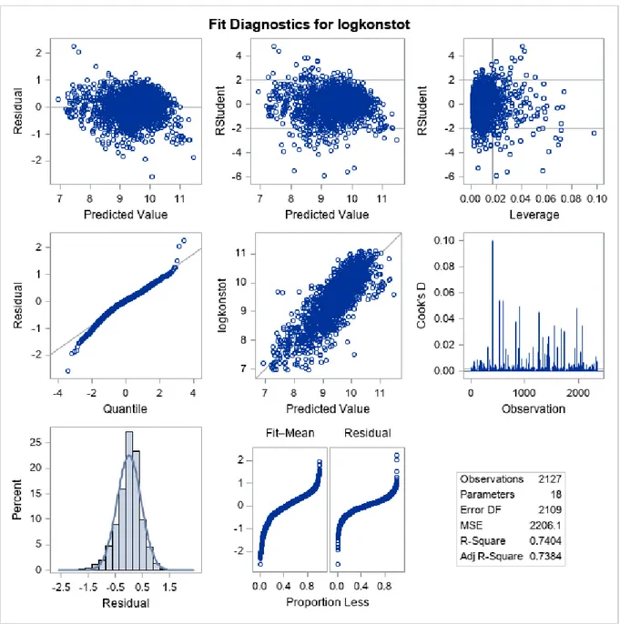
The empirical results of the quantile and OLS regressions are presented in table 6 and figs. 3a, 3b, 3c and 3d which depict the conditional quantile estimates of energy demand (dependent variable). Table 4 displays the results of the inference analysis of the OLS model including the F test. The charts in annex 2 provide the OLS model fit diagnostics, including residuals normality and heteroskedasticity.
Using OLS, the adjusted R² statistic is equal to 0.73 which is relatively high given that the dependent variable is estimated in share form. In addition, most of the control factor coefficients used in the model are statistically significant at the 1% level. Table 5 presents the Variance Inflation Factor (VIF) test results. The VIF values of all the variable are lower than 5 indicating that our models do not suffer from autocorrelation.
Table 4 Inference of the OLS model results
Table 5
Variance inflation factor test results
Variable GVIF DF GVIF^(1/(2*Df))
Energy price 1.517351 1 1.231808
Dwelling efficiency 1.299312 1 1.139874
Household income 1.582379 1 1.257927
Age of Household Responsible Person (HRP) 1.499666 1 1.224608
Number of household members 3.604374 1 1.898519
Owner occupier 1.453091 1 1.205442
Total square footage 1.981885 1 1.407794
Heating type 2.336258 2 1.236318
Multi-unit housing, flat 2.027012 1 1.423732
Equipment rate 2.469688 1 1.571524
Heating temperature 1.045989 1 1.022736
Heating degree days (HDD) 1.121973 1 1.059232
Note: GVIF denotes Generalized variance inflation factor Source Degree of
Freedom
Sum of Squares
Mean Square Fisher Value Pr > F Model 17 13272586.69 780740.39 353.91 <.0001 Error 2109 4652587.46 2206.06 Corrected Total 2126 17925174.14 R-Square Ajustedd-R² Coefficient Variation
Root MSE Number of observations
Table 6
Estimation results using quantile and OLS regression.
Dependent variable (Total electricity consumption)
Variable Q 0.1 Q 0.25 Q 0.5 Q 0.75 Q 0.9 OLS Energy price T statistics P value -0.38*** (-11,79) (<.0001) -0.44*** (-10,02) (<.0001) -0.57*** (-5,25) (<.0001) -0.65*** (-3,97) (<.0001) -0.71*** (-4,75) (<.0001) -0.45*** (-11.93) (<.0001) Dwelling efficiency -0.22** (-2.49) (0.0129) -0.27*** (-3.83) (0.0001) -0.28*** (-5.07) (<.0001) -0.20*** (-3.29) (0.0011) -0.14*** (-2.83) (0.0072) -0.24*** (-5.94) (<.0001) Household income 0.01 (-0.63) (0.5304) 0.02 (-0.24) (0.809) 0.05 (1.08) (0.2783) 0.03 (-0.55) (0.5806) 0.05 (-0.61) (0.5411) 0.01* (0.27) (0.7909) Age of HRP 0.02 (-0.11) (0.9155) 0.15* (1.53) (0.1274) 0.22** (2.32) (0.0205) 0.16* (1.73) (0.0638) 0.13 (1.12) (0.2652) 0.13** (2.32) (0.0206) Number of household members 0.12** (1.97) (0.0487) 0.18*** (4.65) (<.0001) 0.14*** (3.87) (<.0001) 0.16*** (3.96) (<.0001) 0.12** (2.41) (0.016) 0.14*** (5.49) (<.0001) Owner 0.11 (1.18) (0.2383) 0.05 (0.78) (0.4342) -0.09 (-1.54) (0.125) -0.17*** (-2.85) (0.0045) -0.11 (-1.46) (0.1453) -0.07 (-1.52) (0.1296)
Total square footage 0.44***
(4.13) (<.0001) 0.43*** (4.68) (<.0001) 0.49*** (5.43) (<.0001) 0.46*** (6.66) (<.0001) 0.50*** (4.44) (<.0001) 0.46*** (8.94) (<.0001) Shared central heating -0.25 (-0.18) (0.8556) -0.41 (-1.43) (0.1526) -0.26 (-0.94) (0.3482) -0.25 (-0.5) (0.614) -0.10 (-0.1) (0.9219) -0.37*** (8.94) (<.0001) Individual central heating -0.47*** (-3.67) (0.0003) -0.37*** (-5.08) (<.0001) -0.22** (-2.49) (0.0131) -0.22** (-1.98) (0.0481) -0.28** (-2.95) (0.0032) -0.36* (-1.90) (0.0575) Multi-unit housing, flat -0.14 (-1.21) (0.2268) -0.17** (-2.39) (0.0173) -0.21*** (-2.97) (0.0031) -0.25*** (-3.28) (0.0011) -0.22** (-1.96) (0.050) -0.21*** (-4.31) (<.0001) Equipment Rate 0.08 (0.67) (0.5052) 0.19** (1.87) (0.0617) 0.14 (1.52) (0.1277) 0.25*** (3.05) (0.0023) -0.23*** (1.97) (0.0495) 0.17*** (3.04) (<.0001) Heating temperature 0.09 (0.26) (0.7946) 0.33 (0.98) (0.3276) 0.46* (1.77) (0.0766) 0.49 (1.44) (0.1517) 0.06 (0.14) (0.8899) 0.48*** (2.48) (0.0132)
Heating degree days
(HDD) 0.14 (0.61) (0.545) 0.13 (0.82) (0.4119) 0.19* (1.76) (0.0713) 0.20* (1.75) (0.0808) 0.01 (-0.08) (0.9362) 0.15* (1.84) (0.0661)
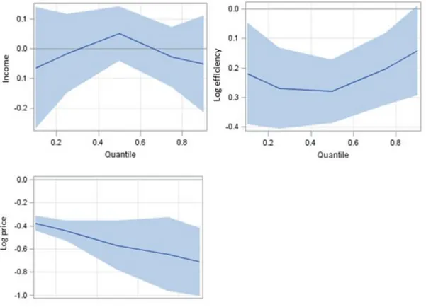
In the OLS model, the rebound effects due respectively to the price effect and the dwelling energy efficiency effect are around 45% and 76%. Obviously, OLS regression does not capture the price and energy efficiency effects on energy consumption for those households in the lower and upper tails of the consumption distribution. Nevertheless, the rebound effect estimates of the quantile regression suggest that households react differently to energy prices and dwelling energy efficiency along various quantiles of the conditional distribution. This can be explained by the different household energy uses, needs, habits and preferences. Figs. 3a and 3b depict the variations in the rebound effect due to price and dwelling efficiency effects with respect to the household electricity demand distribution. The upward sloping line in the positive quadrant in figs. X, y, z indicates that the impact of the focal variable is smaller in the lower than in the upper quantiles. The U-shape in the negative quadrants suggests that the effect is greatest in the middle of the distribution. A horizontal line would suggest that OLS estimates are sufficient.
First, our results confirm the existence of the price rebound effect and its sensitivity to group variations. This is the variation in the rebound effect due to the price effect with respect to the household energy demand distribution. Households whose energy demand is in the 10th quantile experience the lowest rebound effect - about 38%, while households whose electricity demand is in the 90th quantile experience the highest rebound effect - around 71%. For households whose energy demand is in the 25th, 50th, and 75th quantiles, the respective estimated rebound effects are 44%, 57% and 65%. This shows that there are large inequalities among households in relation to environmental deterioration and daily energy consumption (Berthe and Elie, 2015; Davis and Metcalf, 2016). Our results confirm previous work on the
sensitivity of the rebound effect to consumer group variations (Small and Dender, 2007; Gillingham, 2011). Looking at the heterogeneity in the price elasticity of the VMT (vehicle miles traveled) demand, West’s (2004) estimates confirm a U-shaped pattern of responsiveness. A possible explanation for this pattern is that budget constraints may be tighter at the low end, and the marginal utility of additional driving, may be lower at the higher end. Small and Dender (2007) assess the rebound effect for motor vehicles and find that the response to fuel price depends on the evolution of incomes and fuel costs. Similarly, Gillingham (2011) examines consumer heterogeneity and responsiveness to changes in the gas price, and highlights significant variation in responsiveness. Gillingham’s (2011) analysis provides suggestive evidence that heterogeneity in responsiveness among driver types is based on income, vehicle characteristics, driver demographics and geography. The recent study by Kulmer and Seebauer (2019) emphasizes the relevance of household heterogeneity for estimation of the rebound effect of energy efficiency improvements, and shows that the direct rebound effect is related significantly to heterogeneity among household groups. This result has implications for policymakers interested in more than just the aggregate response to energy efficiency and suggests the need for smart policies which take account of heterogeneity in consumer preferences.
Second, our results provide evidence of a substantial energy efficiency rebound effect with variation among groups of consumers. This variation is due to the energy efficiency effect with respect to the household energy demand distribution. Our results provide evidence of a rebound effect ranging between 72% and 86%. Households whose energy consumption
is in the 90th quantile experience the highest rebound effect - about 86%, while households whose energy demand is in the 50th quantile experience the lowest rebound effect - around 72%. Variation among groups of consumers in terms of the energy efficiency rebound effect may be explained by socio-economic factors and attitudinal factors. Previous research on green consumer behavior focuses mostly on curtailment behavior and energy efficiency behaviors as the main ways to reduce environmental damage and daily energy consumption (Testa et al., 2016; Karlin et al., 2014; Jansson et al., 2010). Efficiency behavior which is rooted in consumption habits is based on the adoption of technological solutions and requires some investment in information search and education. Burlinson et al. (2018 b) provide evidence of huge inequalities based on the difficulties experienced by low income households when investing in energy efficient technology. Understanding the reasons for adoption or non-adoption of new technologies would increase our understanding of citizens’ motives and expectations, their profiles, attitudes and pre-disposition towards technological innovations as well as the inequalities among households (Chester, 2014; Burlinson et al., 2018 a). Moreover, those in the first quantile who might have benefited more from energy efficiency will suffer a rebound effect due to possible increased in welfare and comfort which prevents their obtaining the full benefit of dwelling efficiency (Chan and Gillingham 2015; Fillipini et al., 2018). Those households that reduce their heating are in the intermediate (50th) quantile. The lowest quantile seems unable to take any actions while the households in the highest quantile seem to be reluctant to attend to this issue.
Third, our results show that in all quantiles the energy efficiency rebound effect is more pronounced and higher than the energy price rebound effect. While most of the economic literature uses energy price to estimate the rebound effect, our results suggest that if the data allow energy efficiency is a better measure. Our findings have several explanations. First, the rebound effect estimated by energy price supposes that consumers act symmetrically to a price increase or decrease. However, this does not apply in our case if we examine the behavior of different quantiles. The value of the savings resulting from a decrease of energy price differs for different quantiles. Second, the rebound effect based on the energy price is calculated using theoretical not current (real) prices. Our findings confirm the intuition in Chan and Gillingham (2015) that demand for services and price elasticities capture essentially distinct implicit price changes compared to service prices and efficiency elasticities of demand for services. Therefore, estimates of the rebound effect based on the first two elasticities may be biased. Our alternative strategy shows that the rebound effect and the differences between quantiles are more pronounced. In addition, and in relation to the French context, some scholars find that the type of tariff does not create a proper incentive for reducing energy consumption (Salies, 2013). If tariffs are meaningful to and properly understood by consumers they can act as a kind of extrinsic motivation and provide significant incentives and promote behavioral changes (Baum and Gross, 2017).
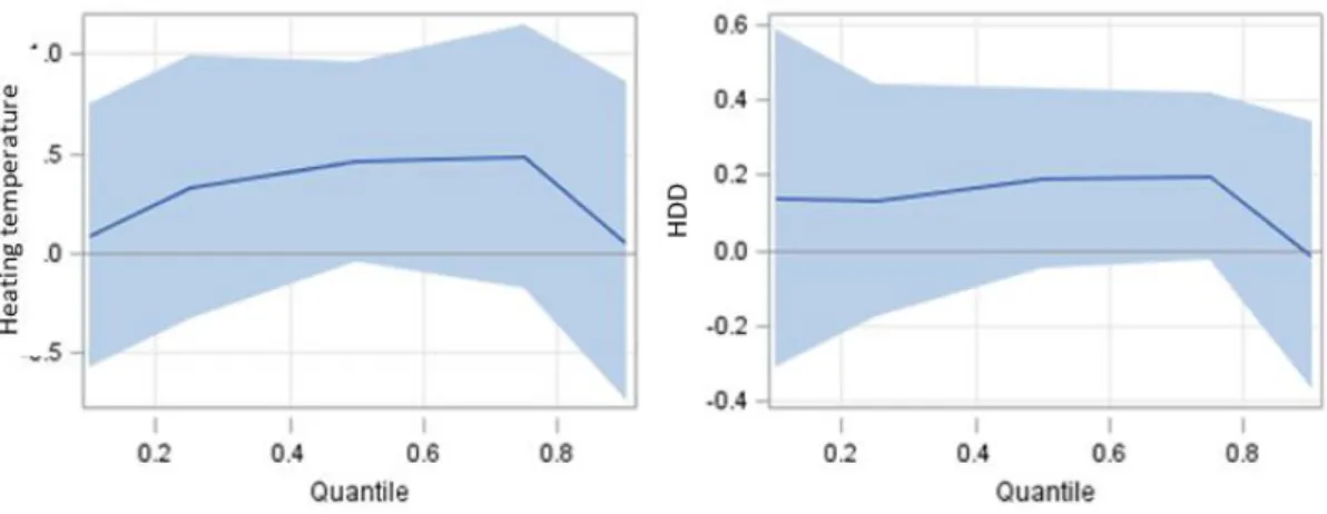
Fourth, the rebound effect calculated based on dwelling efficiency shows a non-linear relationship. Fig 3b shows that the lowest rebound effect occurs in the 5th quantile and is most pronounced in the 9th quantile. This non-linearity does not apply to the energy price rebound effect calculation. This result implies that there are other sociological and
psychological factors in addition to revenue that need to be considered in debates on energy efficiency. Consumption patterns and consumer behaviour are complex and are not captured only by revenue differences. Energy savings based on “efficiency behavior” in the form of purchase of more efficient appliances or investment in structural changes to the home might be less acceptable than “curtailment behaviors” related to reducing energy use which costs less and requires minimal changes to habitual actions (Karlin et al., 2014). Indeed “exclusive reliance on self-interest to foster energy conservation- while ignoring the more intrinsic reasons for acting environmentally- can backfire and diminish the likelihood that behavioral change even takes place” (Baum and Gross, 2017, p.71).
Fifth, our results suggest the need for specific attention to the energy efficiency behaviour of the lowest quantiles. Over the last two decades, debate on energy poverty shows that the poor are deprived of energy consumption. This deprivation can lead to underinvestment in human capital and inter-generational poverty. As the relative price of energy decreases with energy efficiency, impoverished households may be able to catch-up and increase their consumption of energy. Any policy directed to reducing energy consumption should consider social inequality and take care not to increase social vulnerability and discrimination among groups of households (for an illustration of increased energy poverty in the Chilean context see Reyes et al., 2019).
Sixth, our results on differences in the size and composition of the rebound effect may be linked to the nature of the commodity. Energy is perceived by households as an invisible commodity (Hargreaves et al., 2010; Maréchal, 2010) which results in lack of awareness about
its consumption especially among French consumers (Kendel et al., 2017). These historical conditions are critical for understanding the influence of social frames, and particularly representation of energy problems for French households (see Chester and Elliot, 2019, for a similar discussion related to Australia).
In France and in Europe generally, households are poorly informed about their electricity use, and have no control over its price. Several studies show that the information provided on electricity bills does not allow consumers to plan behavior changes, or link a reduction in their consumption to their equipment or habits (Wall and Crosbie, 2009). Lack of this information could affect decisions about consumption practices and environmental considerations (Bartiaux, 2008; Halkier, 2001). Mental compartmentalization allows some consumers to keep “green reflections out of certain practices” (Halkier, 2001, p.39), and to exhibit a kind of self-defense against daily green practices and decisions that might interfere with everyday comfort and convenience (Shove, 2003; Lynas, 2007). “Mental zapping” can divert households’ attention from the need to reduce energy consumption through significant changes to daily life (Sweeney et al., 2013). To investigate the rebound effect requires consideration of behavioral spillovers (Baum and Gross, 2017). Focusing only on the benefits of behavioral change in a single domain is not sufficient to capture its full significance but only whether it results in reduced consumption.
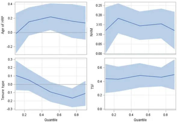
We not that most our control variables are significant. We notice that for some variables such as number of household members and housing size quantile regression does not add much more information than OLS. However, this does not apply to age of household responsible person, house ownership or heating type. Quantile regression captures variation
among quantiles and shows that most effects are not linear. The rebound effect linked to energy efficiency is non-linear and is more pronounced in the extreme quantiles. This is an important novelty of our analysis.
Finally, our results highlight the difficulties involved in obtaining accurate estimates of the rebound effect.While the basic mechanisms of the rebound effect are widely accepted, its magnitude and importance are disputed (Sorrell and Dimitropoulos, 2008; Thomas and Azevedo, 2013; Chan and Gillingham; 2015, Zhang et al., 2017). So far, existing studies employ distinct definitions of the dependent and independent variables, apply different estimation strategies and controls and focus on different energy services. In addition, this body of work is too limited and diverse to allow a coherent approach to this problem. The majority of previous quantitative studies on the rebound effect analyze price-induced rebounds due mainly to lack of data on energy efficiency. However, rebound effect estimates based on this methodology fluctuate among distinct end-uses, energy services, sectors, levels of aggregation and countries (Berkhout et al., 2000; Sorrell and Dimitropoulos, 2008). Empirical studies using prices elasticities are subject to bias, shows larger magnitudes over the long-run compared to the short run, and magnitudes that increase proportionately with the energy price level. Further, Chan and Gillingham (2015) highlight that demand for services and price elasticities capture essentially distinct implicit price changes compared to service prices and efficiency elasticities of demand for services. However, Sorrell and Dimitropoulos (2008) argue that most existing empirical analyses of the direct rebound effect rely on price-elasticities and use mainly upon cross-section or historical energy prices. They suggest that such estimates could overestimate the magnitude of the rebound effect for various reasons
including (i) price elasticity asymmetry, (ii) the expected positive correlation between other groups of input costs mainly capital costs and energy efficiency, (iii) the role of price induced efficiency enhancements, (v) the expected negative correlation between time efficiency and energy efficiency, and (vi) energy efficiency endogeneity. This ongoing debate indicates the lack of methodologically diverse analyses. We underline the need for more studies in this direction. Although availability of detailed individual data constitutes a constraint, it should be possible to use data on a wider range of goods (e.g. food and beverages) and energy services (e.g. appliances, lighting, etc.), and employ more innovative, quasi-experimental approaches.
Fig. 3.b. Estimated parameter by quantile with 95% confidence limits
5. Conclusion
Energy policymakers tend to focus on improving energy efficiency in the residential sector to reduce demand for energy. However, due to the rebound effect which leads to lower savings than expected when energy efficiency increases, investments in energy efficiency may not yield the expected energy savings. Understanding the rebound effect and measuring its magnitude are prerequisites for energy policy formulation. While an increasing number of studies investigate residential energy efficiency, few provide empirical examinations of the magnitude of the rebound effect on residential electricity demand. Also, studies of the rebound effect use a variety of measures which are affected by technical bias and poor-quality data. Most estimate the rebound effect based on elasticity of the demand price and previous prices, and find a large rebound effect (Sorrell et al., 2009). Our study employs robust estimation methods based on recent and original individual data.
Using a quantile regression approach and micro-level data from the French 2013 PHEBUS survey, we estimated the magnitude of the direct rebound effect on residential electricity consumption in France. Our empirical results show the existence of a substantial direct effect ranging between 38% and 86% (38%-71% using price elasticity, and 72%-86% using efficiency elasticity), and heterogeneity among consumption quantiles. They confirm previous work on the sensitivity of the rebound effect to consumer group variation. Our findings reject the hypothesis of a backfire effect in the context of residential electricity consumption in France. They suggest the need for policy to include carbon taxation, energy efficiency and alternative energy to facilitate France’s transition to a low-carbon economy. The findings confirm a direct rebound effect for residential electricity consumption by linking electricity
demand to energy prices, housing energy efficiency, type and number of household occupants and dwelling type. This should allow more tailored, effective and energy efficiency strategies. Our results show that considering different segments of the population could be beneficial since it is likely that individuals will exhibit different levels of energy use depending on their personal profiles.
From a public policy perspective, we would stress that promoting energy efficiency and use of energy efficient technology in buildings would provide benefits to many different stakeholders. These benefits would include energy savings, reduced Greenhouse Gas (GHG) emissions, energy security, reduced fuel poverty, improved health and well-being (improved indoor air quality), improved quality and durability of housing stock, increasing property values and more employment in the green sector. The building sector could play an important part in achievement of sustainable energy. Existing buildings are responsible for over 40% of the world’s total primary energy consumption and account for 24% of world CO2 emissions. Yet, despite the proven cost-effectiveness of reducing energy consumption through energy-efficient technologies, a large portion of the potential in the existing residential building sector remains untapped. Together with other authors (Vassileva et al., 2012; Podgornik et al., 2016), we think that targeting specific segments of the population is critical. As underlined by Vassileva and Campillo (2014), although low-income households tend to use less energy, they simultaneously have a greater interest in learning how to save energy and reduce their bills. An interesting direction for future energy-efficiency programs could be to target diverse groups of low and high levels of energy consumption to observe their different capacity for changing behavior and different levels of involvement in the issue.
There needs to be a policy shift from technically oriented efficiency programs towards a mix of technological and behavioral change. To achieve higher levels of energy savings, government should implement a policy package which includes support for improving the energy efficiency of existing dwellings, flexibility within existing regulatory frameworks, help for occupants to improve the energy efficiency of their housing units, energy rating and certification schemes, information on financing options, etc.
From a policy perspective, our paper has several implications. First, since our paper shows that energy efficiency and behavior vary among quantiles, there is a need to refine existing policies based on the homogeneous behavior of the population. This is crucial for the design of targeted policy interventions allowing measures oriented to specific groups, particularly households in the tails of the energy demand distribution. While France has implemented energy efficiency policies for several decades, few of these policies are based on differentiation among quantiles and sub-groups. Second, the behavior of the lowest quantiles may be explained by previous deprivation among poor households. Since energy efficiency savings lower the relative price of energy and induce an increase in consumption previous deprivation has an impact on behavior, especially due to the specificity of energy. Most economists agree on the importance of addressing fuel vulnerability and the negative impacts of cold homes, and improving the quality of life of many households by making their homes warmer and more efficient. Therefore, rather than seeing the rebound effect as a deterrent to energy efficiency policies, energy policymakers should incorporate welfare benefits and losses in their evaluations.
Third, our paper provides information on the part played by occupants’ behavioral and attitudinal factors in shaping residential demand for electricity in France. In this case, a holistic approach is required which integrates complex household behaviors and captures the drivers of energy efficiency. This would allow better assessment of energy-saving policy schemes. Finally, energy policymakers may not be able to influence objective contextual factors faced by consumers; however, they should design policies to leverage consumer attitudes and perceptions. Understanding the factors influencing energy-saving behaviors is crucial for achieving significant reductions in residential energy consumption. It would allow design and implementation of more effective intervention strategies to promote occupant energy-saving behaviors. To induce behavioral changes, occupants need the capability, knowledge, and intrinsic and extrinsic motivation and opportunities for implementing change. There are several intervention strategies that might encourage energy-saving behaviors among occupants, including (i) information and education (e.g. workshops to increase energy knowledge and to give some opportunity to change habits), (ii) goal setting and feedback (e.g. assigning an energy reduction target, and giving feedback to households to measure progress and increase extrinsic motivation), (iii) persuasion (e.g. using communication to induce positive and intrinsic motivation towards energy reduction and environmental action), (iv) incentives (e.g. fiscal incentives and monetary rewards for those on the lowest incomes), (v) empowerment (e.g. examples that occupants could aspire to or imitate) and (vi) enablement (e.g. increasing means and reducing barriers to increase capabilities and opportunities for households in the fuel poverty trap).
References
Antweiler, W., Gulati, S., 2016. Frugal Cars or Frugal Drivers? Sauder School of Business, University of British Columbia.
Azevedo, I.M., 2014. Consumer end-use energy efficiency and rebound effects. Annual Review of Environment and Resources, 39, 393-418.
Bartiaux, F., 2008. Does environmental information overcome practice compartmentalization and change consumers’ behaviours? Journal of Cleaner Production, 16, 1170-118.
Baum, C.M, Gross, C., 2017 .Sustainability policy as if people mattered: developing a framework for environmentally significant behavioral change. Journal of Bioeconomics, 19, 53- 95.
Belaïd, F., 2016. Understanding the spectrum of domestic energy consumption: Empirical evidence from France. Energy Policy, 92, 220-233.
Belaïd, F., 2017. Untangling the complexity of the direct and indirect determinants of the residential energy consumption in France: Quantitative analysis using a structural equation modeling approach. Energy Policy, 110, 246-256.
Belaïd, F., Garcia, T., 2016. Understanding the spectrum of residential energy-saving behaviours: French evidence using disaggregated data. Energy Economics, 57, 204-214.
Belaïd, F., Joumni, H., 2020. Behavioral attitudes towards energy saving: Empirical evidence from France. Energy Policy, 140, p.111406.
Belaïd, F., Bakaloglou, S., Roubaud, D., 2018. Direct rebound effect of residential gas demand: Empirical evidence from France. Energy Policy, 115, pp.23-31.
Berkhout, P. H., Muskens, J. C., Velthuijsen, J. W., 2000. Defining the rebound effect. Energy policy, 28(6), 425-432.
Berthe, A., Elie, L., 2015. Mechanisms explaining the impact of economic inequality on environmental deterioration. Ecological economics, 116,.191-200.
Binswanger, M., 2001., Technological progress and sustainable development: what about the rebound effect? Ecological economics, 36(1), 119-132.
Borenstein, S., 2015., A Microeconomic Framework for Evaluating Energy Efficiency Rebound and Some Implications. The Energy Journal, 36(1), 1-21.
Brookes, L. G., 1978. Energy policy, the energy price fallacy and the role of nuclear energy in the UK. Energy Policy, 6(2), 94-106.
Burlinson, A., Giulietti, M. Battisti, G., 2018 a. The elephant in the energy room: Establishing the nexus between housing poverty and fuel poverty. Energy Economics, 72, 135-144.
Burlinson, A., Giulietti, M., Battisti, G., 2018 b. Technology adoption, consumer inattention and heuristic decision-making: Evidence from a UK district heating scheme, Research Policy, 47(10), 1873-1886. Cameron, A. C., Trivedi, P. K., 2013. Regression analysis of count data (Vol. 53). Cambridge University Press. Chan, N. W., Gillingham, K., 2015. The microeconomic theory of the rebound effect and its welfare