HAL Id: cea-02408231
https://hal-cea.archives-ouvertes.fr/cea-02408231
Submitted on 12 Dec 2019
HAL is a multi-disciplinary open access
archive for the deposit and dissemination of
sci-entific research documents, whether they are
pub-lished or not. The documents may come from
teaching and research institutions in France or
abroad, or from public or private research centers.
L’archive ouverte pluridisciplinaire HAL, est
destinée au dépôt et à la diffusion de documents
scientifiques de niveau recherche, publiés ou non,
émanant des établissements d’enseignement et de
recherche français ou étrangers, des laboratoires
publics ou privés.
Laser Interferometer Space Antenna
C. Danielski, V. Korol, N. Tamanini, E. M. Rossi
To cite this version:
C. Danielski, V. Korol, N. Tamanini, E. M. Rossi. Circumbinary exoplanets and brown dwarfs with
the Laser Interferometer Space Antenna. Astronomy and Astrophysics - A&A, EDP Sciences, 2019,
632, pp.A113. �10.1051/0004-6361/201936729�. �cea-02408231�
Astronomy
&
Astrophysics
https://doi.org/10.1051/0004-6361/201936729© C. Danielski et al. 2019
Circumbinary exoplanets and brown dwarfs with the Laser
Interferometer Space Antenna
C. Danielski
1,2, V. Korol
3,4, N. Tamanini
5, and E. M. Rossi
31AIM, CEA, CNRS, Université Paris-Saclay, Université Paris Diderot, Sorbonne Paris Cité, 91191 Gif-sur-Yvette, France e-mail: camilla.danielski@cea.fr
2Institut d’Astrophysique de Paris, CNRS, UMR 7095, Sorbonne Université, 98 bis bd Arago, 75014 Paris, France 3Leiden Observatory, Leiden University, PO Box 9513, 2300 RA Leiden, The Netherlands
4School of Physics and Astronomy, University of Birmingham, Edgbaston, Birmingham B15 2TT, UK
5Max-Planck-Institut für Gravitationsphysik, Albert-Einstein-Institut, Am Mühlenberg 1, 14476 Potsdam-Golm, Germany Received 18 September 2019 / Accepted 11 October 2019
ABSTRACT
Aims. We explore the prospects for the detection of giant circumbinary exoplanets and brown dwarfs (BDs) orbiting Galactic double white dwarfs (DWDs) binaries with the Laser Interferometer Space Antenna (LISA).
Methods. By assuming an occurrence rate of 50%, motivated by white dwarf pollution observations, we built a Galactic synthetic population of P-type giant exoplanets and BDs orbiting DWDs. We carried this out by injecting different sub-stellar populations, with various mass and orbital separation characteristics, into the DWD population used in the LISA mission proposal. We then performed a Fisher matrix analysis to measure how many of these three-body systems show a periodic Doppler-shifted gravitational wave pertur-bation detectable by LISA.
Results. We report the number of circumbinary planets (CBPs) and BDs that can be detected by LISA for various combinations of mass and semi-major axis distributions. We identify pessimistic and optimistic scenarios corresponding, respectively, to 3 and 83 (14 and 2218) detections of CBPs (BDs), observed during the length of the nominal LISA mission. These detections are distributed all over the Galaxy following the underlying DWD distribution, and they are biased towards DWDs with higher LISA signal-to-noise ratio and shorter orbital period. Finally, we show that if LISA were to be extended for four more years, the number of systems detected will be more than doubled in both the optimistic and pessimistic scenarios.
Conclusions. Our results present promising prospects for the detection of post-main sequence exoplanets and BDs, showing that grav-itational waves can prove the existence of these populations over the totality of the Milky Way. Detections by LISA will deepen our knowledge on the life of exoplanets subsequent to the most extreme evolution phases of their hosts, clarifying whether new phases of planetary formation take place later in the life of the stars. Such a method is strongly complementary to electromagnetic studies within the solar region and opens a window into the investigation of planets and BDs everywhere in the entire Galaxy, and possibly even in nearby galaxies in the Local Group.
Key words. planets and satellites: detection – brown dwarfs – white dwarfs – gravitational waves – planets and satellites: gaseous planets
1. Introduction
In an epoch in which the field of exoplanets is moving at a fast pace and groundbreaking discoveries are made, very little is known about the ultimate fate of planetary systems. In the Milky Way more than ∼97% of the stars will turn into a white dwarf (WD), meaning that the vast majority of the more than known 3000 planet-hosting stars will end their life as WDs. Can their planets survive stellar evolution? Theoretical models indicate that a planet can endure the host-star evolution if it avoids engulfment or evaporation throughout the red giant or/and the asymptotic giant branch phases (e.g. Livio & Soker 1984;
Duncan & Lissauer 1998;Nelemans & Tauris 1998), where sur-vival itself depends, among various parameters, on the initial semi-major axis and planetary mass (Villaver & Livio 2007). For what remains of the planetary system the complex long-term orbital evolution, consequent to stellar evolution, may yield to planet ejections and/or collisions (e.g.Debes & Sigurdsson 2002;Veras et al. 2011;Veras 2016;Mustill et al. 2018). Besides, if migration or scattering occurs towards the proximity of the
Roche limit, strong tidal forces can further crush the planetary cores (Farihi et al. 2018), like in the case of the planetesimal found shattering around WD 1145+017 (Vanderburg et al. 2015). Such a fragmentation process consequently enables the forma-tion of a debris disc, made of metal-rich planetary material, which could in turn accrete onto the WD, polluting its atmo-sphere (e.g.Jura et al. 2009;Farihi et al. 2010;Farihi 2016;Veras 2016;Brown et al. 2017;Smallwood et al. 2018).
2. Evidences for sub-stellar objects around WDs 2.1. White dwarf pollution
White dwarfs are expected to have a pure H or He atmosphere (Schatzman 1945) and their high surface gravity (∼105 denser
than the Sun) makes the sinking metals diffusion timescale sev-eral order of magnitude shorter than the evolutionary period. Yet, observations show the presence of heavy elements in the spectra of 25–50% of all observed WDs (Zuckerman et al. 2003,
2010;Koester et al. 2014), indicating that a continuous supply of
A113, page 1 of15
metal-rich material accreting onto these stars must be present. There are several sources of WD pollution proposed in the litera-ture. This WD pollution could originate from planetary material (i.e. from circumstellar debris discs as previously explained), moons via planet–planet scattering (Payne et al. 2016, 2017), or comets (Caiazzo & Heyl 2017). It could also be from per-turbations created by eccentric high-mass planets, which drive substantial asteroids or minor bodies to the innermost orbital region around the star (which in some cases is within the stel-lar Roche limit), thereby yielding to tidal fragmentation (e.g.
Frewen & Hansen 2014;Chen et al. 2019;Wilson et al. 2019). The last source of WD pollution is currently preferred in the community. Pollution of WDs in wide binaries may also be caused by Kozai–Lidov instabilities, which can cause the orbit of objects such as planets, to intersect the tidal radius of the WD, causing their distruction (Hamers & Portegies Zwart 2016;
Petrovich & Muñoz 2017).
Overall WD pollution studies support the evidence of dynamically active planetary systems orbiting WDs. Nonethe-less, because of the intrinsic low luminosity of these stars, no planets have been detected yet around single WDs, but an intact planetesimal has been observed inside a debris disc belonging to a WD (Manser et al. 2019).
2.2. Generations of circumbinary post-common envelope exoplanets
Contrary to the single star case, P-type exoplanets (Dvorak 1986) have been detected orbiting binary stars in which the higher mass component has already grown to be a WD (i.e. the mass of its progenitor is M∗ . 10 M ); the second component is usually
a low-mass star that will become a giant later in its life (i.e. NN Ser, HU Aqr, RR Cae, UZ For, and DP Leo; Beuermann et al. 2010, 2011; Qian et al. 2011, 2010, 2012; Potter et al. 2011). These discoveries prove that planets can survive at least one common envelope (CE) phase, i.e. a shared stellar atmo-sphere phase typical of close binary stars, which happens when one of the binary components becomes a giant (see Sect. 3.1
for more detail on this phase). Surviving planets (in this case first generation planets) are usually called post-main sequence exoplanets or post-CE exoplanets, and they are more likely to survive around evolving close binary stars than around evolv-ing sevolv-ingle stars (Kostov et al. 2016). Only a small amount is known about these planets, but they are extremely interesting as they provide a link between planetary formation and fate, as well as constraints on tidal, binary mass loss, and radiative process (Veras 2016).
Detection and study of these bodies can also provide us with further information about planetary formation processes. There is the interesting hypothesis that some of these known post-CE planets belong to a “new generation”, i.e. they have formed after the first CE phase (e.g.Zorotovic & Schreiber 2013;Völschow et al. 2014). A study byKashi & Soker(2011) has shown that because of angular momentum conservation and further inter-action with the binary system, 1–10% of the ejected envelope does not reach the escape velocity. This material remains bound to the binary system, falls back on it, flattens, and forms a cir-cumbinary disc, which could provide the necessary environment for the formation of a second generation of massive exoplan-ets (Perets 2010; Völschow et al. 2014; Schleicher & Dreizler 2014). On the other hand, as already mentioned for the single star case, some sub-stellar bodies (e.g. first generation exoplan-ets, asteroids, and comets), whose orbit is small and/or eccentric enough, could be tidally disrupted during the CE phase, creating
a circumbinary disc of rocky debris, out of which new terrestrial exoplanets can grow (Farihi et al. 2017). In both cases photo-heating from the binary, photoionisation, radiation pressure, and differences in the magnetic field, would likely be responsible for influencing the discs in different ways, causing second genera-tion planets to differ from first generagenera-tion planets (Perets 2010;
Schleicher & Dreizler 2014;Veras 2016).
Another possibility is the existence of a hybrid generation: first generation planets that survive the first CE phase and may have been subject to mass loss throughout the whole process. Either way, the resulting planet/planetesimal could now accrete on the disc material, producing more massive planets on higher eccentricity (Armitage & Hansen 1999;Perets 2010). The out-come would be a planet with a first generation inner core and second generation outer layers. In this case the formation of a giant planet could be faster than for first generation giant planets. The same hypothesis is similarly applicable if the binary overgoes a second CE phase, i.e. the low-mass star overflows its Roche lobe and shares its atmosphere with the WD companion. After this stage we might have either a third generation of exo-planets forming around a double white dwarf (DWD) system, a hybrid generation, or previous surviving generations. To date no exoplanets are known orbiting a DWD (Tamanini & Danielski 2019), and the only circumbinary exoplanet known orbiting a system with two post-main sequence stars (i.e. a WD and a millisecond pulsar) is the giant PSR B1620-26AB b; this planet is also the first circumbinary exoplanet confirmed (Sigurdsson 1993; Thorsett et al. 1993). Because the planetary system PSR B1620-26AB is the result of a stellar encounter in the Milky Way plane (Sigurdsson et al. 2003), it is not directly representative of a standard (i.e. isolated) binary planetary system evolution.
Possibly because of an observational bias, all the post-CE planets discovered until now are giant planets with masses M ≥ 2.3 MJ and semi-major axes a ≥ 2.8 au. The most successful
technique used for their detection is eclipse timing variation (ETV), which is sensitive to wider planetary orbits and hence requires a long observational baseline to precisely time the eclipses. Also, ETV typically suffers from a lack of cross valida-tion and errors that are not uncommon, for example, the lack of accurate timing in the instrumentation used or procedures used to place the recorded times onto a uniform timescale corrected for light travel time (Marsh 2018). Any small inaccuracy or anal-ysis imprecision could lead to uncertainties in the validity of a planet in the system, with the planets potentially being the wrong interpretation of the Applegate mechanism (Applegate 1992).
RecentlyTamanini & Danielski 2019showed the possibility to detect Magrathea-like (Adams 1979) planets, i.e. circumbi-nary exoplanets orbiting DWDs by using the Laser Interferome-ter Space Antenna (LISA;Amaro-Seoane et al. 2017) to measure the characteristic periodic modulation in the gravitational wave (GW) signal produced by the DWD. Compared to the classic detection methods, the GW approach has the advantages that this method is (i) able to find exoplanets all over the Milky Way and in other close-by galaxies; (ii) not limited by the magnitude of the WDs, but on the parameters from which the GW depends (see Sect.3.3); and (iii) not affected by stellar activity, which is an issue reported in electromagnetic (EM) observations. 2.3. Brown dwarfs
Brown dwarfs (BDs) are by definition bodies that are not massive enough to fuse hydrogen in their interior stably, but are mas-sive enough to undergo a brief phase of deuterium burning soon
after their formation. The very first two BDs were discovered in 1995 (Nakajima et al. 1995; Rebolo et al. 1995), and today over 1000 BDs have been detected in the solar neighbour-hood (Burningham 2018). Some of these objects have also been discovered around single WDs. Examples of BDs orbiting at dis-tances beyond the tidal radius of the asymptotic giant branch progenitor, but also within it (e.g. WD 0137-349 B,Maxted et al. 2006), show that BDs can survive stellar evolution whether or not they are engulfed by their host’s envelope.Farihi et al.(2005) predicted that a few tenths of percent of Milky Way single WDs host a BD.
Concerning the binary case, the ETV technique allowed observers to detect a few post-CE systems with one evolved binary, comprised of a WD and a low-mass star, and a BD companion(s). Some examples of such systems are HQ Aqr, V471 Tau, HW Vir, and KIC 10 544 976 (Go´zdziewski et al. 2015;Vaccaro et al. 2015;Beuermann et al. 2012;Almeida et al. 2019). No BD has been found orbiting DWDs but, similar to the case of circumbinary planets (CBPs), if such a population exists, it could be found through GW astronomy with the LISA mission (Robson et al. 2018;Tamanini & Danielski 2019). As a matter of fact a BD, because it is more massive than a planet, would produce a stronger GW perturbation that is easier to detect with respect to a CBP.
Recalling the hypothesis of an hybrid generation (Sect.2.2), the core of a surviving body could efficiently accrete on the stellar ejecta disc, forming exceptionally massive planets which de facto become BDs (Perets 2010). In this case BDs would be able to form more often within the famous BD desert (Marcy & Butler 2000).
2.4. Detecting sub-stellar objects around binary WDs with LISA
The focus of this work is to follow up onTamanini & Danielski
(2019) and to quantitatively estimate the LISA detection rates of circumbinary exoplanets as well as circumbinary BDs. Brown dwarfs have masses ranging between the stellar and plane-tary domain; nevertheless, while the difference with stars is well defined, the separation with planets is still an open subject of discussion. The different nature of these objects could be either based on their intrinsic physical properties (Chabrier & Baraffe 2000) or on their formation mechanism (Whitworth et al. 2007). Furthermore, more recentlyHatzes & Rauer(2015) anal-ysed the density versus mass relationship for objects with mass ∼0.01 MJ < M < 0.08 M , and identified three distinct regions
that are separated by a change in slope in such a relation (at M = 0.3 MJ and M = 60 MJ). Above M = 60 MJ, but lower than
M = 0.08 M , the BDs domain, and below that limit (but above
M = 0.3 MJ) the giant planets domain.
Because of this ongoing discussion we hence decided to not limit our analysis to the mass domain reported in Tamanini & Danielski (2019), but to account for a larger mass range, up to the stellar limit. Consequently throughout this manuscript, for simplicity we define a sub-stellar object (SSO) to be a celestial body with mass less than 0.08 M (the hydrogen burning limit,
which includes the upper uncertainty byWhitworth 2018). This category is divided between CBPs and BDs. As inTamanini & Danielski(2019) we define the former as objects with mass M ≤ 13 MJ(the deuterium burning limit) and the latter as those with
mass 13 MJ< M < 0.08 M . For simplification only the mass
and no spectroscopic and/or formation mechanism classification are accounted for in this work.
The outline of this manuscript is as follows: in Sect. 3 we present the characteristics of populations used in the investiga-tion, and we summarise the GW detection method discussed in
Tamanini & Danielski(2019). In Sect. 4 we report CBPs and BDs detection rates, with their error analyses, for both the LISA nominal mission and for a possible extension of four more years. We discuss the implications of our results in Sect. 5 and we conclude in Sect.6.
3. Method
To reach the scope of this study we worked throughout two different stages. First, we constructed a population of Galac-tic detached DWDs with circumbinary exoplanets/BDs. To do so we injected a simulated population of SSOs into a synthetic population of DWDs (Korol et al. 2017). Such a DWD popula-tion was specifically designed to study the LISA detectability of these binary WDs, and it was employed in the LISA mission pro-posal (Amaro-Seoane et al. 2017). Second, we used the method described inTamanini & Danielski(2019) to measure how many SSOs LISA will be able to detect.
In Sect. 3.1 we summarise the most important features of the DWDs population. In Sect.3.2we provide details about the SSOs population injection process. In Sect.3.3we summarise the method used for the LISA GW detection of a circumbinary SSOs.
3.1. LISA DWD population
Our method relies on the binary population model whichToonen et al. (2012) obtained using binary population synthesis code SEBA, originally developed by Portegies Zwart & Verbunt
(1996) and later adapted for DWDs byNelemans et al.(2001b) andToonen et al.(2012). The progenitor population is initialised by randomly sampling initial distributions of binary properties with a Monte Carlo technique. Specifically, the mass of the pri-mary star is drawn from the Kroupa initial mass function in the range between 0.95 and 10 M (Kroupa et al. 1993). The mass
of the secondary star is derived from a uniform mass ratio dis-tribution between 0 and 1 (Duchêne & Kraus 2013). A log-flat distribution and a thermal distribution are adopted for the initial binary orbital separations and binary eccentricities, respectively (Abt 1983; Heggie 1975;Duchêne & Kraus 2013). The initial binary fraction is fixed to 0.5 value. The SEBA code evolves
binaries until both stars turn into WDs and beyond up to the present time. More details and discussion on the sensitivity of the binary population synthesis outcome to the aforementioned assumptions are given inToonen et al.(2012,2017). The adopted model has also been recently tested against observations of both single WDs and WDs in binary systems (including DWDs) in the solar neighbourhood byToonen et al.(2017). In particular, the adopted model currently better represents the space density of DWDs derived from a spectroscopically selected sample of
Maoz et al.(2018).
One of the most impacting assumptions in DWD popula-tion synthesis is the prescrippopula-tion for the CE evolupopula-tion (e.g.
Toonen et al. 2017). As mentioned in Sect. 1, CE is a short phase of the binary evolution in which the more massive star of the pair expands and engulfs its companion (Paczynski 1976;
Webbink 1984). During the CE phase the binary orbital energy and angular momentum can be transferred to the envelope because of the dynamical friction that the companion star experi-ences when moving through the envelope. Typically, this process
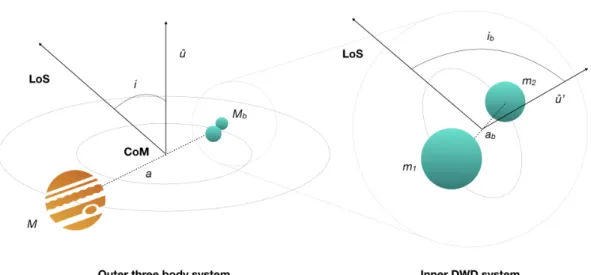
Fig. 1. Geometry of the outer three-body system (DWD+planet/BD) and inner compact two-body system (DWD). The quantities ˆu and ˆu0denote
the directions perpendicular to the outer and inner orbital planes, respectively. The acronyms LoS and CoM stand instead for line of sight and centre of mass (of the whole three-body system).
is implemented in the binary population synthesis either by parametrising the conservation equation for energy (through the α parameter) or that for angular momentum (through the γ parameter) (seeIvanova et al. 2013, for a review). In particular, the γ-prescription was introduced with the aim to reconstruct the evolution path of observed DWDs byNelemans et al.(2000);
Nelemans & Tout(2005). In the model adopted for this study, γα, we allowed both parametrisations; the γ-prescription was applied unless the binary contains a compact object or the CE is trig-gered by a tidal instability. It has also been shown that γα model describes observations better than the model in which only α-prescription is employed (Toonen et al. 2012). Future optical surveys such as the Large Synoptic Survey Telescope (LSST;
LSST Science Collaboration 2009) will provide large samples of new DWDs that will help to further constrain CE evolution for these systems (Korol et al. 2017).
Next, we distributed DWDs in a Milky Way-like galaxy according to a star formation history. We adopted a simpli-fied Galactic potential composed of an exponential stellar disc and a spherical central bulge. Similarly to Ruiter et al.(2009);
Lamberts et al.(2019), we found that the contribution of the stel-lar halo to the total amount of detectable GW sources is at most of a few percent. Thus, it is not included in this study. We pop-ulated the disc according to the star formation rate (SFR) from
Boissier & Prantzos(1999) and assumed the current age of the Galaxy to be 13.5 Gyr. To model the bulge of the Milky Way we doubled the SFR in the inner 3 kpc as inNelemans et al.(2001a). The detailed description of the Galactic model is presented in Korol et al.(2019). Finally, we assigned binary inclination angle ib, drawn from a uniform distribution in cos ib. Thus, each
DWD in the catalogue is characterised by seven parameters: m1, m2, Pb, ib, the Galactic latitude l and longitude b, and the
distance from Sun d (see Fig.1).
To obtain a sub-sample of DWDs detectable by LISA we employed the Mock LISA Data Challenge (MLDC) pipeline, designed for the analysis of a large number of GW sources simultaneously present in the data (e.g. Littenberg et al. 2013;
Cornish & Robson 2017). This is realised throughout an itera-tive process that is based on a median smoothing of the power spectrum of the input population to compute the overall noise level (instrument plus confusion from the input population). The resolved sources (i.e. those with S/N > 7) are extracted from the data until the convergence. We adopted the LISA noise curves
and orbits according to the latest mission design, the nominal mission duration of four years and the extended mission duration of eight years (Amaro-Seoane et al. 2017).
We find approximately 26 × 103 and 40 × 103 detached
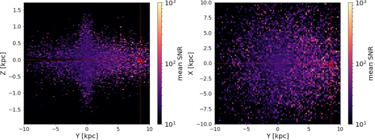
DWDs with S/N > 7 for the nominal four years and extended eight years of the LISA mission duration, respectively. Figure2
illustrates the distribution of detected DWD in our mock Galaxy showing that GW detections can map both disc and bulge at all latitudes. We represent the mean signal-to-noise ratio (S/N) per bin in colour.
We note that in this work we focus on detached DWD binaries only. In principle, other Galactic binaries composed of compact objects (such as WD – neutron star and double neutron stars) and accreting systems could also host a CBP/BD. However, these are significantly less abundant in the Milky Way (e.g. Nelemans et al. 2001a), and thus would not affect much our estimates. In addition, GW signal of accreting systems contains an imprint of the mass-transfer process, which could affect the detection of circumbinary companions. We leave these investigations for future work.
3.2. Exoplanet and brown dwarf injection
Since the WD pollution effect supports evidence of dynamically active planetary systems around single WDs (Sect.2.1) and since no data are available for the binary WD case, we set the WD pol-lution upper limit occurrence rate (i.e. 50%Koester et al. 2014) to be the occurrence rate (O.R.) of the synthetic population of SSOs orbiting DWD. We neglected the presence of an external third star and we assumed that pollution derives from asteroidal or moon material, rather than cometary material. We also rejected exceptions such as the capture of a free-floating planet at thou-sands of astronomical units, and we assumed that each DWD can harbour only one SSO; we briefly discuss the implications of considering multiple circumbinary objects in Sect.5.
For the following we note that co-evolution of the binary plus SSO was neglected, and that the SSO population was injected into already formed WD-WD systems in which the stability cri-terion (P & 4.5 Pb) ofHolman & Wiegert(1999) was always
satisfied.
In accordance with the pollution O.R. employed in this investigation, we set the SSO maximum distance (a) to be the approximate maximum limit for pollution to occur. Given
Fig. 2.Signal-to-noise map of DWDs detected by LISA (4 yr) in the galactocentric Cartesian coordinate system. The colour represents the mean
S/N per bin. The red triangle identifies the position of the LISA detector in our simulation.
that the maximum distance at which those asteroids reside around DWDs is completely unconstrained (Veras et al. 2019), we assumed 200 au to be a reasonable distance at which the SSO could still perturb asteroids which lie outwards or inwards towards the binary.
We set a uniform SSO inclination in cos i (cf. Fig.1) and uniform initial phase φ0between 0 and 2π. Given that the planet
distribution function is unknown and that no compelling physi-cal motivation for a specific model at wide separations exists for these systems, we tested a combination of various semi-major axis a and SSO mass M distributions, commonly presented in the literature, to measure the number of possible detection of both CBPs and BDs. More specifically we defined the semi-major axis distributions as follows: (A) uniform distribution Ua (0.1–
200 au); and (B) log10uniform distribution log Ua(0.1–200 au);
and (C) log-normal distribution f (x) = A eln(x)−µ/2σ2
/(x2πσ), where A is the amplitude, µ the mean of the log-normal, and σthe square root of the variance.Meyer et al.(2018) give more details and specific values of the parameters; and (D) power-law distribution a−0.61(0.1–200 au) (Galicher et al. 2016).
The mass distributions are as follows: (1) uniform distribu-tion UM(1 M⊕–0.08 M ); and (2) a combination of power law,
M−1.31 (Galicher et al. 2016) between 1M
⊕–13MJ and uniform
distribution for 13 MJ< M < 0.08 M .
3.3. LISA detection of a third sub-stellar object
To model the perturbation induced by the SSO on the GW signal emitted by the DWDs, we followed the procedure pre-sented in Tamanini & Danielski (2019). Figure 1 shows the geometry of the three-body system under consideration. The motion of the DWD around the centre of mass of the three-body system modulates the GW frequency through the well-known Doppler effect. The resulting frequency observed by LISA is written as
fobs(t) = 1 +vkc(t)
!
fGW(t), (1)
where vk is the line-of-sight velocity of the DWD with respect
to the common centre of mass, while fGWis the GW frequency
in the reference frame at rest with respect to the DWD centre of
mass. Since the DWDs observed by LISA do not merge before a time much larger than the observational lifetime of the mission, we can effectively model the emitted frequency with a Taylor expansion around a constant value and only keep the first order term
fGW(t) = f0+f1t + O(t2), (2)
where f0is the frequency when LISA starts taking data and f1is
its first derivative evaluated at the same time. The line-of-sight velocity of the DWDs is instead given by
vk=−K cos ϕ(t), (3)
where we defined the parameters K = 2πG
P
!13 M (Mb+M)23
sin i, (4)
and the orbital phase ϕ(t) = 2πt
P + ϕ0, (5)
both derived assuming an SSO circular orbit. In the expressions above P is the SSO orbital period, M is the SSO mass, Mbis the
DWD total mass, ϕ0is the outer orbital initial phase, and i is the
SSO orbital inclination (cf. Fig.1). The phase of the waveform observed by LISA is then given by
Ψobs(t) = 2π
Z
fobs(t0)dt0+ Ψ0, (6)
where Ψ0 is a constant initial phase. The main contribution of
the Doppler frequency modulation Eq. (1) consists in a period-ical shift of the GW frequency towards higher and lower values around f0. This effect is qualitatively depicted in Fig.3in which
the Doppler modulation has been extremely exaggerated with respect to the perturbation induced by a SSO on a DWDs. In the real case the modulation timescale, of the order of roughly years, is much longer than the period of the GW produced by the binary, roughly minutes, implying that the effect would not be visible by eye.
Time
Strain
Fig. 3. Qualitative example of a DWD waveform with (blue) and
without (orange dashed) the presence of a third body. The Doppler modulation is extremely exaggerated for visualisation purposes.
For each DWDs in our mock catalogue we can thus build a waveform depending on 11 parameters: 8 parameters associ-ated with the DWD, namely ln(A), Ψ0,f0,f1, θS, φS, θL, φL, and
3 parameters associated with the SSO orbit, namely K, P, ϕ0. In
this case θS, φS, θL, φLare the two sky localisation angles and the
two angles defining the orbital geometry of the DWDs, respec-tively (directly related to the inclination iband polarisation angle
ψb; see e.g.Cornish & Larson 2003).
To simulate the response of LISA and perform a parame-ter estimation of the GW waveform, we followedTamanini & Danielski (2019) again. The full expressions for the two lin-early independent signals observed by LISA hI,II(t), including
the LISA antenna pattern functions and effects due to its orbital motion, can be found inCutler(1998);Takahashi & Seto(2002);
Cornish & Larson(2003). For the sake of simplicity we are not reporting those expressions in this work. The S/N of each event is computed as the following:
S/N2= 2 Sn( f0) X α=I,II Z Tobs 0 dt hα(t)hα(t), (7)
where Tobsis LISA observational time period and Sn( f0) is the
one-sided spectral density noise of LISA computed at f0.
Param-eter estimation is performed by employing a Fisher information approach, where we define the Fisher matrix as
Γi j = 2 Sn( f0) X α=I,II Z Tobs 0 dt ∂hα(t) ∂λi ∂hα(t) ∂λi . (8)
Marginalised 1σ errors for each waveform parameter are thus estimated from the square root of the diagonal elements of the covariance matrix, the inverse of the Fisher matrix.
4. Results
We focus first on the properties of the detected population of SSOs (Sect.4.1), showing also how the numbers improve for an extended eight-year LISA mission (Sect.4.2). We then discuss the recovered accuracy on the waveform parameters in Sect.4.3. 4.1. LISA detection of SSOs
As inTamanini & Danielski(2019) we assume that a SSO (either a CBP or a BD) is detected if both K and P parameters are mea-sured with a relative accuracy better than 30%. For every injected SSO population, defined by a combination of semi-major axis a
and mass M distributions (see Sect.3.2), we counted the number of SSOs whose GW perturbation can be detected by LISA.
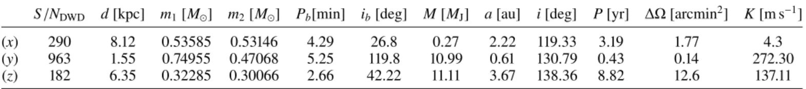
We report in Table 1 the total number and percentage of circumbinary exoplanets and BDs detected during the nominal LISA mission length. For both CBPs and BDs we identified optimistic, pessimistic, and intermediate scenarios. While the first and second represent the cases in which the highest and lowest numbers of CBPs (or BDs) are detected, the last sce-nario represents the case with the median number of detections, rounded by excess. Among the available combinations, the B1 scenario, i.e. that whose injected SSO population follows a log-arithmic a distribution log Ua, and uniform M distribution UM
(see Sect. 3.2), is the optimistic case for both CBPs and BDs with 83 and 2218 detections, respectively. The intermediate sce-nario is represented by C1 (log-normala; UM), and B2 (log Ua;
M−1.31), for CBPs and BDs with 18 and 316 detections,
respec-tively. The pessimistic scenario is represented by A1 (Ua;UM)
and A2 (Ua; M−1.31) with 3 and 14 detections for CBPs and BDs,
respectively. We plot in Fig.4the location in the Milky Way of the detections for the three CBPs scenarios together with a zoom-in on the solar neighbourhood for the optimistic scenario. From Fig.4it is easy to understand that LISA will be able to observe CBPs and BDs orbiting DWDs everywhere in the Galaxy.
Furthermore, for the six scenarios selected above, Figs.A.1
and A.2 (currently appearing after the references) show the distribution of detected CBPs and BDs, respectively, over the CBP/BD separation from the DWD (a), the mass of the CBP/BD (M), the CBP/BD orbital inclination (i), the parameter K, the CBP/BD period (P), the DWD period (Pb), the DWD S/N,
the distance from the Earth (d), the DWD chirp mass (Mc), and
the total DWD magnitude measured in the Gaia G band (GDWD).
To highlight possible observational biases, in Figs.A.1andA.2
we also show the underlying distribution of injected CBPs/BDs in grey.
4.2. Detection rates for an extended LISA mission
We repeated our analysis for an eight-year LISA mission, cor-responding to a possible realistic extension beyond the nominal four-year mission; this can also approximately be considered as ten years of mission operations, the maximal envisaged extended duration, with duty cycle of 80% similar to the LISA Pathfinder (Armano et al. 2016). We used the catalogue of 40 × 103 DWD
detected over the eight years of mission presented in Sect.3.1
injecting SSOs according to the optimistic and pessimistic sce-narios only. The total detections of CBPs and BDs, together with the percentage over the total number of DWDs detected by LISA, are reported in Table2. In the optimistic scenario (B1) we find a total of 215 (4684) detected CBPs (BDs), corresponding to the 0.822% (17.913%) of the total population of detected DWDs, and to an improvement of the 259% (211%) over the detections of the nominal four-year mission. The numbers for the pessimistic scenarios, (A1) for CBPs and (A2) for BDs, are instead 8 (43) detected CBPs (BDs), corresponding to 0.02% (0.107%) of the total DWD population, and to an improvement of the 267% (307%) over the 4 yr detections.
In the hypothesis of eight years of observations, LISA will be able to detect SSOs with longer period P and consequently larger separation a. These are the SSO orbital parameters that present a significant improvement with respect to the four-year case, i.e. for which a larger range of measured values is recov-ered, instead of only a larger number of detections within the same parameter interval. We plot for comparison in Fig.5 the distributions (injected and recovered) of these two quantities
Table 1.Number of planetary detections depending by the different combinations of mass and semi-major axes distributions. DETECTIONS (4 yr)
(A) Ua(0.1–200 au) (B) log Ua(0.1–200 au) (C) log Normala(0.1–200 au) (D) a−0.61(0.1–200 au)
CBPs BDs CBPs BDs CBPs BDs CBPs BDs
(1) UM(1M⊕– 0.08 M ) 3 (0.011%) 79 (0.302%) 83 (0.317%) 2218 (8.482%) 18 (0.069%) 503 (1.924%) 28 (0.107%) 820 (3.136%)
(2) M−1.31 6 (0.023%) 14 (0.054%) 30 (0.115%) 316 (1.209%) 5 (0.019%) 85 (0.325%) 13 (0.050%) 131 (0.501%)
Notes.In bold the minimal and maximal values for both CBPs and BDs. The percentage is computed over a total of 26 148 DWDs (visible during the nominal LISA mission length).
10
0
10
Y [kpc]
10
5
0
5
10
X [kpc]
GC
Scutum-Centaurus Arm
Perseus Arm
(B1)
GW BD
Transit
Microlensing
RV
Imaging
GW CBP
2
0
2
y [kpc]
2
0
2
x [kpc]
ZOOM-IN
(B1)
Transit
Microlensing
RV
Imaging
GW BD
GW CBP
10
0
10
Y [kpc]
10
5
0
5
10
X [kpc]
GC
Scutum-Centaurus Arm
Perseus Arm
(C1)
GW BD
Transit
Microlensing
RV
Imaging
GW CBP
10
0
10
Y [kpc]
10
5
0
5
10
X [kpc]
GC
Scutum-Centaurus Arm
Perseus Arm
(A1)
GW BD
Transit
Microlensing
RV
Imaging
GW CBP
Fig. 4. Optimistic (top left, B1) with its zoom-in on the solar region (top right, heliocentric coordinates), intermediate (bottom left, C1), and
pessimistic (bottom right, A1) scenarios. Each plot shows the location of the binary WD system with a planetary companion (red) and BD (green) detection through GWs. In each panel we also plot the known detected exoplanets’s host-star (see legend for colour scheme; data fromhttps:// exoplanetarchive.ipac.caltech.edu). We note that data overlay a face-on black and white image of the Milky Way for Galactic location
reference purposes.
for both time frames of eight and four years. In general the longer the LISA observational period, the longer the SSO period and separation that will be recovered. This can be easily visu-alised in Fig. 5 where the eight-year bulk of detected CBPs
(BDs), presents periods up to ∼12 (∼30) yr, compared to only ∼6 (∼10) yr over a four-year mission. A similar trend is observed for the separation a, as of course this is directly related to the period.