HAL Id: halshs-00206326
https://halshs.archives-ouvertes.fr/halshs-00206326
Submitted on 17 Jan 2008
HAL is a multi-disciplinary open access archive for the deposit and dissemination of sci-entific research documents, whether they are pub-lished or not. The documents may come from teaching and research institutions in France or abroad, or from public or private research centers.
L’archive ouverte pluridisciplinaire HAL, est destinée au dépôt et à la diffusion de documents scientifiques de niveau recherche, publiés ou non, émanant des établissements d’enseignement et de recherche français ou étrangers, des laboratoires publics ou privés.
A note on the consequences of an endogenous
discounting depending on the environmental quality
Alain Ayong Le Kama, Katheline Schubert
To cite this version:
Alain Ayong Le Kama, Katheline Schubert. A note on the consequences of an endogenous discounting depending on the environmental quality. Macroeconomic Dynamics, Cambridge University Press (CUP), 2007, 11 (2), pp.272-289. �10.1017/S1365100507060063�. �halshs-00206326�
A note on the consequences of an endogenous discounting
depending on the environmental quality
A. Ayong le Kama
Université de Lille 1 and Commissariat général du Plan E-mail: [email protected]
K. Schubert
EUREQua, Université de Paris 1 E-mail: [email protected]
November 9, 2005 –revised version
Abstract
Our intention is to study, in the framework of a very simple optimal growth model, the consequences on the optimal paths followed by consumption and the environmental quality of an endogenous discounting. Consumption directly comes from the use of environmental services and so is a direct cause of environmental degradation. The environment is valued both as a source of consumption and as an amenity. For a sustainability concern, we intro-duce an endogenous discount rate growing with the environmental quality, and compare the optimal growth paths with the ones obtained in the usual case of exogenous and constant discounting. We show that the convergence of the environmental quality towards a steady state occurs only for a very special con…guration of the parameters in the exogenous dis-counting case, while it occurs generically in the endogenous disdis-counting one. This happens for a utility discount rate becoming su¢ ciently high when the environmental quality is high and su¢ ciently low when the environmental quality is poor. In this case then, endogenous discounting with a positive marginal discount rate allows us to avoid the depletion of the environment.
Keywords: Endogenous discounting, Sustainability, Environment JEL codes: O41, Q0, E6
Corresponding author. Address: EUREQua, U.M.R. n 8594 CNRS, Université de Paris I, Maison des Sciences Économiques, 106–112 bd. de l’Hôpital, 75647 Paris Cedex 13, France.
1
Introduction
Optimal growth models usually make the assumption of a constant and strictly positive utility social discount rate. This practice has long been questioned, but is still widely used, maybe because of the lack of a convincing alternative (Heal (2001)).
The …rst doubt goes back at least to the well known criticisms by Ramsey and Harrod of a strictly positive utility social discount rate (Ramsey (1928), Harrod (1948)), and has led to the so-called undiscounted utilitarianism. But Koopmans (1960) has stressed the drawbacks of this approach: it usually leads to unrealistically high optimal saving rates for the present and near-future generations, and so to a sacri…ce of the present and of the near future instead of the supposed sacri…ce of the far future implied by a positive discount rate. Nevertheless, the temptation of a zero rate of discount is still very present as far as the environment is concerned because of the very long horizon often involved in environmental matters1 (see, for a
comprehensive view of discounting and the environment, the contributions collected in the book edited by Portney and Weyant (1999)).
The usual approach has been challenged by authors arguing that the utility discount rate should be neither constant and positive nor zero, but should be decreasing in the course of time. They claim that empirical evidence supports that decrease. Harvey (1994), Heal (1998), Loewenstein and Prelec (1992), Laibson, (1996), (1997) or Barro (1999) propose formulas of decreasing discounting justi…ed by considerations of individual psychology. But the choice of a utility discount rate in normative models is an ethical one, as stressed by Heal (1998), (2001) or Ayong Le Kama (2001), and it is less than obvious that a social planner should only re‡ect in this choice the representative consumer’s psychology. Gollier (2002a), (2002b) and Weitzman (1998) justify decreasing discounting in a partial equilibrium set-up by the uncertainty on the future growth rate of the economy or on the future interest rate. Li and Löfgren (2000) study an economy with heterogeneous agents di¤ering by their utility discount rate (constant and exogenous) but identical in all other respects. They show that this economy behaves as if there was a unique representative agent with a decreasing discount rate, tending in the long run towards the rate of the more patient agent. Here the decreasing discount rate is not an assumption but a consequence of the heterogeneity.
Another strand of literature, disconnected from environmental concerns, studies the question of habit formation, and introduces a utility discount factor depending on present and past consumption levels (Epstein (1987), Becker, Boyd and Sung (1989), Obstfeld (1990), Das (2003)). Obstfeld (1990) gives a formal treatment of the simple optimal growth model with this utility discount factor, and concludes that most of the time this assumption does not qualitatively change the optimal growth paths, in comparison with the case of an exogenous constant discount rate.
We want here to extend Obstfeld’s approach to a growth model in which environment matters (Pittel (2002) has the same objective in a di¤erent framework). We consider two ways by which the environmental quality could a¤ect the social intertemporal welfare: the usual direct e¤ect of the current level of environmental quality on instantaneous utility (amenity e¤ect), and a less usual indirect e¤ect of current and past levels of environmental quality on the utility discount factor. This discount factor now depends on the path of environmental quality through time. Utility is no longer time-separable, tastes are intertemporally dependent. The discount rate depends on the current state of the environment. Besides, we make the assumption of a positive marginal impatience: the discount rate increases with the level of the environmental quality.
It is possible to rationalize this ethical choice of an endogenous utility discount rate depending on the environmental quality and increasing with it by a sustainable development motive. Society could express in this way a form of intergenerational altruism, consisting in deciding to discount
1
the future at a rate all the lower since the environmental quality is low. That could be a way of introducing sustainability concerns in optimal growth models2.
We then try to elucidate the consequences of such an ethical choice. These consequences are very hard to assess in complex growth models with capital accumulation. We thus use here a simple framework where consumption directly comes from the use of environmental services, and so directly causes environmental degradation3.
We …rst study the evolution of the economy and the environment with an exogenous and con-stant discount rate (section 2), as a benchmark for the study of the endogenous utility discount case. We present and discuss in section 3 the assumptions made about the endogenous discount factor and their consequences, and then characterize all the types of optimal paths that the economy can follow under these assumptions. We show that the convergence of the environmen-tal quality towards a steady state occurs only for a very special con…guration of the parameters in the exogenous discounting case, while it occurs generically in the endogenous discounting one. This happens for a utility discount rate becoming su¢ ciently high when the environmental quality is high and su¢ ciently low when the environmental quality is poor. Section 4 concludes.
2
The economy with a constant discount rate
2.1 The model
We introduce an optimal growth model with an environmental asset. This asset can be seen as natural capital or as the environmental quality. It is valued both as a source of consumption of environmental services and as a stock of amenities. The stock of environmental asset S is depleted by consumption C, but regenerates itself at a rate m > 0 taken as constant for simpli…cation. Its dynamics is then described by
:
St= mSt Ct: (1)
The objective of the social planner is to maximize the present value of the life-time utility of the representative consumer over an in…nite horizon. The representative consumer derives felicity4 u(:) not only from consumption, but also from environmental quality. The future felicities are discounted at the constant rate > 0. Let C = [Ct]10 and S = [St]10 represent
some consumption and environmental quality paths respectively. The social planner seeks to maximize max U (C; S) = Z +1 0 e tu (Ct; St) dt; (2) subject to 8 < : _ St= mSt Ct; Ct 0; St 0; S0 given. (3) 2
It could be interesting to study the market economy, where private agents, unaware of sustainability concerns and/or considering the environmental quality as an externaliy, would discount exponentially, and to look at the way the optimal solutions with endogenous discounting could be implemented.
3
It is in some sense the worst possible case: there exist neither technical progress enhancing the transformation of environmental services into consumption, nor substitution possibilities between environmental services and man-made capital. There is no means of improving the environmental quality except by natural regeneration. In such a framework, consumption and environmental quality necessarily evolve together in the long run: both increase, or both decrease, or both converge towards a stationary state.
4We follow the convention of Arrow and Kurz (1970) in referring to the subutility functions as felicities. In
Assumption 1. The felicity function u (:) is continuous, twice di¤ erentiable, and possesses the following properties5: 8C; S > 0; uC > 0; uS > 0; uCC 0: It is also concave with respect
to its two arguments: uCCuSS (uCS)2 0:
The constant-value Hamiltonian of the previous problem is H = u (C; S) e t+ e [mS C] ;
where e 0 is the co-state variable associated with the environmental quality. The …rst order necessary conditions then give us
= uC; (4a)
:
= m (C; S)C
S; (4b)
where = ee t, and the transversality condition writes lim
t!1e t
tSt= 0: (3c)
(C; S) SuS
CuC > 0 by assumption 1 is the ratio of the values of environmental quality and
consumption, both evaluated at their marginal felicity. (:) then re‡ects the “relative preference for the environment” of the representative agent.
Di¤erentiation of equation (4a) with respect to time leads to the following result:
: = 1 : C C + 2 : S
S; where 1 = CuCC/ uC < 0 is the elasticity of the marginal felicity of consumption
with respect to the level of consumption and 2 = SuCS/ uC S 0 is the elasticity of the marginal
felicity with respect to the level of environmental quality. Substituting this relationship into (4b) yields 1 : C C + 2 : S S = m (C; S) C S: (5)
2.2 The balanced growth path (BGP)
2.2.1 Existence of a BGP
Given the equation of motion of the environmental quality (1), if the growth rate of the en-vironmental quality is constant along the optimal path then the ratio C=S is also constant, which indicates that C and S grow at the same rate. Let g be this common rate. We have C=S = m g: Substituting g into (5) leads to
g = (1 + (C; S))m
1+ 2 (C; S)
:
Therefore, the feasibility of the BGP, that is the constancy of g; requires:
Assumption 2. (i) The elasticities of the marginal felicity of consumption with respect to con-sumption, 1; and environmental quality, 2; are constant; (ii) the relative preference for the environment is constant, i.e. (C; S) = ; 8 (C; S)6.
5
uC and uS are the …rst partial derivatives of the function u (:) with respect to its arguments C and S: uCC
is likewise the second partial derivative, using obvious notation.
6
Smulders and Gradus (1996) show that (ii) is a necessary condition for the existence of a balanced growth path when the stock of environmental resource is a source of felicity.
These restrictions7 give rise to a non-separable felicity function of the CRRA-type:
u (C; S) = CS
1 1=
1 1= ; (6)
where = 1= 1 > 0 is the intertemporal elasticity of substitution of consumption. Assumption 3. < 1:
This assumption is su¢ cient to ensure the concavity of the felicity function8. It implies that
the marginal felicity of consumption decreases with the level of environmental quality: uCS< 0:
Furthermore, with < 1 the felicity function (6) is negative and thus bounded from above. It is easy to show that, with the speci…cation of the felicity function (6), the growth rate along the BGP is
g = m
1 + ; (7)
which may be positive or negative, depending on the parameters9. We can also notice that
the optimal growth rate is bounded from above: g m = lim !0g: m therefore re‡ects the highest growth rate that society can expect; it depends on the regenerative capacities of the environment.
Besides, as S is evolving along the BGP at the rate g and at the rate m (m g); the transversality condition (3c) is ful…lled if and only if (g m)(1 + ) < 0 i.e. g < m: Given that we have assumed < 1, the upper bound of g is strictly lower than m: g m < m: The transversality condition is always satis…ed.
2.2.2 Properties of the BGP
Introducing the stationary variable x = CS; we easily show, using the equation of motion of the environmental quality (1) and equation (5), that the dynamic system characterizing the evolution of the economy and the environment reduces to a single equation in x;
_x
x = (1 + )(x ex); (8)
whereex > 0 is the stationary ratio of consumption to environmental quality along the BGP. By (1) and (7), we have:
e
x = m g = (1 )m +
1 + : (9)
Equation (8) is unstable. If the x ratio is higher than ex; the environmental quality will be consumed completely, and if on the contrary it is lower, the environmental quality will grow without bounds and consumption will be driven to zero. The x ratio then takes from the initial time its stationary valuex; and initial consumption is Ce 0 =xSe 0 = (1 )m +1+ S0:
7
Despite the lack of generality that these restrictions imply, they allow us to study the e¤ect of endogenous discounting in a framework where the benchmark – the case with constant and exogenous discounting – consists in a balanced growth path.
8
We see easily that the necessary and su¢ cient condition for concavity is 1+ : < 1is then su¢ cient, and we restrict ourselves to this case for technical reasons (see below).
9
The growth rate of consumption and environmental quality along the BGP will be positive if the natural regeneration and the preference for the environment are su¢ ciently high, and if the discount rate is low enough.
3
The economy with an endogenous discount rate
3.1 The model
We now introduce an economy where the social planner uses a discount factor based on the historical path of the environmental quality. In all other respects, the economy is the same as in the previous section. The intertemporal discounted utility function, with variable discount rate, of a representative consumer is now given by
U (C; S) = Z +1
0
e tu (C
t; St) dt; (10)
where the felicity function u (:) satis…es assumptions 1, 2 and 3. The future felicities are dis-counted at time t with a discount factor equal to e t; where
t 0 is assumed to depend on
the past and current levels of the environmental quality, as described by the following equation:
t= Z t 0 (S )d : (11) (St) = d ln(e t)
dt 0; 8St; is the utility discount rate at time t10.
In the case of an endogenous discounting depending on the past and current levels of con-sumption, there is considerable disagreement over whether the marginal discount rate should be positive or negative (see Obstfeld (1990)). Loosely speaking, a positive marginal rate means that rich people are more impatient than poor ones. This assumption is frequently made in the literature related to the question of habit formation, but never satisfactorily justi…ed (see Epstein (1987)). Obstfeld (1990) justi…es his adoption of this assumption by the fact that it is necessary for the convergence of his model. Das (2003) shows that this is not a general property of models with habit formation, which can, under some additional assumptions, be stable even with a negative marginal discount rate. Whatever the psychological explanations that underline each approach, our view is that the …nal choice is normative. Moreover, we think that the fact that impatience should be increasing or decreasing with the consumption of private goods doesn’t imply anything about how impatience should evolve with the public natural capital11. We require:
Assumption 4. 0(S) > 0 and 00(S) < 0; 8S > 0:
Our choice of a discount rate increasing with the environmental quality is justi…ed by the outcomes of the current debate about discounting and the environment (see Portney and Weyant (1999) for a comprehensive view of this debate). The main point is to …nd how to properly take into account the welfare of the far future generations, that the traditional exogenous exponen-tial discounting makes quite irrelevant, without sacri…cing the welfare of the present ones; or, as has been stressed by Chichilnisky (1996), how to avoid any dictatorship of the present and of the future. One possible way is to use hyperbolic (decreasing) discounting, but it leads to time inconsistent choices. Our approach allows us to avoid this. In this context, the positive marginal
1 0The preference structure, as speci…ed in (10), is recursive in the sense that is allowed to depend on the
past and current levels of the environmental quality, as described by equation (11). Thus, a change in the present level of environmental quality will not only have an e¤ect on the current level of felicity, but also on the entire future felicity stream.
1 1
This is the reason why our model does not reduce to the familiar AK framework of the endogenous growth theory, even if it seems formally identical: the AK model deals with man-made capital, which is a private good, while we want to study endogenous discounting depending on the natural capital, which is a public or at least a merit good.
discount rate re‡ects the sustainability motive that here underlies endogenous discounting: con-cerned by intergenerational equity, the society chooses to discount at a rate all the smaller since the environmental quality is low, because in this case environmental questions become pressing. The idea is that an endogenous discounting with a positive marginal discount rate depending on the level of the environmental quality should help to prevent or to limit further deteriorations of the environment.
Following Obstfeld (1990), we consider tas a second state variable that accounts for
accu-mulated impatience12: Di¤erentiating (11) with respect to time yields
_t= (St): (12)
The social planner’s program is therefore to maximize (10) subjects to (1) and (12) together with the initial conditions (S0 and 0 given) and non-negativity constraints (Ct 0; St 0).
The constant-value Hamiltonian of the social planner’s problem is
H C; S; ; e; e = u (C; S) e + e [mS C] e (S); (13)
where e 0 is the co-state variable associated with environmental quality, and e is the co-state variable associated with the “stock of accumulated impatience” (Obstfeld (1990)).
Applying Pontryagin’s maximum principle, we get the following …rst-order necessary condi-tions for optimality:
uC = ; (14a) : = (S) m C S + 0(S); (14b) : = (S) u(C; S); (14c)
where = ee and =ee (thus _ (S) =
:
ee ), together with the transversality condition13
lim
t!1H (t) = 0: (15)
Note that, as Obstfeld (1990) points out, when converges to a de…nite long term value, as will be the case below, the third equation (14c) of this system can be integrated into
t= Z 1 t u(Cs; Ss)e Rs t (S )d ds = e t Z 1 t e su(C s; Ss)ds; (16)
which means that t corresponds to the discounted present value of the future ‡ow of felicities from the standpoint of time t. Given that we have assumed a negative felicity function, we also
have t 0:
We prove in the Appendix that assumptions 3 and 4 ensure the strict concavity of the maximized Hamiltonian H S; ; e;e = maxCH C; S; ; e; e with respect to S and . So
the necessary conditions are also su¢ cient for an optimum (Seierstad and Sydsaeter (1987)). We now reduce the system (14a)-(14c) into a more tractable one. Following Palivos, Wang and Zhang (1997), recall that, along the optimal path, dH/ dt = @H/ @t: Since the social plan-ner’s program considered here is autonomous, @H/ @t = 0; thus the Hamiltonian is independent
1 2
Due to the non constant discount rate, Pontryagin’s maximum principle cannot be applied directly. We need this state variable to solve the problem within the standard optimal control approach.
1 3
of time along the optimal path. This and the transversality condition (15) imply that H (t) = 0 8t along the optimal path. We can therefore deduce
= 1
(S)[u (C; S) + (mS C)] : (17)
The system (14a)-(14b) then writes
= uC; (18a) _ = (S) m C S + 0(S) (S) u (C; S) (C mS)uC uC : (18b)
3.2 The optimal paths
Given assumptions 1 and 2, the di¤erentiation of the …rst-order condition (18a) with respect to time yields _ = 1 : C C + (1 1 )S_ S:
Substituting the dynamics of the environmental quality (1) and the …rst-order condition (18b) into this equation, we show that the dynamics of consumption along the optimal path is
: C C = C S (S) + ( (1 )) m + "(S) 1 1 C S m ; (19)
where "(S) = S(S)0(S) is the elasticity of the utility discount rate (:) with respect to the environ-mental quality. "(S) is positive under assumption 4. If we reintroduce the variable x = C=S; the dynamic system characterizing the evolution of this economy is given by the motion of the ratio of consumption to environmental quality along the optimal path:
:
x
x = 1 + +1 "(S) [x (1 )m] (S); (20)
together with the one of the environmental quality (1). Let us assume that the utility discount rate is bounded:
Assumption 5. (i) limS!1 (S) = is …nite, and (ii) limS!0 (S) = 0:
The …rst part of this assumption seems reasonable: it means that when the environmental quality becomes very high the discount rate remains bounded. can be interpreted as the utility discount rate that the social planner would choose if economic activity did not harm environmental quality, which could remain always high. The second part of this assumption just introduces the notation used for the lower bound of the utility discount rate, eventually equal to zero14.
Now we can study all the types of optimal scenarios that can occur with endogenous dis-counting, given the parameters of the economy.
1 4
An example of discount rate statisfying assumptions 4 and 5, with = 0;is: (S) = 1 e S ; > 0:
3.2.1 The stationary state
Let us …rst look at the existence of a stationary state of the dynamic system (1) and (20). A stationary solution (x ; S ) of this dynamic system is characterized by x =:
:
S = 0: Thus, equation (1) implies x = m: Substituting this into (20), we easily see that stationary solutions are values S satisfying the following equation:
(S) = m 1 + +
1 "(S) : (21)
Assumption 6. "0(S) 0; 8S:
This assumption demands that the elasticity of the utility discount rate is decreasing in S. It seems reasonable, and besides it is necessary to ensure the stability of the stationary solution (see below).
Proposition 1 : Under assumptions 1-6, there exists a unique stationary equilibrium (x ; S )
characterized by ( x = m; (S ) = m h 1 + +1 "(S ) i ; (22)
if and only if m(1 + ) and mh1 + +1 "(0)i i.e. if and only if the upper bound of the utility discount rate is high enough vis-à-vis the relative preference for the environment and the natural regeneration rate and the lower bound low enough15:
Proof. Let us consider the function f (S) = mh1 + +1 "(S)i> 0 which corresponds to the RHS of (21). A solution S of (21) will be such that (S ) = f (S ) : We know, by assumptions 4 and 5, that (S) is strictly increasing from its lower bound (eventually equal to zero) to its upper bound : Besides, f (S) is positive, and we have f0(S) = m1 "0(S) 0 under assumption
6 above. Palivos et al. (1997) show (Lemma 1 p. 212) that under assumption 5 (i) we have limS!1S 0(S) = 0; i.e. limS!1"(S) = 0: Then f (S) decreases monotically for S = 0 to +1 from f (0) = mh1 + +1 "(0)i to m(1 + ). There exists therefore a unique value S such that (S ) = f (S ) if and only if ; \ [m(1 + ); f(0)] 6= ?; which reduces to m(1 + ) and f (0):
Proposition 2 : Under assumptions 1-6, the unique stationary equilibrium (x ; S ) is a saddle-point.
Proof. We can show that the Jacobian matrix of the dynamic system (1) and (20) is
J = 0 S
m 1 m"0(S ) 0(S ) (S )
! :
We then have trJ = (S ) > 0 and
det J = mS
1 m"
0(S ) 0(S ) < 0
because "0(S ) 0 by assumption 6 and 0(S ) > 0 by assumption 4.
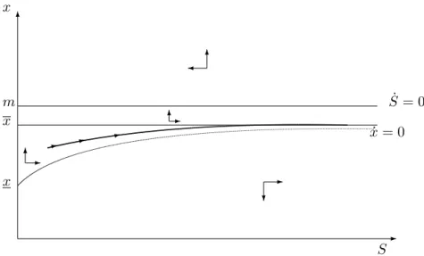
Propositions 1 and 2 state that endogenous discounting associated with a high upper bound of the utility discount rate and a small lower bound of this rate leads to the convergence of the economy towards a locally stable stationary state. In the exogenous discounting case there is a unique con…guration of the parameters ensuring g = 0: the discount rate must satisfy = (1+ )m; whereas the existence of a stationary state is generic in the endogenous discounting case. Besides, the steady state is unstable in the exogenous case, whereas it is saddle-path stable in the endogenous one. This result means that endogenous discounting with a utility discount rate becoming su¢ ciently high when the environmental quality is high and su¢ ciently low when the environment is very depleted allows society to stabilize the environmental quality, which would either collapse or grow in…nitely with exogenous discounting. See …gure 1, where the
_x = 0 curve is growing, and admits x = (1 )m + 1+ as an asymptote16.
-6 6 ? -? -6 * 1 9 9 S x m x S _ S = 0 _x = 0 x
Figure 1: The convergence towards a stationary state. Case > m(1 + ) i.e. x > m and f (0) i.e. x m
More technically, this result shows that the endogenous discounting allows a stabilization of the environmental quality when the bounds of the discount function are such that the range of feasible values of the ratio of consumption to environmental quality includes the regenerative capacity of the environment, m: That is: for (S) 2 ; ; S 2 [0; +1[ ; a necessary condition for the existence of a stationary solution is m 2 [x; x[ :
Let us now characterize the optimal paths when no stationary solution exists.
3.2.2 The asymptotically balanced growth path
Adapting Palivos et al. (1997), we say that a solution of the system (1) and (20) is an asymp-totically balanced growth path if limt!1SS_ exists and is …nite (the path is nondegenerate if this limit is strictly positive) and if limt!1xx_ = 0. Palivos et al. (1997) show that necessary condi-tions for the existence of an asymptotically balanced growth solution of this type of problem is an asymptotically constant discount rate and an asymptotically constant elasticity of marginal felicity. These two conditions are by assumption ful…lled here. We then obtain the following. Proposition 3 : Under assumptions 1-6, there exists a unique nondegenerate asymptotically
1 6
We show easily that the locus _x = 0is a curve x(S) increasing in S from x(0) = x = (1 )m+1+ +
1 "(0) to
limS!1x(S) = (1 )m+1+ +1 limS!1"(S):It will be shown below that limS!1"(S) = 0:So limS!1x(S) =
balanced growth path characterized by 8 < : g = m 1+ ; x = (1 )m + 1+ ; (23)
if and only if < m(1+ ) i.e. the upper bound of the utility discount rate is low enough vis-à-vis the relative preference for the environment and the natural regeneration rate. If = m(1 + ); we have a degenerate asymptotically balanced growth path with g = 0:
Proof. Let us suppose that there exists a constant and strictly positive growth rate g such that limt!1SS_ = limt!1CC_ = g: We then have limt!1xx_ = 0: Because g > 0, we have limt!1S = +1 and assumption 5 (i) can be used. As shown by Palivos et al. (1997) (Lemma 1 p. 212), we then have limS!1"(S) = 0: The long term of the system (1) and (20) is then given by
g = m x;
0 = (1 + )(x (1 )m) ;
from which we deduce (23). By construction, this solution is valid if and only if g > 0; i.e. < m(1 + ). The case = m(1 + ) is straightforward.
We may notice that the asymptotic growth rate g is exactly the same as the balanced growth rate g of the problem with exogenous discounting, provided that = (see equation (7)). Then if the upper bound of the utility discount rate is exactly the rate that would be chosen by the social planner in the case of exogenous discounting, the endogenous discounting economy follows in the long run the same path as the exogenous one, provided that this rate is low enough.
The system (1) and (20) is a dynamic system involving two variables: the environmental quality S; which grows asymptotically at a constant rate, and the ratio of consumption to environmental quality x which is stationary in the long run. Moreover, equation (20) makes the growth rate of x depend on the level of S; and so S cannot be easily eliminated to obtain a system involving two variables stationary in the long run. Nevertheless, we obtain the following results.
Proposition 4 : Under assumption 1-6, if the upper bound of the utility discount rate is low enough (i.e. if m(1 + )), then along the asymptotically balanced growth path:
(i) x is lower than its long run value, i.e. xt< x 8t;
(ii) the growth rate of the environmental quality is higher than its long run value, i.e. _St=St> g
8t:
Proof. It is easy to show that equation (20) can be rewritten as:
:
x
x = 1 + +1 "(S) (x x) + (S) +
2 "(S)
(1 ) (1 + ):
This equation shows that for any given value of x such that x x; _x=x > 0 and x diverges, which is impossible. We therefore deduce that x < x 8t (this shows the …rst part of the proposition). We then have _S=S = m x = g + x x > g.
Propositions 3 and 4 indicate that endogenous discounting associated with an upper bound of the utility discount rate relatively low leads to an asymptotically balanced growth path, and that in the short run the environmental quality grows faster than in the long run at the expense of lower consumption. Society is less impatient to consume in the short run than in the long
-6 6 6 -6 -? : : : S x m x _ S = 0 _x = 0 x
Figure 2: The asymptotically balanced growth path. Case m(1 + ) i.e. x m
3.2.3 The asymptotical depletion of the environmental quality
We now consider the last feasible case. This case involves a high lower bound of the utility discount rate, such that > f (0):
Proposition 5 : Under assumptions 1–6, if > m 1 + +1 "(0) (i.e. if the lower bound of the utility discount rate is high enough vis-à-vis the preference for the environment and the natural regeneration rate), an asymptotical depletion of the environmental quality occurs, with
8 < : g = m 1+ + 1 "(0) < 0; x = (1 )m +1+ + 1 "(0): (24)
Proof. When the environmental quality decreases towards 0, the long term of the system (1) and (20) is given by
g = m x;
0 = (1 + +1 "(0))(x (1 )m) ;
from which we deduce (24). By construction, this solution is valid if and only if g < 0; i.e. > m 1 + + 1 "(0) = f (0).
Proposition 6 : Under assumptions 1–6, if > m 1 + +1 "(0) , then along the path of asymptotical depletion of the environmental quality:
(i) x is higher than its long run value, i.e. xt> x 8t;
(ii) the environmental quality decreases more quickly than in the long run, i.e. _St=St< g 8t:
Proof. It is easy to show that equation (20) can be rewritten as
: x x = 1 + +1 "(S) (x x) + ( (S)) + 2 ("(S) "(0)) (1 ) 1 + +1 "(0) :
This equation shows that if x x; _x=x < 0 and x converges towards zero, which is impossible given the properties of the felicity function. We therefore deduce that x > x; 8t (this shows the …rst part of the proposition). We then have _S=S = m x = g + x x < g.
Propositions 5 and 6 indicate that when the discount rate is bounded from below at a high value, the optimal solution is an asymptotical depletion of the environmental quality, because the society’s impatience remains high whatever the level of the natural capital. Furthermore, impatience is higher in the short run than in the long run, because the environmental quality is higher and impatience increases with it. This implies that in the short run environmental quality decreases faster, which allows the society to consume more. See …gure 3. In this case, the ratio of consumption to environmental quality is always higher than the regenerative capacity of the environment m: -6 6 ? ? ? -9 9 S x m x _ S = 0 _x = 0 x
Figure 3: The asymptotical depletion of the environmental quality. Case > f (0) i.e. x > m
4
Concluding remarks
This paper has introduced an endogenous utility discount rate depending on the state of the environmental quality. Even if there is a disagreement over whether the marginal discount rate should be positive or negative, in the context of the habit formation literature where the discount rate depends on consumption for a private motive, we make here the assumption of a positive marginal discount rate depending on the state of the environment to re‡ect the social motive of sustainability. In the context of the long-lasting debate about discounting and the environment, this expresses the fact that if the society is concerned by intergenerational equity, it will choose to discount at a rate all the smaller since the environmental quality is low.
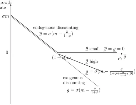
We show within this framework that under both exogenous and endogenous discounting three qualitatively di¤erent scenarios can occur: growth of consumption and the environmental quality to in…nity, decrease to zero, and convergence towards a positive steady state (see …gure 4). This last scenario occurs with endogenous discounting when the discount rate is allowed to vary between bounds and ; with large enough and small enough, while in the exogenous case it occurs only for a discount rate exactly equal to (1 + )m; a razor-edge case. So a stabilization of the environmental quality is more likely to occur with endogenous discounting.
This methodology can be used in applied cost-bene…t analysis. While implying a utility discount rate decreasing in the course of time if environmental conditions worsen, it avoids the problem of time inconsistency and gives a new justi…cation to this decrease.
-6 c c c c c c c c c c c c c c c c c c c c c c c c c c c c c c ca aaa aaa aaaa 0 , growth rate m (1 + )m endogenous discounting g = (m 1+ ) exogenous discounting g = (m 1+ ) g = (m 1+ + 1 (0) ) small g = g = 0 high
Figure 4: The growth rate as a function of (exogenous discounting) and (endogenous dis-counting)
References
Arrow, K., and M. Kurz (1970): Public Investment, the Rate of Return and Optimal Fiscal Policy. Johns Hopkins Press.
Ayong Le Kama, A. (2001): “Sustainable Growth, Renewable Resources and Pollution,” Journal of Economic Dynamics and Control, 25(12), 1911–1918.
Barro, R. (1999): “Ramsey Meets Laibson in the Neoclassical Growth Model,” Quarterly Journal of Economics, 114, 1125–1152.
Becker, R., J. Boyd, and B. Sung (1989): “Recursive Utility and Optimal Capital Accu-mulation. I. Existence,” Journal of Economic Theory, 47, 76–100.
Chichilnisky, G. (1996): “An Axiomatic Approach to Sustainable Development,” Social Choice and Welfare, 13, 231–257.
Das, M. (2003): “Optimal Growth with Decreasing Marginal Impatience,”Journal of Economic Dynamics and Control, 27, 1881–1898.
Epstein, L. (1987): “A Simple Dynamic General Equilibrium Model,” Journal of Economic Theory, 41, 68–95.
Gollier, C. (2002a): “Time Horizon and the Discount Rate,” Journal of Economic Theory, 107, 463–473.
(2002b): “Discounting an Uncertain Future,” Journal of Public Economics, 85, 149– 166.
Harrod, R. (1948): Towards a Dynamic Economy. Macmillan Press, London.
Harvey, C. (1994): “The Reasonableness of Non-Constant Discounting,” Journal of Public Economics, 53, 31–51.
Heal, G. (1998): Valuing the Future: Economic Theory and Sustainability. Columbia University Press.
(2001): “Intertemporal Welfare Economics and the Environment,” mimeo, University of Columbia.
Koopmans, T. (1960): “Stationary Ordinal Utility and Impatience,” Econometrica, 28, 287– 309.
Laibson, D. (1996): “Hyperbolic Discount Functions, Undersaving, and Savings Policy,”NBER Working Paper, 5635.
(1997): “Golden Eggs and Hyperbolic Discounting,” Quarterly Journal of Economics, 112, 443–477.
Li, C.-Z., and K.-G. Lofgren (2000): “Renewable Resources and Economic Sustainability: A Dynamic Analysis with Heterogeneous Time Preferences,” Journal of Environmental Economics and Management, 40, 236–249.
Loewenstein, G., and D. Prelec (1992): “Anomalies in Intertemporal Choice: Evidence and an Interpretation,” Quarterly Journal of Economics, 107, 573–598.
Michel, P. (1982): “On the Transversality Conditions in In…nite Horizon Problems,” Econo-metrica, 50(4), 975–985.
Obstfeld, M. (1990): “Intertemporal Dependence, Impatience, and Dynamics,” Journal of Monetary Economics, 26, 45–75.
Palivos, T., P. Wang, and J. Zhang (1997): “On the Existence of Balanced Growth Equi-librium,” International Economic Review, 38(1), 205–223.
Pittel, K. (2002): Sustainability and Endogenous Growth. Edward Elgar, Cheltenham, UK. Portney, P. R., and J. P. Weyant (1999): Discounting and Intergenerational Equity.
Re-sources for the Future.
Ramsey, F. P. (1928): “A Mathemathical Theory of Saving,”Economic Journal, 138, 543–59. Seierstad, A., and K. Sydsaeter (1987): Optimal Control Theory with Economic
Applica-tions. North Holland, Amsterdam.
Smulders, S., and R. Gradus (1996): “Pollution Abatement and Long-term Growth,” Eu-ropean Journal of Political Economy, 12, 505–532.
Weitzman, M. (1998): “Why the Far Distant Future should be discounted at its Lowest Possible Rate,” Journal of Environmental Economics and Management, 36, 201–208.
Appendix: proof of the strict concavity of the maximized
Hamil-tonian with respect to
S and
The constant value Hamiltonian is given by equation (13) and the …rst order condition for optimality with respect to C is given by equation (14a) and writes uC = e e: With our
speci…-cation of the felicity function (6), this equation gives us the following expression for the optimal consumption: C S; ; e = e S ( 1 1) e ! : We have H S; ; e;e = maxCH C; S; ; e; e = H C ; S; ; e; e : H S; ; e;e = u (C ; S) e + e [mS C ] e (S) = emS e (S) 1 e S 1 :
So HS = em e 0(S) + e S ( 1) 1 e 1 H = 1 e S e 1 ; and HSS = e 00(S) + ( ( 1) 1) e S ( 1) 2 e 1 H = 2 1 e S e 1 HS = e S ( 1) 1 e 1 ;
from which we easily deduce:
HSSH (HS ) 2 = 2 1 e 2 S2 ( 1) 2 e2( 1) + 2 1 e S ( 1) e 1 e 00(S):
Given that by equation (16) we havee = e 0; assumptions 3 and 4 ensure that HSSH (HS )
2