HAL Id: hal-01852010
https://hal.archives-ouvertes.fr/hal-01852010
Operating principle of an active lift turbine with
controlled displacement
Pierre Lecanu, Joel Breard, Dominique Mouazé
To cite this version:
Pierre Lecanu, Joel Breard, Dominique Mouazé. Operating principle of an active lift turbine with
controlled displacement. 2018. �hal-01852010�
Operating principle of an active lift
turbine with controlled displacement
Pierre Lecanu, AJC Innov 401263611
∗7, chemin du Mont Desert 14400 Esquay sur Seulles - France
Joel Breard, LOMC UMR CNRS 6294, Universite du Havre
Dominique Mouaze, M2C UMR CNRS 6143, Universite de Caen
Abstract
The purpose of this article is to present in a simple principle of the turbine ’active lift turbine’ and to realize a calculation approximation of the couple produces by this turbine. For a calculation more elaborate, it is necessary to read the preprint.[6]
1
List of symbols
O : turbine center. A : central gear center. B : satellite gear center.
C : pivot connection between rod and crank. D : pivot connection between rod and slide. E : fixation point of the blade.
Ex : central gear eccentricity (OA = −Ex). Rb : radius of the crank (BC = Rb).
Rg : radius of the central gear or satellite gear (AB = 2Rg).
R : radius of the turbine. C : blade cord.
H : blade height. Sl : length of the slide. Ro : length of the rod. λ : tip speed ratio. ρ : fluid density. σ : blade solidity. i : angle of incidence. Cp : power coefficient.
CBetz : Betz coefficient(CBetz = 16
27 ≈ 60%). [1]
Cd : sectional drag coefficient.
Cl : sectional lift coefficient.
Vf luid : fluid speed.
Vf : fluid velocity at the turbine Vf = 2
2
The calculation of power coefficient
2.1
Geometry of the Active Lift Turbine :
The point O is the main axis of the turbine. The central gear (center A) is not coincident with the main axis O. The central gear is fixed relative to the direction of flow. The satellite gear (center B) is turning without sliding around the central gear (center A). The slide support (DE) is one of the turbine’s arm and turns around the axis O. The profile (blade) is fixed with the slide bar in E. The slide bar has a reciprocating translatory motion with a low speed of movement. The rod is connected to the slide bar by a pivot connection in D and is connected to the satellite gear by a pivot connection in C. The slide bar is driven in rotation by the slide support.
O A B C E D Fluid direction Figure 1: geometry
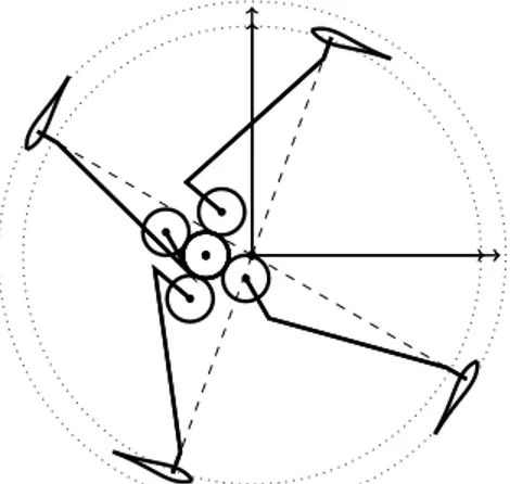
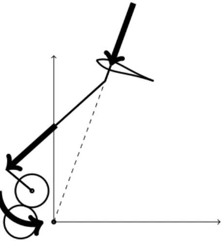
2.1.1 Purpose of the central gear eccentricity
A car engine is a ”rod-crank” system for which the piston has an alternat-ing translational movement. When the piston is at the top dead, the force is maximum and the torque produced is zero(5). The turbine is also a rotating rod-crank system for which the rotation center of the crank has an alternating translational movement. When the force is maximum and the torque produced is optimized(figure 4). With the eccentricity of the central gear, The trajectory of the blade follows almost the trajectory of a circle(figure 2), as for a Darrieus turbine [5]. The radial velocity of the profile is practically zero. Without eccen-tricity, this velocity isn’t zero and it is no longer negligible(figure 3).
Rmaxi f or β= 0 ou 180 degrees
Rmaxi(0 degrees) = − Ex+ 2 Rg+ Rb+ Ro+ Sl
Rmaxi(180 degrees) = − Ex− 2 Rg+ Rb− Ro− Sl
|Rmaxi(0 degrees)| = |Rmaxi(180 degrees)| => Ex = Rb (1)
With a mathematical approach R(β) = (Rb− Ex) cos(β) + 2Rg+ p R2 o− ((Rb+ Ex)sin(β))2+ Sl dR(β) dβ = (Rb− Ex)sin(β) − (Rb+ Ex)sin(β) pR2 o− ((Rb+ Ex)sin(β))2 dR(β) dβ → 0 when Rb = Ex (2) and (Rb+ Ex) Ro → 0 Ro >> (Rb+ Ex)
Figure 2: With the eccentricity
Figure 4: Active lift turbine : torque optimized
2.1.2 rapid and simplified calcul
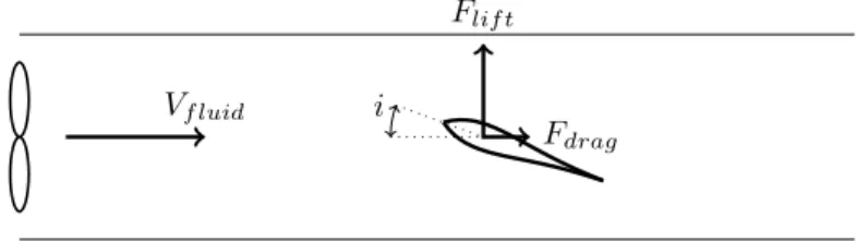
Lift force : Tunnel tests of the tunel profiles define the lift and drag co-efficient. For symmetric naca profiles type naca0012, with angles less than 13 degrees, the drag coefficient Cdis negligible and one can make an approximation
of the lift coefficient by this formula Cl≈ 0.1i (i : incidence angle in degrees).
For angles less than 13 degrees, it is considered that the force created by the fluid on the profil is perpendicular to the direction of the fluid and its value is:
F = 0.1i 1
2 ρ H C V
2 f luid
i: angle of incidence in degrees ρ: f luid density C: cord prof il H: height prof il Vf luid : f luid velocity
Flif t
Fdrag
i Vf luid
Figure 6: profil test
chord : According to the Betz theory, the fluid velocity at the turbine is Vf = 23Vf luid. [1]
The coefficient ’λ : tip speed ratio’ verify that the angle of incidence remains less than the maximum angle of incidence (13 degrees)
λ= ω R
Vf ω= 2 π 60 rpm 1
λ ≤ tan(10 degrees)
σis the stiffness coefficient. σ = numberbladeC R
In principle, the product σ λ must be less than 0.75. (σ ≤0.75
λ ) [6] [4]
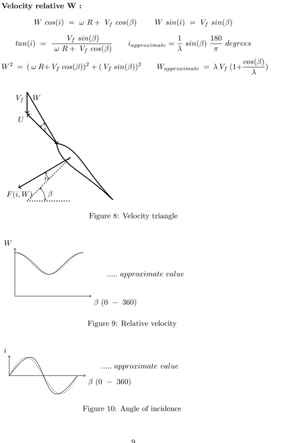
Velocity relative W :
W cos(i) = ω R + Vf cos(β) W sin(i) = Vf sin(β)
tan(i) = Vf sin(β) ω R+ Vf cos(β) iapproximate= 1 λ sin(β) 180 π degrees W2 = ( ω R+ Vf cos(β)) 2 + ( Vfsin(β)) 2 Wapproximate = λ Vf(1+ cos(β) λ ) U Vf W F(i, W ) i i β
Figure 8: Velocity triangle
W
β (0 − 360)
... approximate value
Figure 9: Relative velocity
i
β (0 − 360)
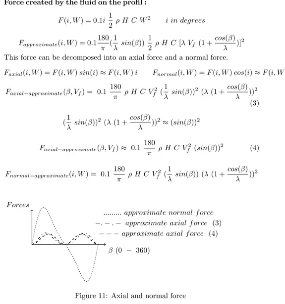
Force created by the fluid on the profil : F(i, W ) = 0.1i 1 2 ρ H C W 2 i in degrees Fapproximate(i, W ) = 0.1 180 π ( 1 λ sin(β)) 1 2 ρ H C [λ Vf (1 + cos(β) λ )] 2
This force can be decomposed into an axial force and a normal force.
Faxial(i, W ) = F (i, W ) sin(i) ≈ F (i, W ) i Fnormal(i, W ) = F (i, W ) cos(i) ≈ F (i, W )
Faxial−approximate(β, Vf) = 0.1 180 π ρ H C V 2 f ( 1 λ sin(β)) 2 (λ (1 +cos(β) λ )) 2 (3) (1 λ sin(β)) 2 (λ (1 +cos(β) λ )) 2 ≈ (sin(β))2 Faxial−approximate(β, Vf) ≈ 0.1 180 π ρ H C V 2 f (sin(β)) 2 (4) Fnormal−approximate(i, W ) = 0.1 180 π ρ H C V 2 f ( 1 λ sin(β)) (λ (1 + cos(β) λ )) 2 F orces β (0 − 360)
... approximate normal f orce −. − . − approximate axial f orce (3)
− − − approximate axial f orce (4)
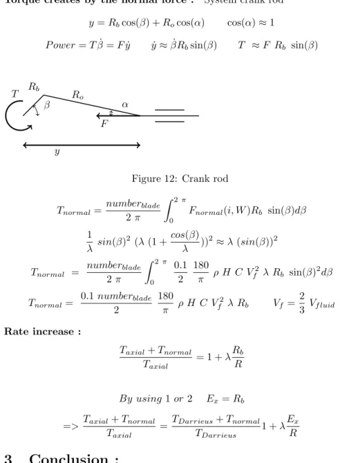
Torque creates by the normal force : System crank rod y= Rbcos(β) + Rocos(α) cos(α) ≈ 1
P ower= T ˙β= F ˙y ˙y ≈ ˙βRbsin(β) T ≈ F Rb sin(β)
Rb Ro F T y β α
Figure 12: Crank rod Tnormal=
numberblade
2 π
Z 2π
0
Fnormal(i, W )Rb sin(β)dβ
1 λ sin(β) 2 (λ (1 +cos(β) λ )) 2 ≈ λ (sin(β))2 Tnormal = numberblade 2 π Z 2π 0 0.1 2 180 π ρ H C V 2 f λ Rb sin(β) 2 dβ Tnormal= 0.1 numberblade 2 180 π ρ H C V 2 f λ Rb Vf = 2 3 Vf luid Rate increase : Taxial+ Tnormal Taxial = 1 + λRb R By using 1 or 2 Ex= Rb => Taxial+ Tnormal Taxial = TDarrieus+ Tnormal TDarrieus 1 + λEx R
3
Conclusion :
Although the calculation is simplistic, we find the same earnings as in the preprint[6]. The yield of active lift turbine is clearly increased by report a Darrieus turbine.
References
[1] Betz A. Das maximum der theoretisch moglichen ausnutzung des windes-durch windmotoren. Zeitschrift fur das gesamte Turbinenwesen, (26):307– 309, 1920.
[2] P. Lecanu J. Breard. Turbine telle qu’eolienne, en particulier a axe vertical, notamment de type darrieus. Brevet INPI, 2009. N et date de publication de la demande FR2919686 - 2009-02-06 (BOPI 2009-06).
[3] P. Lecanu J. Breard. Turbine telle qu’eolienne d’axe essentiellement vertical a portance active. Brevet INPI, July 2015. N et date de publication de la demande FR3016414 - 2015-07-17 (BOPI 2015-29).
[4] Ir M. Godard-Ing J. David-Ing G. Genon. Optimisation d’une eolienne dar-rieus a pales droites, analyse du couple de demarrage et realisation d’un pro-totype. ISILF Institus superieurs industriels libres francophones, 18, 2004. Gramme Liege.
[5] MARIE DARRIEUS GEORGES JEAN. Turbine a axe de rotation transver-sal a la direction du courant. Brevet INPI, May 1926. N et date de publica-tion de la demande FR604390 - 1926-05-03.
[6] Pierre normandajc Lecanu, Joel Breard, and Dominique Mouaz´e. Simplified theory of an active lift turbine with controlled displacement. working paper or preprint, April 2016.
[7] P. Lecanu J. Breard O. Sauton. Turbine a portance active a deplacement controle. Brevet INPI, June 2015. demande 1555859, soumission 1000299939.