HAL Id: hal-01672513
https://hal.archives-ouvertes.fr/hal-01672513
Submitted on 25 Dec 2017
HAL is a multi-disciplinary open access archive for the deposit and dissemination of sci-entific research documents, whether they are pub-lished or not. The documents may come from teaching and research institutions in France or abroad, or from public or private research centers.
L’archive ouverte pluridisciplinaire HAL, est destinée au dépôt et à la diffusion de documents scientifiques de niveau recherche, publiés ou non, émanant des établissements d’enseignement et de recherche français ou étrangers, des laboratoires publics ou privés.
medium-sized magnetic nanoparticles
H. Ezzaier, J. Alves Marins, I. Razvin, Micheline Abbas, A. Ben Haj Amara,
A. Zubarev, P. Kuzhir
To cite this version:
H. Ezzaier, J. Alves Marins, I. Razvin, Micheline Abbas, A. Ben Haj Amara, et al.. Two-stage kinetics of field-induced aggregation of medium-sized magnetic nanoparticles. Journal of Chemical Physics, American Institute of Physics, 2017, 146 (11), �10.1063/1.4977993�. �hal-01672513�
Two-stage kinetics of field-induced aggregation of medium-sized magnetic nanoparticles
H. Ezzaier1,2, J. Alves Marins1, I. Razvin1, M. Abbas3, A. Ben Haj Amara2, A. Zubarev4, and P.Kuzhir1,*
1 University Côte d’Azur, CNRS UMR 7010 Institute of Physics of Nice, Parc Valrose, Nice 06100, France 2Laboratory of Physics of Lamellar Materials and Hybrid Nano-Materials, Faculty of Sciences of Bizerte,
University of Carthage, 7021 Zarzouna, Tunisia,
3Laboratoire de Génie Chimique, Université de Toulouse, CNRS-INPT-UPS, Allée Emile Monso, 31030 Toulouse,
France
4Urals Federal University, Department of Mathematical Physics, Lenina Ave 51, 620083 Ekaterinburg,
Russia
Abstract
The present paper is focused on theoretical and experimental study of the kinetics of field-induced aggregation of magnetic nanoparticles of a size range of 20-100 nm. Our results demonstrate that (a) in polydisperse suspensions, the largest particles could play a role of the centers of nucleation for smaller particles during the earliest heterogeneous nucleation stage; (b) an intermediate stage of the aggregate growth (due to diffusion and migration of individual nanoparticles towards the aggregates) is weakly influenced by the magnetic field strength; (c) the stage of direct coalescence of drop-like aggregates (occurring under magnetic attraction between them) plays a dominant role at the intermediate and late stages of the phase separation, with the timescale decreasing as a square of the aggregate magnetization.
I. Introduction
Magnetic micro- and nanoparticles and their liquid suspensions or gels are gaining a growing interest in environmental and biomedical applications, such as water purification from organic and inorganic molecules1,2, magnetic resonance imaging3,4, cell separation5, protein purification6,7, magnetic hyperthermia8,9, controlled drug delivery and release10,11, magneto-mechanical lysis of tumor cells12,13, high sensitivity immunoassays14 and tissue engineering15,16. In many of these applications, magnetic particles are subject to aggregation induced by an external applied magnetic field, and the kinetics of aggregation becomes an important factor affecting efficiency of a considered system. An excellent example is enhancement of the magnetophoresis of magnetic microbeads due to their field-induced aggregation – the phenomenon referred to as cooperative magnetophoresis17-20, which could be beneficial for separation and detection of biomolecules using functionalized magnetic microbeads.
Most of existing works characterize the field-induced particle aggregation in terms of three governing parameters – the particle volume fraction , the ratio of the energy of dipole-dipole interaction between particles to thermal energy – so called dipolar coupling parameter and the ratio of the energy of interaction of a magnetic particle with an external magnetic field of an intensity H0 to thermal energy called magnetic field parameter or Langevin parameter . Both
2 3 3 0 4 p B m d k Td , (1a) 0 3 p B m H d k T , (1b)
where0=410-7 H/m is the magnetic permeability of vacuum; mp - the particle magnetic
moment (in T×m3); d – its diameter, kB≈1.38×10⁻²³ J/K - the Boltzmann constant and T –
absolute temperature. Since the particle magnetic moment is linear with the particle volume, the parameters and are proportional to the cube of the particle size. The physics of particle aggregation is rather different for micron-sized particles (with >>1) and for nanoparticles (with1).
Kinetics of field-induced aggregation of micron or sub-micron-sized particles (typically d>100 nm) has been studied experimentally by either direct visualization22-24 or light scattering
25-28
. The common feature shared between most of the studied systems is that these particles exhibit a rapid field-induced aggregation in linear chains aligned with the direction of applied magnetic field, and the average chain length 2a grows with time as 2a t, with 0.45 0.8. At longer times, lateral aggregation dominates over tip-to-tip aggregation and the chains can merge and form either a fibrous structure “frozen” in non-equilibrium state likely by inter-particle friction22 or column structures confined by the walls orthogonal to the applied field29, or unconfined ellipsoidal drop-like aggregates under pulsed magnetic field30,31. Theoretical studies are mainly based on Langevin dynamics simulations19,32,33 or solution of Smoluchowsky kinetic equation 23,24,27,28,33-35. A simplified theoretical approach, so-called hierarchical model, has been developed by See and Doi36 considering only coalescence of the chains of equal sizes and showing a satisfactory agreement with experiments on 2a , even though it predicts monodisperse particle chains instead of experimentally observed polydisperse distribution.
In the opposite size limit, typically d<20 nm, when considering aggregation, one usually speaks about field-induced phase separation or a condensation phase transition. Appropriate phase diagrams and equilibrium microstructures have been extensively studied theoretically and experimentally37-47. Kinetics of phase separation has been studied by light scattering by Socoliuc and Bica48 for aqueous dispersions of nanoparticles (ferrofluids) and by Laskar et al.49 for non-aqueous ferrofluids. Elongated scattered patterns have been reported by these authors corresponding to formation of long drop-like aggregates, which during time settle to a stable space configuration owing to magnetic lateral repulsion. Thermodynamic approach broadly used for molecular liquids is appropriate for modeling of the phase separation in suspensions of magnetic nanoparticles. Using this approach, Zubarev and Ivanov50 and Ivanov and Zubarev51 have considered three different stages of the phase separation: (a) appearance of critical nuclei at early stage of homogeneous nucleation; (b) evolution of the nuclei to long drop-like aggregates, and (c) Oswald ripening when the particles are transferred from smaller to larger aggregates leading at infinite times to a full coalescence of the concentrated phase into a single bulk phase. The aggregate size distribution has been calculated and the average aggregate volume has been
found to increase with time as 7 / 4
V t at early stage, followed by an intermediate plateau at the end of the stage (b) showing a final increase with V t7 / 6at the ripening stage (c).
Magnetic nanoparticles of medium size, 20<d<100 nm have not been available for a long time because of difficulties related to their colloidal stabilization. To prevent their aggregation by magnetic interactions in zero field, they have to be superparamagnetic. So, these particles are usually porous nanoclusters composed of smaller 10-nm superparamagnetic nanoparticles52-56. Similarly to small nanoparticles, medium-sized colloids exhibit condensation phase transitions54,55,57 which enhance drastically their magnetic separation on magnetized collectors
57-61
. Kinetics of phase separation of medium-sized nanoparticles has been studied only scarcely. Socoliuc et al.54 has conducted direct visualization and light scattering experiments on 80-nm magnetic nanoclusters and shown appearance of elongated drop-like aggregates. In addition to three kinetic stages postulated by Zubarev and Ivanov50 and Ivanov and Zubarev51, Socoliuc et al.54 claims a forth final stage of coalescence of aggregates into larger domains. This kinetics seems to combine features of condensation phase transitions of small nanoparticles with aggregation of large micron- or submicron-sized particles. To the best of our knowledge, theoretical description of such kinetics is still missing.
The present paper is focused on theoretical modeling of kinetics of aggregation (or phase separation) of the medium-sized (20<d<100 nm) superparamagnetic nanoparticles. The main goal is to establish theoretical correlations for the temporal evolution of the aggregate size and shape as function of the initial supersaturation of the suspension (or initial particle volume fraction 0) and of the applied magnetic field. To check our model, aggregation process is
visualized using an optical microscope and the size and shape of the aggregates is analyzed as function of time. Visualization experiments allow assessing dominant mechanisms of aggregation, which are implemented into the theory. Therefore, the present theory is developed for two stages that are explicitly distinguished in our experiments and are interesting from the practical point of view: (a) intermediate aggregate growth by particle diffusion and magnetophoresis, and (b) aggregate coalescence due to dipolar interactions. Simple hierarchical model of See and Doi36 developed for chain-like clusters is extended to coalescence of drop-like aggregates, while the transition between two aggregation stages is managed by comparison of the aggregation rates at each stage.
The present paper is organized as follows. Theoretical model implying two observed aggregation stages is developed in Sec. II. The aggregate growth and coalescence stages are described in Secs. II-A and II-B, respectively, while the transition between stages is considered in Sec. II-C. Experimental details of optical visualization and image processing are provided in Sec. III. Experimental data on temporal evolution of the aggregate size are compared with theoretical results in Sec. IV, while the conclusions and perspectives are outlined in Sec. V.
II. Theory
A. Aggregate growth
Let us consider initially homogeneous suspension of Brownian super-paramagnetic hard sphere particles, all having the same diameter d, and dispersed at a volume fraction 0 in a
particles magnetic moment is zero, they do not exhibit dipolar interactions and do not form any clusters.
When a uniform external magnetic field, of intensity H0, is applied, particles acquire
magnetic moments and attract to each other, while the Brownian motion tends to re-disperse them. Depending on the values of 0 and H0, the suspension undergoes a phase separation
manifested by appearance of elongated aggregates. At infinite times the systems tends to a thermodynamic equilibrium at which the particle volume fraction in the dilute (outside the aggregates) and concentrated (inside the aggregates) phases tend to steady-state values ' and
''
depending on H0, while '(H0) and
''(H0) dependences correspond to coexistence curvesof a 0- phase diagram38. Such diagrams have been modeled for our particular nanocluster
suspensions55,57, and strong inequality ''' has been found. In the present paper, ' is directly measured as function of H0 [see figure 6 in Sec. IV-A], while the value ''0.6 close to
the random close packing limit is taken for the aggregates. In this section, we intend to find the evolution of the aggregate size and shape with time and as a function of two governing dimensionless parameters 0 0 ' called initial supersaturation62 and - the magnetic field parameter depending on H0 [Eqs. (1b), (10)].
The aggregation starts by a short nucleation stage not considered here, which is most likely heterogeneous and during which primary aggregates composed of large number of particles are expected to appear around the biggest particles playing a role of nucleation centers. These primary aggregates are supposed to be of the same size and to have a shape modeled by a prolate ellipsoid of revolution extended along the applied magnetic field as commonly admitted in theoretical models30,50,51 and observed in experiments with ferrofluids48,54,63-65. Initial volume V0 and initial volume fraction 0 of primary aggregates (ratio of the total volume of all the
aggregates to the suspension volume) are considered as adjustable parameters of the model. During time, individual magnetic particles of the dilute phase surrounding the aggregates are attracted to the aggregates and induce the aggregate growth. The aggregates are supposed to conserve their ellipsoidal shape but their concentration in the suspension and size, characterized by a major semi-axis a, a minor semi-axis b (as depicted in Fig. 1) and a volume
2
4 / 3
V ab , increase progressively with time. Nevertheless, the aggregate concentration is supposed to remain low enough <<1 (approximation valid for very dilute suspensions with
0/'' 1
), and possible coalescence of aggregates at this stage is neglected. The aggregate shape is quantified by their aspect ratio ra=a/b, which is assumed to be very high, ra>>1, in
agreement with numerous observations48,54,63-65. During all this aggregation stage, the aggregates are supposed to be of equal size, their number concentration is assumed to be constant with time
0 0
/ /
n V V , while possible appearance of new nuclei is neglected. These rough approximations are to some extent supported by the more precise theory of aggregation of small nanoparticles50 (d<20 nm).
Fig.1. Sketch of the ellipsoidal aggregate. Cylindrical and ellipsoidal coordinates are introduced. Key values of the particle concentration inside the aggregate (”), on the outer side of the aggregate surface (’) and far from the
aggregate () are also indicated. The external uniform magnetic field H0 is oriented along the z-axis. The internal aggregate volume fraction i (ratio of volumes of all particles constituting
the aggregate to the aggregate volume) is supposed to be close to the equilibrium concentration of the concentrated phase: i ''0.6, while the particle concentration in any point of the dilute phase around the aggregate is i. Finally, possible sedimentation of individual particles and aggregates is neglected. This assumption is justified in Sec. III.
The starting point of the model is the particle conservation equation implying that the growth rate, dN/dt of the number of particles, N, in the aggregate is equal to the particle flux J towards the aggregate:
(ni n dVs) '' dN dV J dt dt v dt , (2)
whereni i/v''/v is the number concentration of particles inside the aggregates; ns s /v
and sare respectively the number concentration and the volume concentration of individual particles around the aggregate in the vicinity of its surface; v is the volume of primary particles.
The particle flux density j outside the aggregates at any point of the dilute phase is related to the gradient of the local chemical potential and local volume fraction of particles. The expressions for and j take the following form in the dilute-limit approximation50,66:
ln ln u B B k T U k T e , (3a)
u u D e e v v j , (3b)where and Dk TB k TB /(30d) are the particle mobility and diffusion coefficient, respectively; U and uU/(k TB ) are respectively the dimensional and dimensionless energies of magnetic interaction of a particle with the local field H at a given position of the particle outside the aggregate. The expression for U takes the following form under the approximation of linear magnetization of particles, valid at low magnetic field intensities H04 kA/m, considered in our
experiments67: 2 0 3 2 p p U
m dH H v, (4)where p p/(3p) is the magnetic contrast factor of an individual nanoparticle of a
magnetic susceptibility p. The spatial distribution of the magnetic field H around the ellipsoidal
aggregate and the dimensionless energy u are calculated in Appendix A.
Let us introduce axisymmetric ellipsoidal coordinate system (, , ), with an origin situated at the aggregate center and whose coordinate surfaces =const and =const represent confocal ellipsoids of revolution and hyperboloids of revolution, respectively [Fig. 1]. These coordinates are related to the coordinates (, , z) of the cylindrical coordinate system by the following expressions68:
zc; 2c2(21)(12); s 1; 1
1, (5) where c2 a2b2 and s a c/ is the value of on the aggregate surface. The polar coordinate is common for both coordinate systems. The metric coefficients of the ellipsoidal system are2 2 2 2 1 g c ; 2 2 2 2 1 g c ; 2 2 2 ( 1)(1 ) g c . (6)
The particle diffusion towards the aggregates is considered in quasi-stationary approximation divj0, for which it can be shown that (a) the particle flux J through the surfaces =const is independent of ; (b) the chemical potential of particles outside the aggregates depends only on the coordinate , and (c) the product u
e
intervening into Eq. (3b) is independent of . Bearing this in mind, we arrive at the following expressions for the normal component of the particle flux density and the flux through a coordinate surface =const:
1 u u D j e e v g , (7a)
1 1 2 0 1 1 2 D ( 1) u u J j dS j g g d d c e e d v
, (7b)where we make use of Eq. (6) for the metric factors and the minus sign in Eq. (7b) comes from the fact that the particle flux is the oriented towards the aggregate. Isolating the term
eu /, and integrating over from s to infinity, we get the following expression for the particle flux
0 1 1 2 1 2 ( 1) s S u u s u e e D J c v e d d
. (8)Here u0 is the dimensionless energy of the particle in the external filed H0, is the particle
volume fraction at the infinite distance from the aggregate, us and s are respectively the
dimensionless energy and concentration of particles at any point (s, ) situated on the outer side
of the aggregate surface. Since the product us
se
is independent of , it can be replaced by 0
0
u s e
, where s0 is the particle concentration at the point of the aggregate surface where the magnetic field intensity is equal to H0. Furthermore, the local thermodynamic equilibrium at the aggregate
surface imposes that the concentration outside and inside the aggregate are approximately equal to the binodal concentrations: s0 'and i '' [Fig. 1]. This allows expressing the particle flux through the supersaturation ' of the suspension:
2 D
J c
v I
, (9)
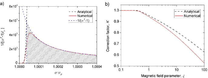
where the integral 0
1 1 ( ) 2 1 ( 1) S u u I e d d
is estimated in Appendix B [cf. Eq. (B-6)] as a function of the magnetic field parameter [Eq. (1b)], which, for the case of the medium-sized magnetic nanoparticles with induced dipole moment and linear magnetization appears to be proportional to the square of the magnetic field intensity H0 and takes the following form:2 0 0 0 3 2 p B H v u k T . (10)
In the aforementioned case, the parameter is closely related to the dipolar coupling parameter [Eq. (1a)] through: p / 4 . In the considered limit of high aspect ratio aggregates, ra=a/b>>1, the magnitude c intervening into Eq. (9) could be expressed through the aggregate
volume V ab2/ 3: 1/ 3 2 2 1/ 2 3 2 ( ) a c a b a Vr . (11)
On the other hand, the local thermodynamic equilibrium of an aggregate requires the minimization of its free energy at any time and leads to the following key relationship50 between the aggregate volume V and its aspect ratio ra valid at ra>>1:
7 3 ln a a r V B r ; 3 4 2 0 48 B M , (12)
where M is the aggregate magnetization and – the aggregate surface tension. The volume-scale B has been shown to be of the order of particle volume69: B3v/ 64. Equation (12) allows expressing lnra and ra through V using the strong inequality ln(ln )ra lnra valid at ra>>1:
1 ln ln 7 a V r B , (13a) 1/ 7 1/ 7 3/ 7 3/ 7 1 ln ln 7 a a V V V r r B B B . (13b)
Combining together Eqs. (2), (9), (11), (13) and (B-6), equation (2) of the aggregate growth takes the following form:
3/ 7 1/ 3 5/ 7 / 4 '' ln ( / ) V B dV DB dt K V B , (14) where 5/ 7
1/ 3 7 / 3 2.5 and K is a numerical factor depending on and given by Eq. (B-6b) in Appendix B.
To integrate Eq. (14), we need to relate the supersaturation ' to the aggregate volume V. First, the concentration can be estimated from the condition of conservation of the total volume of particles in the suspension:
0 i (1 )
, (15)
with i ''. Second, under the aforementioned assumption of a constant number of aggregates during the aggregate growth stage, (n /V const 0/V0), the aggregate concentration at a given time t is related to the aggregate initial volume V0 and concentration 0 by
0 0
V V
. (16)
Combining Eqs. (15) and (16), and taking into account the smallness of the aggregate concentration, <<1, in initially dilute suspension with 0<<1, we obtain:
0 0 0 0 '' ' ' '' 1 V V . (17)
Recall that 0 0 ' is the initial supersaturation. The time integration of Eq. (14) with the initial condition V(0)=V0 leads to the following expression for the elapsed time t as function of
the dimensionless volumes Vˆ V B/ and Vˆ0 V0/B:
0 1 ˆ 2 / 3 3/ 7 0 0 5/ 7 ˆ 0 ˆ ˆ '' ˆ '' ˆ ˆ 4 (ln ) V V K B V V t dV D V V
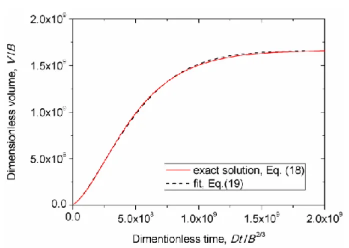
. (18)One can fit Eq. (18) by the following formula, exact at both short and long time limits:
2 / 3 5/ 7 0 3/ 7 0 ˆ (ln )ˆ ln ˆ 4 I I V K B V t f D V , (19-a)
0.45 0.3 1 0.8 1 I I I f , (19-b)
where I 0 ''0 is the suspension supersaturation at the beginning of the aggregate growth stage corresponding to primary aggregates with a volume V0. Both theoretical dependencies (18)
and (19) of the dimensionless volume VˆV B/ on the dimensionless time tˆDt B/ 2/ 3 are plotted in Fig. 2 for the following values of the parameters appropriate for our experimental conditions: 4 0 10 , 6 0 10 , ''0.6, Vˆ0 107, K1.
Fig. 2. Theoretical dependence of the dimensionless aggregate volume on the dimensionless time for the aggregate growth stage. The following set of parameters were used in calculations: 0 104, 6
0 10 , ''0.6, 7 0 ˆ 10 V , K1.
The aggregate volume exhibits an initial sharp increase with time and becomes almost constant at longer times. Such saturation of the aggregate volume corresponds to the vanishing of the suspension supersaturation [Eq. (17)] with time when the dilute phase concentration approaches the binodal concentration ' and the aggregate concentration tends to its maximum value dictated by particle conservation [Eq. (15)]: m 0/''1. However, such a state with a final number of aggregates, n 0/V0, is thermodynamically unfavorable, since aggregates start to coalesce in order to decrease the suspension free energy – the mechanism considered in Sec. II-B. Another striking point is that the characteristic time of the aggregate growth is about nine orders of magnitude higher than the diffusion timescale t B2 / 3/D d2/D at the considered set of parameters. This is explained by the fact that the aggregates contain a very large number of particles (107-109 in the current example), and the real time scale is based on the aggregate volume, rather than on the particle volume, as inferred from Eq. (19): t
2 / 3 4 / 7
0 ˆ
(B /D V)( m / ).
Finally, the considered kinetics includes both diffusive and magnetophoretic particle fluxes related respectively to the 1st and the 2nd term of Eq. (3a) for the chemical potential. The diffusive flux arises thanks to the fact that the particle concentration in the dilute phase in the vicinity of the aggregate surface is close to the equilibrium value ' and is lower than the concentration far from the aggregate. The magnetophoretic flux is responsible for particle
migration towards the aggregate due to magnetic attraction. The contribution of magnetophoretic flux appears in final equations (18) and (19) through the numerical multiplier K1, which is logarithmically decreasing function of the magnetic field parameter [cf. Eq. (B-6b) in Appendix B]. The magnetophoretic flux (or the value of K) does not change the shape of the time dependency of the aggregate volume [Fig. 2] but decreases the time of the aggregate growth, with respect to the time governed exclusively by diffusive flux.
B. Aggregate coalescence
As already pointed out, the state with a finite number of aggregates is thermodynamically unfavorable, the system tends to decrease the surface area between concentrated and dilute phases, which promotes coalescence of aggregates, even if their concentration is low. In the present section, we consider the coalescence stage of the phase separation neglecting possible aggregate growth by absorption of individual particles from the dilute phase. This assumption is valid if the timescale of the aggregate growth stage is much shorter than that of the coalescence stage, such that the dilute phase concentration rapidly approaches the binodal concentration
'
and the aggregates no more able to absorb particles from the surrounding fluid. The coalescence is supposed to begin when the aggregates achieve some initial volume V, same for all of them, and initial volume fraction , which can be different from those used for the initial conditions of the aggregate growth stage [Sec. II-A]. Again, during all this stage, the aggregates are assumed to preserve their ellipsoidal shape, high aspect ratio ra>>1, low concentration <<1
and to be of the same size. We seek for the evolution of the aggregate volume with time thanks to their coalescence induced by magnetic attraction between them.
To this purpose, we adopt the basic idea of the hierarchical model of See and Doi36, who considered that all pairs of primary aggregates coalesce at the same time producing secondary aggregates of a volume 2V, then, all the pairs of secondary aggregates coalesce at the same time into the aggregates of a volume 4V, and so on, until full coalescence of the bulk concentrated phase. At the beginning of the coalescence stage (t=0), the initial number fraction of aggregates is n /V. Let 0 be the time for two neighboring aggregates to coalesce into an aggregate of
a volume V1 2V . The number concentration of the aggregates at t=0 is divided by two, 1 / 2
n n , while the volume fraction does not change, 1 under considered assumption that the aggregate do not absorb individual particles from the surrounding fluid. After the first coalescence, the secondary aggregates will coalesce into aggregates of a volume 2
2 2 1 2
V V V
at number fraction 2 2 / 2
n n during a time interval 1. The i-th coalescence step will
correspond to the aggregate volume Vk 2kV, the number fraction / 2 k k
n n and the volume fraction k , while the total elapsed time from the beginning of the process is
1 0 k k i i t
. We have now to relate the time interval i of each i-th coalescence step to theaggregate volume Vi.
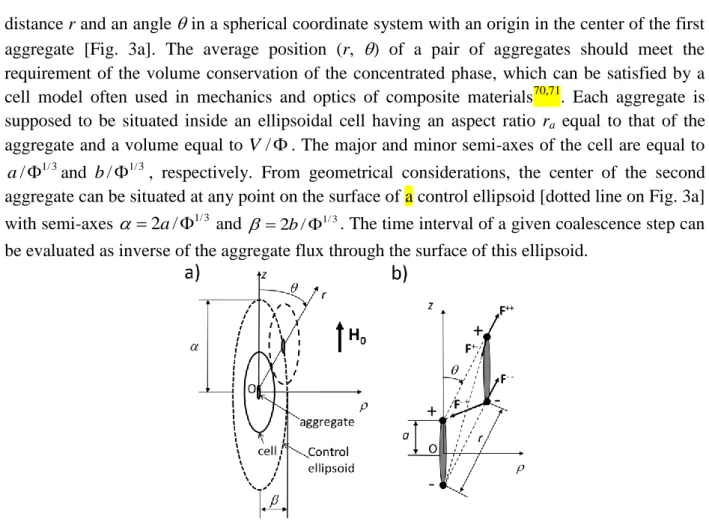
To this purpose, let us consider two identical drop-like aggregates aligned with the applied magnetic field and having a major semi-axis a, a minor semi-axis b, an aspect ratio ra=a/b>>1 and a volume V 4ab2/ 3. Mutual position of their centers is described by a
distance r and an angle in a spherical coordinate system with an origin in the center of the first aggregate [Fig. 3a]. The average position (r, ) of a pair of aggregates should meet the requirement of the volume conservation of the concentrated phase, which can be satisfied by a cell model often used in mechanics and optics of composite materials70,71. Each aggregate is supposed to be situated inside an ellipsoidal cell having an aspect ratio ra equal to that of the
aggregate and a volume equal to V/. The major and minor semi-axes of the cell are equal to
1/ 3
/
a and b/1/ 3, respectively. From geometrical considerations, the center of the second aggregate can be situated at any point on the surface of a control ellipsoid [dotted line on Fig. 3a] with semi-axes 2 /a 1/ 3 and 1/ 3
2 /b
. The time interval of a given coalescence step can be evaluated as inverse of the aggregate flux through the surface of this ellipsoid.
Fig. 3. Sketches of the cell model (a) and of the “four charges” model (b). In both cases, the external uniform magnetic field H0 is oriented along the z-axis
During the coalescence stage, the aggregates have a size of several microns and their diffusive flux is therefore negligible. The magnetophoretic flux of the aggregates through the surface of the control ellipsoid is expressed through the force F of magnetic interactions between two aggregates as follows:
II
0 0 0 2 ( ) 2 2 z z J J J J n dS n F n dS n F n dS
ζ F n
, (20)wheren /V is the aggregate number fraction supposed to be homogeneous on the aggregate surface;n is the outward unit vector normal to the control ellipsoid surface; , II are the
transverse and longitudinal diagonal components of the aggregate mobility tensor ζ . The two terms in the right-hand side of Eq. (20) correspond to the radial and axial components of the flux with respect to the cylindrical coordinate system (, , z) introduced in Fig. 3a. The factor 2 before the integrals comes from the fact that both aggregates are moving towards each other at the same speeds, while the minus sign stands for the positive inward flux. The integration domain J>0 corresponds to the fact that only inward flux is considered to contribute to the coalescence of a given pair of aggregates, while the outward flux would induce a coalescence of another pair. The products n dS and n dSz are the projections of the surface element dS on the
z- and r- coordinate surfaces, respectively. They have the following expression in cylindrical coordinates:n dS 2( )z dzand n dSz 2 d , where
2 2 1/ 2 ( )z ( z ) /ra
on the control ellipsoid surface. The expression (20) for the flux reads:
0 0 II 0 2 4 ( ) 4 z z J n F z dz n F d
, (21)where (0, z0) are the coordinates of the point on the control ellipsoid surface where the flux
density is zero.
The magnetic force F will be estimated in a “four charges” approximation initially developed for chains of magnetic particles29. By analogy with electrostatics, the induced dipole moment of each aggregate is supposed to be a result of two opposite point charges q and –q concentrated at the aggregate tips, as shown schematically in Fig. 3b. The charge q is related to the aggregate dipole moment ma 2aq , and the latter is defined though the aggregate magnetization M as ma 0MV, such that q0MV/(2 )a . Absolute values of the four forces acting on the poles of the right aggregate in Fig. 3b are given by the Coulomb’s law, neglecting magnetic susceptibility of the medium surrounding the aggregates:
2 2 0 4 q F F r ; 2 2 0 1 4 q F r ; 2 2 0 2 4 q F r , (22) where r2 2z2, 2 2 2 1 1 r z and 2 2 2 2 2
r z are the squares of the distances between different pairs of charges belonging to two aggregates; r corresponds to the distance between the centers of two aggregates; z1 z 2a and z2 z 2a. The radial and axial components of the total force acting on the right aggregate of Fig. 3 read:
2
1 2 3 3 3
0 1 2
2 1 1
( ) sin sin sin
4 q F F F F F r r r ; (23-a) 2 1 2 1 2 3 3 3 0 1 2 2
( ) cos cos cos
4 z z z q z F F F F F r r r , (23-b)
Where , 1 and 2 are the angles between the z-axis and the lines connecting different pairs of
charges belonging to two aggregates; corresponds to the angle that the line connecting the aggregate centers makes with the z-axis.
Evaluation of the flux [Eq. (21)] with appropriate expressions for the forces F, Fz and
for the charge q shows that the second term (axial flux) is always negligible under considered approximations <<1, ra>>1, while the first term (radial flux) reads:
0 2 2 0 2 3/ 2 3/ 2 3/ 2 2 2 2 2 2 2 2 2 2 2 2 2 2 0 2 2 ( 1) ( 2 ) ( 2 ) ( ) a z a a a n M V J r a r z z r z a z r z a z dz
. (24)Estimation of this integral is presented in detail in Appendix C, and the final result for the aggregate flux reads:
1 2 0 2 2 / 3 2 0 ln 25 5 1 6 24 a a a M r J r r . (25)
The aggregate aspect ratio ra and its logarithm are related to the aggregate volume by Eqs. (13),
therefore the time interval of the i-th coalescence step is related to the volume Vi, as follows:
1/ 7 2 / 7 1 * 1/ 7 7 ( / ) 7 ln( / ) ln ( / ) i i i i i V B J V B V B (26) where 25 5 /(242 / 3) and * 2 0 0 6 /( M )
is a characteristic timescale of the coalescence stage with the aggregate magnetization, M, independent of ra and Vi thanks to
negligible demagnetizing effects in the high aspect ratio limit, ra>>1. The total elapsed time
corresponding to k successive coalescence steps is obtained by summing up the durations i and
using 2i i V V: 1/ 7 2 / 7 1 1 * 1/ 7 0 0 ˆ 7 (2 ) 7 ˆ ˆ ln(2 ) ln (2 ) i k k k i i i i i V t V V
, (27)where Vˆ V /B and B
3v/ 64 as it was defined below Eq. (12), v is the volume of individualnanoparticle. The sum in Eq. (27) admits the following approximate expression with a maximal deviation of 3.7% from the exact numerical result:
1/ 7 2 / 7 2 / 7 * 2 / 7 1/ 7 1 ˆ ˆ ln(2 ) 7 7 2 1 ln ˆ ˆ ln 2 ln ln (2 ) 2 1 k k k k V V t V V . (28)
Finally, using 2k Vk/V in the last equation, and moving form a discrete variation of the
volume to a continuous variation, valid at k>>1 (omitting subscripts k at Vk and tk), we get the
following expression for the elapsed time t as function of the dimensionless volume ˆV V B/ :
2 / 7 2 / 7 1/ 7 * 2 / 7 1/ 7 ˆ ˆ ˆ 7 ln 7 ln ˆ ˆ ln 2 ln 2 1 ln V V V t V V (29)
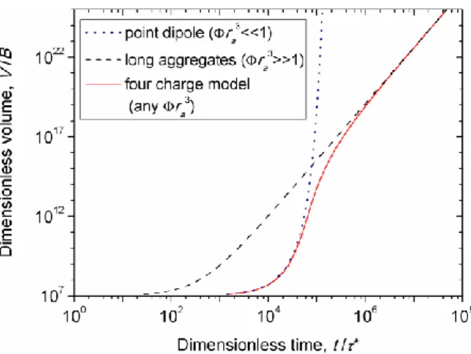
Theoretical dependency of the dimensionless aggregate volume ˆV on the dimensionless elapsed time tˆt/* is plotted in double logarithmic scale in Fig. 4 for the values =104 and
7
ˆ 10
V typical for our experiments.
The solid curve in that figure corresponds to the general expression Eq. (29) derived for any value of the parameter 3
a
r but in the limits <<1 and ra>>1. The shape of this curve is
explained by the behavior of two terms of Eq. (29). The first term in the brackets of Eq. (29) is dominant in the beginning of the coalescence process when the aggregates are still small enough and the strong inequality 3
1 a
r holds. This term corresponds to the point dipole approximation and gives an initial very slow linear increase of the aggregate volume
* (1 ln 2 /(7 ) ( / ))
V V t at t/*7 / ln 2 105, followed by an extremely fast growth
with time exp(ln 2 /(7 )t/ *)
V V at t/*7 / ln 2 10 5. However, at longer times, the aggregates become very long and the second term of Eq. (29) becomes dominant when the distance between aggregates is much shorter than their length, implying the strong inequality 3
1 a
r .This
second term gives a power-law growth of the aggregate volume with time, V * 7 / 2 ( / )
V t at
* 5
/ 7 / ln 2 10
t , explaining a final linear part of the V tˆ ˆ( ) dependency with a slope 7/2 in double logarithmic scale. Both asymptotic behaviors at 3
1 a
r and ra3 1corresponding to
two terms of Eq. (29) are shown in Fig. 4 by dotted and dashed lines, respectively.
Fig. 4. Theoretical dependences of the dimensionless aggregate volume on the dimensionless time for the aggregate coalescence stage. The following parameters were used in calculations:Vˆ 107, 104.
C. Transition between growth and coalescence stages
The transition from the aggregate growth stage (at shorter times) to the coalescence stage (at longer times) could be found by a simple approach based on comparison of aggregation rates, dV/dt, of both stages. The transition is supposed to take place at some volume V corresponding to the equality of the aggregation rates of two stages; the aggregate growth takes place at V<V and coalescence – at V>V. The aggregation rate for the growth stage is directly given by Eq. (14), while the rate for the coalescence stage is obtained by derivation of Eq. (29) with respect to
ˆ
V :
1
ˆ/ / ˆ
dV dt dt dV . The equality of aggregation rates gives the following transcendent equation for the dimensionless transition volume Vˆ:
1 3/ 7 6 / 7 0 0 2 / 3 5/ 7 * 2 / 7 5/ 7 1/ 7 0 ˆ ˆ 4 1 7 1 2 7 1 '' ˆ ˆ ˆ ˆ ˆ ˆ '' (ln ) ln 2 ln 2 1 ln V V D K B V V V V V V , (30)
recalling that the correction factor K is given as function of the magnetic field parameter by Eq.
(B-6b) in Appendix B and * 2 2
0 0 0 0ˆ 0
6 /( M ) 6 /( V M )
.
Once the value of Vˆ is obtained from numerical solution of Eq. (30), the elapsed time covering both phase separation stages is obtained from Eqs. (19) and (29) taking into account
that the initial time of the coalescence stage corresponds to the final time of the growth stage at ˆ ˆ V V: 2 / 3 5 / 7 0 3/ 7 0 5 / 7 2 / 7 2 / 7 2 / 3 1/ 7 * 0 2 / 7 3/ 7 1/ 7 0 ˆ (ln )ˆ ˆ ˆ ln , ; ˆ 4 ˆ (ln ˆ ) 7 ln ˆ 7 ˆ ˆ ˆ ˆ ln ln , , ˆ ˆ ˆ 4 ln 2 ln 2 1 ln I I I I V K B V f V V D V t V V V V K B V f V V D V V V (31)
where I 0 ''0 , 0 ''0V Vˆ / ˆ0 , 0 ''0V Vˆ ˆ/ 0 [Eq. (17)], and the
correction factor f
/ I
is given by Eq. (19-b).The behavior of Eq. (31) is inspected in details in Sec. IV, in which it is tested against experimental results, and the validity and drawbacks of the current approach (based on comparison of aggregation rates) are discussed.
III. Experiments
In experiments, the phase separation process was visualized using an optical microscopy. The main goal was to determine the aggregate size as function of the elapsed time, the magnetic field intensity and the initial particle volume fraction.
A suspension (ferrofluid) of iron-oxide nanoparticles dispersed in distilled water and covered by a double layer of oleate salts has been synthesized using a conventional method of co-precipitation of iron salts in alkali medium21,72. This synthesis gave permanent nanoclusters of nearly spherical shape and composed of numerous nanoparticles likely because of a rapid and uncontrolled kinetics of adsorption the second oleate layer55. The nanoclusters have a relatively broad size distribution ranging from 20 to 220 nm with the average size equal to 54 nm, as inferred from dynamic light scattering [Fig. S1 in Supplementary Material]. This size corresponds to the gravitational Péclet number 3 105
G
Pe , defined as the ratio of the diffusion time to the sedimentation time, and confirming a good stability of the suspension against gravitational sedimentation. The saturation magnetization of the solid phase of nanoclusters was measured by vibrating sample magnetometry and found to be MS=481 kA/m,
the value closed to that of the bulk magnetite. The details of the nanoclusters’ synthesis and characterization are given in Supplementary Material. To avoid any confusion between nanoclusters and aggregates, the former are hereinafter called magnetic particles or shortly particles.
The minimum particle volume fraction
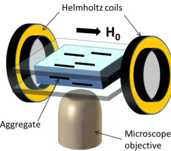
'at which the suspension undergoes phase separation at a given magnetic field was measured by direct visualization of the suspension structure. To this purpose, the synthesized ferrofluid was diluted by distilled water at different particle volume fractions ranging from 810-6 to 310-3 (810-4 – 0.3%vol.). Each suspension was injected to a transparent cell of a size 20100.2 mm sketched in Fig. 5 and formed by a Plexiglas substrate and a microscope glass slide separated from each other by a polyvinyl seal. The cell was placed into a transmitted light inverted microscope Nikon Diaphot-TMD (Japan) equipped with a complementary metal oxide semiconductor (CMOS) camera PixeLINKPL-B742U (Canada). An external homogeneous magnetic field was generated by a pair of Helmholtz coils placed around the microscope and was applied parallel to the thin layer of the suspension inside the cell. The observation of the suspension structure was carried out using a 50-fold objective (Olympus LMPlanFl 50×0.50) with a large working distance, allowing detection of aggregates of a minimum size about 1 µm.
In the absence of external magnetic field, the suspensions were homogeneous on the length scale 1µm of the microscope optical resolution. When a strong enough magnetic field was applied, long and thin particle aggregates of a size above 1 µm and aligned with the direction of the applied magnetic field rapidly appeared and grew with time, as shown in Fig. 7 of Sec. IV-B. If the applied magnetic field was not strong enough, the aggregates were not observed for at least half an hour. The threshold field H at a given concentration was determined as a medium value of two closest magnetic fields H1 and H2 at which the aggregates were not and were observed
during 30 min, while the uncertainty was estimated as (H2H1) / 2. The obtained experimental dependency
'( )H will be analyzed in Fig. 6 of Sec. IV-A.Fig. 5. Sketch of the experimental setup. The ferrofluid sample is squeezed between a lower Plexiglas and an upper glass plates separated from each other by a polyvinyl seal (not shown here).
A similar experimental setup [Fig. 5] was used for measurements of the aggregate size during phase separation. Upon application of the external magnetic field of a desired intensity H0, the aggregation process was recorded for 20 min and snapshots were taken each one minute.
The measurements were performed for the suspensions of initial particle volume fraction 0=110-3, 210-3 and 310-3, and for the magnetic field intensities H0=0.78, 2.75 and 4.0 kA/m.
The observed microstructure will be analyzed in Sec. IV-B. To draw quantitative conclusions, the snapshots were processed by the ImageJ software. The aggregate size and shape were characterized by the following magnitudes: (a) a tip-to-tip length 2a called the aggregate length [Fig. 1]; (b) a width 2b at the half-length [Fig. 1]; (c) the aggregate volume, supposing its ellipsoidal shape, V 4ab2/ 3; and (d) the aggregate aspect ratio ra (2 ) /(2 )a b . Because of a limited number of aggregates per observation window, it was rather challenging to obtain a smooth distribution function of their size, and we restricted our analysis to arithmetic averages
sample. The evolution of these quantities with time will be analyzed in Sec. IV-C for different values of H0 and 0. Uncertainties on these quantities were estimated as a sum of the standard
deviation between three independent measurements and the error related to focusing and sharpness of the aggregate border.
IV. Results and discussion
A. Binodal curve
The experimental dependency
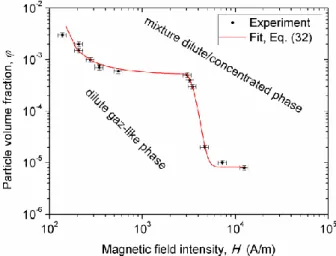
'( )H obtained at relatively long elapsed times (when the particle aggregation seemed to stop) is shown in double logarithmic scale in Fig. 6. The region below this curve corresponds to the dilute gas-like suspension phase of the suspension. The region above and on the right from this curve corresponds to a mixture between the dilute and the concentrated liquid-like or solid-like phases. The technique described in Sec. III does not allow determination with confidence of the second coexistence curve
''( )H . The shape of the'( )H
curve has some similarities with the shape of the corresponding coexistence curve of the phase diagram calculated by Hynninen and Dijkstra42 for dipolar hard spheres. A step in the middle of the binodal curve could stand for transition between entropically driven73 to magnetically driven phase transition, as inferred from our previous study57. In our case, this curve was fitted by the following empirical formula, valid in the concentration range6 3
8 10 ' 3 10 and in the range of the magnetic field intensities 150H 12500 A/m:
2 2 1 1 2 1 1 ( ) , 150 3030 A/m; '( ) , 3030 12500 A/m, 1 a H h a H H H h H H e (32)
where the magnetic field intensity H is in A/m and the fitting parameters take the following values: a15.05 10 4, a22.90 10 A m 3 -1 , h1133 A/m, h23330 A/m, 18.259 10 6 , 27.072 10 4. The fitting curve [Eq. (32)] is shown in Fig. 6 by a continuous line.
Fig. 6. Experimental -H phase diagram of the nanoparticle suspension in the presence of a uniform magnetic field. Only one of the coexistence curves, '( )H , is available in experiments. Another coexistence curve ''(H) is unavailable and not shown here. The error bars correspond to the sum of the standard deviation on three independent
It is important to notice that the measured values of the threshold magnetic field correspond to unexpectedly low values of the magnetic field parameter [Eq. (10)] and of the dipolar coupling parameter p / 4 (both ranged between 10-2 and 10). The phase separation in magnetic colloids is usually expected at >1 and >1 and the reason for the phase separation at <1 and <1 very likely comes from relatively high polydispersity of magnetic particles, as discussed in details in Sec. IV-E.
B. Microstructure
Snapshots of the suspension microstructure at different elapsed times are shown in Fig. 7 for the intensity of the applied magnetic field H0=4.0 kA/m. The three columns correspond to the
three studied initial particle volume fractions 0=110-3, 210-3 and 310-3. The first raw
corresponds to the initial moment of time t=0 at which the magnetic field was applied to initially homogeneous suspension in the direction horizontal with respect to the page.
Upon the field application, elongated drop-like aggregates aligned with the applied magnetic field appear and are already distinguishable at the elapsed time t=1min (second row in Fig. 7). This means that the initial nucleation stage is very short and unobservable in our optical microscopy experiments. The aggregate size increases progressively with time. At relatively short times, t<5 min, the growth of individual aggregates is observed, certainly thanks to adsorption of magnetic particles from the surrounding fluid. At longer times, t>5 min, neighboring aggregates start to coalesce because of their dipolar interactions, when their length is comparable to the average distance between them. Coalescence seems to accelerate the aggregate growth until t≈15 min. However, at t>15 min, the average aggregate length becomes much longer than the distance between them and the coalescence rate seems to decrease, at least at the considered field, H0=4 kA/m, likely because of repulsive dipolar interactions between
aggregates.
Because of insufficient optical resolution, it was impossible to retrieve exact aggregate shape. Qualitatively, the aggregate width progressively decreases when moving from the aggregate center to the tips, as in the case of ellipsoidal shape supposed in the model. Conical spikes have not been detected on aggregate tips, as opposed to the experiments of Promislow and Gast30 on drop-like aggregates of magnetorheological fluids and to our previous experiments on phase condensation around a magnetized micro-bead55,57. In fact, the characteristic period
1/ 30/( a )
D g
of patterns arising during convective instability on the interface between two miscible magnetic phases74 is about one micron for our experimental case (here a is the
difference between the aggregate and the surrounding medium densities). This length scale is comparable to the aggregate width, such that the aggregate tip is likely unable to develop numerous spikes.
As expected, at increasing initial particle volume fraction 0, the aggregate size increases
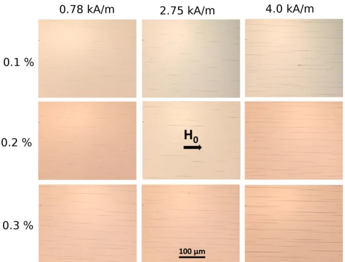
at a given elapsed time. The effect of the volume fraction and of the applied magnetic field on the aggregation state of the suspension can be better inspected on Fig. 8 where, all the snapshots are presented for the same elapsed time, equal to t=20 min but for three different values of 0
and H0. The suspension structure does not seem to change qualitatively with variations in 0 and
studied concentrations and fields. However, the aggregate length and thickness seem to increase considerably with increasing magnetic field and initial particle concentration and this effect will be inspected in detail in Sec. III-C.
Fig.7. Snapshots of the suspension microstructure at different elapsed times (different rows), for three initial particle concentrations 0 (different columns) and for the intensity of the applied magnetic field H0=4.0 kA/m
Fig. 8. Snapshots of the suspension microstructure at the fixed elapsed time equal to t=20 min and different intensity H0 of the applied magnetic field and different initial particle concentrations 0.
It is important to notice that the aggregates have a thickness of a few microns and the length of several hundreds of microns. Note that the aggregate thickness is governed by the interplay between magnetic and surface energy of the aggregates leading to Eq. (12) relating the aggregate volume to its shape. Their gravitational Péclet number is of the order of PeG102 and their sedimentation time (required for a horizontal aggregate to fall a distance equal to its width) is equal to a few seconds, so the aggregates are expected to sediment and reach the bottom of the cell during a few minutes. However, the images at different horizontal planes show that there are no aggregates near the bottom and the upper walls of the cell within boundary layers of a characteristic thickness of about 10 µm. This could be tentatively explained by magnetic levitation of aggregates dispersed in a dilute ferrofluid, when the lines of the magnetic field induced by the aggregate are “repelled” from non-magnetic walls and create an effective repulsion of the aggregate from the cell walls, by analogy with levitation of magnets in ferrofluids21.
C. Aggregate size
Our model was mostly focused on calculations of the elapsed time as function of the aggregate volume V. The three remaining geometrical parameters of the aggregates are easily related to the aggregate volume using Eqs. (11), (13). Thus, the aggregate aspect ratio ra is
directly given by Eq. (13b), while the aggregate length and width are given by the following expressions:
1/ 3 1/ 3 2 / 7 2 3/ 7 1/ 3 3 3 ˆ 1 ˆ 2 2 2 ln 7 a a Vr V V B , (33-a) 1/ 3 1/ 3 1/ 7 2 / 7 1/ 3 3 3 ˆ 1 ˆ 2 2 2 ln 7 a V b V V B r . (33-b)
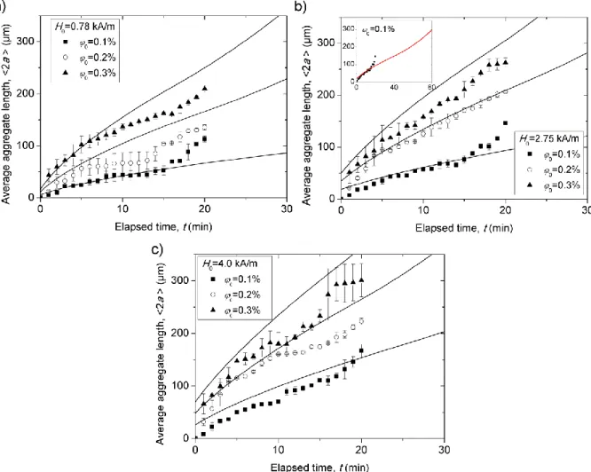
The most precise measured quantity describing the aggregate size is the average aggregate length 2a . Theoretical and experimental dependencies of the average aggregate length on elapsed time are presented in Figs. 9 a-c for three different values of the intensity H0 of
the applied magnetic field and for the three different initial particle volume fractions 0 of the
suspension. The most of experimental curves show an initial sublinear increase of the aggregate length with time, followed by a change in the slope at t≈10-15 min and by a stronger increase. Qualitatively, such a change of the slope corresponds to a transition between the aggregate growth and the aggregate coalescence regimes, as checked by tracking the snapshots [Fig. 7]. Since in experiments the aggregates had unequal lengths, the transition was progressive, i.e. occurred within finite lapses of times and aggregate volumes. Experiments also show that at the same elapsed times, the aggregate length is an increasing function of the magnetic field intensity H0 and of the initial particle volume fraction 0. This means that the aggregation process
accelerates with increasing H0 and 0. This was expected because an increasing magnetic field
enhances dipolar particle-particle, particle-aggregate and aggregate-aggregate interactions, while an increasing particle concentration reduces the time of approach of two particles and of two aggregates.
The theoretical dependence of the average aggregate length 2a on time is found in parametric form
2a f V1( ),t f V2( )
[Eqs. (33-a), (31)] and is presented by solid lines in Fig. 9. The aggregate magnetization M intervening into the timescale * of the coalescence stage was calculated in a linear approximation, M H0 with the aggregate magnetic susceptibility estimated using the Maxwell-Garnett mean field theory71:3 p ''/(1 p '') 3 ''/(1 '') 4.5
, where p 1 [cf. definition below Eq. (4)] and '' 0.6
- the internal volume fraction of aggregates [cf. Sec. II-A]. Two remaining unknown parameters, Vˆ0 and 0were found by fitting the experimental 2a versus t dependences by theoretical ones. Both these parameters have been found to strongly vary with the magnetic field intensity H0 and the initial particle volume fraction 0. The initial aggregate concentration 0 is
expected to be proportional to the concentration of the condensation centers in the suspension and is assumed to vary linearly with 0: 0 0. On the other hand, depending on the kinetics
of the early nucleation stage, the initial dimensionless volume Vˆ0 of aggregates could be an increasing function of both the magnetic field parameter and the initial particle volume fraction 0. We have supposed the empirical correlation
2
0 0
ˆ
V
for Vˆ0, which allows a reasonable agreement with experiments. Thus, all the nine experimental curves shown in Fig. 9 have beenfitted to the theory using the aforementioned expressions for 0, Vˆ0 and the single set of adjustable parameters and . The best fit was obtained at 3.3 10 4and 5.0 10 12.
Fig. 9. Experimental and theoretical dependences of the average aggregate length on the elapsed time for different initial particle concentrations 0 and different magnetic field intensities H0=0.78 kA/m (a); 2.75 kA/m (b); 4.0 kA/m
(c). Symbols stand for the experiments, solid lines – for the theory. The inset in (b) shows the same dependency for
0=0.1% in extended time scale. The experimental results were fitted by the theoretical dependences with the values of the adjustable parameters: 3.3 10 4and 5.0 10 12.
Our model seems to qualitatively reproduce the main experimental behaviors. First, one can distinguish a change of the behavior of the 2a versus t theoretical curves from sublinear to stronger than linear dependency. This change corresponds to the transition between two aggregation stages. The slope changes in a less abrupt manner than in experiments but rather continuously according to the proposed scenario of the transition based on equality of the aggregation rates [Sec. II-C]. The change of the slope can be better appreciated in inset of Fig.9b, where 2a versus t dependence is plotted for broader range of the elapsed times at H0=2.75 kA/m and 0=0.001. Second, the model captures the increasing dependence of the
aggregate length on the applied field H0. The magnetic field accelerates both stages of the phase
separation. During the aggregate growth stage, it decreases the correction factor K responsible for magnetophoretic particle flux and increases initial supersaturation 0 0 ' through a decrease of the equilibrium dilute phase concentration '(H0) according to Eq. (32) and Fig. 6.