Soz.- Präventivmed. 49 ( 2004) 224 – 226 0303-8408/04/030224–3
DOI 10.1007/s00038-004-3091-1 © Birkhäuser Verlag, Basel, 2004
Hints & Kinks in survey research
Estimating and approximating prevalence trends
Michael C. Costanza
Clinical Epidemiology Division, Department of Community Medicine, University Hospitals of Geneva
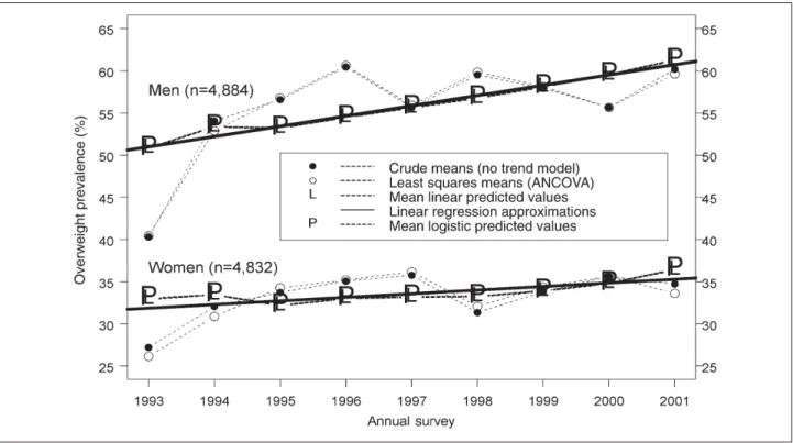
Figure 1 depicts gender-specific annual trends in overweight (body mass index (BMI) > 25 kg/m2) prevalence (%) for
nine independent, annual, cross-sectional samples of adult men and women (total n = 9 716) who were randomly se-lected within age strata during 1993–2001. Five different trend “curves” are shown. These ways of estimating or ap-proximating prevalence trends, and of assessing trend P-val-ues, are discussed in this Hints & Kinks.
1. Crude mean estimates (no trend model)
The dark circles are annual crude sample means of the over-weight “indicator” variable: Y = 100 for overover-weight
individ-uals, Y = 0 for non-overweight individuals. Thus, they are annual overweight sample prevalences, estimating Psurvey=
annual overweight population prevalences. (For propor-tions, code Y = 1 for overweight.)
Connecting crude means provides some idea of trend, but it is difficult to formalize this without a statistical model specif-ically designed to assess it.
2. ANCOVA “Least squares means” approximations Consider an analysis of covariance (ANCOVA) model for the population overweight prevalences by age (years, con-tinuous) and survey (9 groups (not concon-tinuous)),
Figure 1 Illustrations of the five approaches in Sections 1–5 for estimating or approximating annual trends in the prevalence of overweight (BMI > 25 kg/m2). The data are from nine independent, annual, cross-sectional samples of adult (35–74 years) men and women non-institutionalized residents of Geneva, Switzerland who were randomly selected within age strata from 1993 through 2001 (see Galobardes et al. 2003a; b). Each participant appeared in a single survey, and all analyses were gender-specific. Annual trend P-values: mean logistic predicted values estimates: men: P = 0.000027; women: P = 0.141; linear regression approximations: men: P = 0.000030; women: P = 0.137
225 Hinks & Kinks in survey research
Soz.- Präventivmed. 49 ( 2004) 224 – 226 © Birkhäuser Verlag, Basel, 2004
Costanza MC
Estimating and approximating prevalence trends
Page, survey= b0+ (b1 ¥age) + (b2 ¥survey), (1)
which is linear in age and survey for some unknown para-meters b0, b1, b2. Should neither age nor survey have effects
on being overweight (i. e., b1= b2= 0), then Page, survey= b0
(constant). It is an “additive” (assumes no (age ¥ survey) in-teraction effect) model.
Correspondingly, the open circles approximate
Psurvey= Page, survey– (b1 ¥age). (2)
Specifically, they are so-called “least squares means” (esti-mated “population marginal means”, Searle et al. 1980) ob-tained by analyzing the {Y, age, survey} data trio for each in-dividual using (e. g.) the “LSMEANS” option for survey (declared a “CLASS” (grouped) variable), in the SAS GLM (Generalized Linear Models) program (SAS Institute, Inc. 1999).
Connecting least squares means provides a further idea of (mean age-adjusted) annual trends (because age was in the model). However, this ANCOVA model was designed to as-sess any differences between annual prevalences, not trend, per se.
3. Mean linear predicted values approximations
If survey is continuous, the above ANCOVA model be-comes a (multiple) linear regression model. The (generic) b0,
b1, b2parameters (also approximations, say b0, b1, b2) are not
the same as before (e. g., b2is now a linear slope).
Neverthe-less, one can analyze the same (Y, age, survey) data with (e.g.) another GLM run (no “CLASS” declaration) to ob-tain approximations (“linear predicted values”) of Page, surevey
in (1),
L = b0+ (b1¥age) + (b2¥survey).
Then, an approximate Psurveyin (2) is the mean L over
indi-viduals in that survey.
Connecting mean linear predicted values (“L” points) pro-vides a “smoother” idea of trend than connecting crude or least squares means. (The “L” points are almost superim-posed on the “P” points, defined in Section 5.) However, al-though the linear regression model was designed to assess trend (because age and survey are continuous), this still does not constitute a formal test for trend.
4. Linear regression approximation
On the other hand, within the framework of the model in Section 3, the usual t- or F-test of H0 : b2= 0 (no survey slope)
does provide a formal assessment of (linear) trend. In the ex-ample, the annual overweight prevalences increased signifi-cantly in men (P = 0.00003), but not in women (P = 0.14).
In fact, however, these trend P-values refer to another (sim-pler) way of approximating (mean age-adjusted) Psurvey in
(2). Specifically, for each gender, the solid lines depict the single linear function of survey,
b0+ (b1¥mean age) + (b2¥survey),
i. e., the sample linear regression equation evaluated at the (overall) mean age.
5. Mean logistic regression predicted values estimates Although 0 ≤Page, survey≤100 since it is a percentage, it is
pos-sible to obtain a least squares mean, a mean linear predicted value, or even a point on the sample regression line outside that range because those approaches do not constrain the fi-nal approximated numerical values in any way. This is one reason why these three approaches were dubbed “approxi-mations” rather than estimates.
This difficulty is avoided by a logistic regression model and analysis. In lieu of modeling Page, survey directly, the
“logit” (or log odds) of Page, survey, which is the logarithm (log)
of {Page, survey/(100 – Page, survey)}, is modeled instead. The
cor-responding analogue of model (1) is:
log{Page, survey/(100 – Page, survey)} = b0+ (b1 ¥age) + (b2 ¥year).
(3) This model assumes the logit, not Page, yearitself, is linear in
age and survey (both continuous).
Once again, the individual (Y, age, survey) data are analyzed (e. g., with the SAS LOGISTIC program). In addition, cor-responding likelihood ratio tests (LRT) for trend can be ob-tained. In the example, the logistic LRT P-values were vir-tually the same as those reported in Section 4.
One can also estimate, for each individual in an annual sur-vey, the corresponding individual analogue of Psurveyin (2) by
back-transforming the estimated logit of Page, survey, (say)
LOGIT = {b0+ (b1¥age) + (b2 ¥survey)})
in two steps as follows: (i) exponentiate to eLOGIT, and (ii)
compute eLOGIT/(1 + eLOGIT). Then, to estimate the
corre-sponding (overall) analogue of Psurveyin (2), one can use the
mean eLOGIT/(1 + eLOGIT) over all individuals surveyed that
year (“P” points).
As mentioned above, in the figure the mean logistic pre-dicted values (“P”) were practically identical to the mean linear predicted values ( “L”). So, connecting the “P” points also provides a “smoother” idea of trends than connecting the crude or least squares means. However, neither the con-nected “P” nor “L” points is as smooth as the single regres-sion line approximation of Section 4.
Hinks & Kinks in survey research
Soz.- Präventivmed. 49 ( 2004) 224 – 226 © Birkhäuser Verlag, Basel, 2004
226 Costanza MC
Estimating and approximating prevalence trends
References
Galobardes B, Costanza MC, Bernstein MS, Delhumeau CH, Morabia, A (2003). Trends in risk factors for the major “lifestyle-related” diseases in Geneva, Switzerland, 1993–2000. Ann Epidemiol 13: 537–40.
Galobardes B, Costanza MC, Bernstein MS, Delhumeau CH, Morabi, A (2003). Trends in risk factors for lifestyle-related diseases by socioeconomic position in Geneva, Switzerland, 1993–2000: health inequalities persist. Am J Public Health 93: 1302–9.
Korn EL, Graubard BI (1999). Analysis of health surveys. New York: John Wiley & Sons.
MathSoft, Inc. (1999). S-PLUS 2000 user’s guide. Seattle, WA: Data Analysis Products Division.
SAS Institute, Inc. (1999). SAS OnlineDoc“,
VERSION EIGHT. Cary, NC: SAS.
Searle SR, Speed FM, Milliken GA (1980). Population marginal means in the linear model: an alternative to least squares means. Am Statist 34: 216-21.
Szklo M, Nieto FJ (2000). Epidemiology: beyond the basics. Gaithersgurg, MD: Aspen Publishers, Inc.
Address for correspondence
Michael C. Costanza, PhD Clinical Epidemiology Division Department of Community Medicine University Hospitals of Geneva (HUG) CH-1211 Geneva 14
Tel.: +41 22 372 95 52 Fax: +41 22 372 95 65
e-mail: [email protected]
Discussion and recommendations
Remember, prevalence estimates and trend P-values should be obtained by analyzing the individual-level data, not the aggregated (e. g.) least squares means data. Crude and least squares means were stressed in the first two approaches, but other types of adjusted means, or medians, etc., also could be used. SAS programs were cited, but others, e. g., in S-PLUS 2000 (MathSoft, Inc. 1999), used for Figure 1, could equally well be employed for the analyses.
In the moderately prevalent (25 % to 65 %) overweight ex-ample, there was little practical difference between the (technically more correct) mean logistic predicted values es-timates and the mean linear predicted values approxima-tions. Just as an observation, consistently similar degrees of concordance between these two approaches have occurred in our research on much less prevalent risk factors or out-comes (e. g., diabetes treatment prevalences from 0 % to 2 %). The even simpler, single straight line regression ap-proximations were also reasonably close to both the latter approaches for all prevalence magnitudes considered.
Further examples of the least squares means and linear re-gression approximations approaches can be found in Galo-bardes et al. (2003a; b), where quarterly trends in a variety of cardiovascular disease risk factors were assessed using these techniques.
The range of models covered here was curtailed and delib-erately simplified. Readers requiring more depth or more complex models for dealing with other important issues such as interaction effects, different methods of age-adjustment (e.g., direct standardization) or other covariate-adjustment, nonlinear trends, etc., are directed to more comprehensive references such as (e. g.) Szklo and Nieto (2000), or Korn and Graubard (1999).
Acknowledgements
The surveys were funded by the Swiss National Fund for Sci-entific Research (Grants No 31.326.91, 37986.93, 32-47219.96, 32-49847.96, 32-054097.98, 32-57104.99). The very constructive suggestions of two anonymous reviewers are greatly appreciated.