Smoking, Income and Subjective Well-Being: Evidence from Smoking Bans

HAL Id: halshs-00664269

https://halshs.archives-ouvertes.fr/halshs-00664269

Preprint submitted on 30 Jan 2012

HAL is a multi-disciplinary open access

archive for the deposit and dissemination of sci-entific research documents, whether they are pub-lished or not. The documents may come from teaching and research institutions in France or abroad, or from public or private research centers.

L’archive ouverte pluridisciplinaire HAL, est destinée au dépôt et à la diffusion de documents scientifiques de niveau recherche, publiés ou non, émanant des établissements d’enseignement et de recherche français ou étrangers, des laboratoires publics ou privés.

Smoking, Income and Subjective Well-Being: Evidence

from Smoking Bans

Abel Brodeur

To cite this version:

Abel Brodeur. Smoking, Income and Subjective Well-Being: Evidence from Smoking Bans. 2012. �halshs-00664269�

WORKING PAPER N° 2012 – 03

Smoking, Income and Subjective Well-Being:

Evidence from Smoking Bans

Abel Brodeur

JEL Codes: D62, H51, I18, I38

Keywords: Smoking policies, Subjective well-being, Social Interactions, Behavior

P

-

S

E

TÉL. : 33(0) 1 43 13 63 00 – FAX : 33 (0) 1 43 13 63 10

www.pse.ens.fr

CENTRE NATIONAL DE LA RECHERCHE SCIENTIFIQUE – ECOLE DES HAUTES ETUDES EN SCIENCES SOCIALES

1

S

moking, Income and Subjective Well-Being:

Evidence from Smoking Bans

Abel Brodeur Paris School of Economics

January, 2012

Abstract

This paper provides estimates of the effects of smoking policies on self-reported well-being using US county-level data. Because the bans were implemented at different times, it is possible to exploit these variations to identify the effect on a broad range of outcomes like self-reported well-being. The impact of smoking bans is estimated on those likely to be smokers relatively to others in order to take into account the effect on former, potential and current smokers. Our estimates suggest that the implementation of smoking bans make those who are predicted to be smokers more satisfied with their life. Within-family externalities and time-inconsistent family-utility maximization explain these findings. Additionally, there is evidence that the largest effect of smoking bans is for parents and married couples where the spouse is predicted to smoke.

Keywords: Smoking policies, subjective well-being, social interactions, behavior

JEL codes: D62, H51, I18, I38



PSE, 48 Boulevard Jourdan, 75014 Paris. E-mail: abel.brodeur@parisschoolofeconomics.eu. I would like to give thanks to my advisor Andrew Clark who helped me along the way. Financial support from the Fonds Québécois de la Recherche sur la Société et la Culture is gratefully acknowledged. Thanks to seminar participants at PSE. I am also grateful to Clément de Chaisemartin, Fabrice Etilé, Sarah Flèche, Pierre-Yves Geoffard, Mathias Lé, Karen Macours, Dimitris Alexandre Mavridis and Arthur Silve for valuable comments. I thank Chris Callahan, at DDB Needham, and Thomas A. Carr, at the American Lung Association, who answered my questions and provided data.

2

S

moking, Income and Subjective Well-Being:

Evidence from Smoking Bans

Abel Brodeur

Cigarette consumption and quality of life are to a large extent endogenous. Some smoke because they suffer from too much stress while others like sex for the cigarette afterward. It is therefore difficult to measure the impact of cigarettes on well-being. This being said, millions of premature deaths are due to smoking and about one third of adults are regularly exposed to second-hand tobacco smoke. Only 9% of countries mandate smoke-free bars and restaurants, and virtually no progress has been made in recent years. In 2009, the World Health Organization fostered governments to: “act decisively against the tobacco epidemic – the leading global cause of preventable death” (WHO, 2009). This recommendation is based on different studies that show the consequences of second-hand smoke. For instance, Laugesen and Woodward (2001) suggest that this cause of death lies between melanoma of the skin and road accidents in New Zealand. As pointed out by Fletcher Knebel: “It is now proved beyond doubt that smoking is one of the leading causes of statistics” (Reader’s Digest, December 1961).

This paper, part of continued work on smoking, seeks to illustrate certain links between smokers’ subjective well-being and smoking bans. The questions of whether tax changes, smoke-free workplaces and public bans may cause a decrease in smokers’ well-being are basic concerns for policy makers. This study is at the boundary of two lines of research. First, it deals with the literature on smoking policies and smoking behavior. The second line is the relationship between self-reported well-being and smoking. There is no consensus among researchers whether unhappiness may or not have an impact on smoking behavior. Veenhoven (2008) explains that happiness does not cure illness but could prevent it. Happy people tend to do more activities, and tend to be more reasonable with drinking and smoking. On the other hand, many people enjoy smoking and there is no clear evidence that happiness predicts starting or stopping smoking (Graham et al., 2004). A study by psychologists (Acaster et al. 2007) revealed that abstinent smokers

3 reported relatively lower levels of happiness than satiated smokers (recent smoked) when viewing pleasurable film clips. By contrast, sadness ratings weren’t affected by having smoked recently.

Our other line of research is more traditional to economists1. Using Australian data sets, Buddelmeyer and Wilkins (2005) exploit variation over time and States to gauge the effect of tougher smoking bans regulations on individuals’ smoking behavior. They find the intuitive result that the introduction of more severe smoking regulations increased quit probability and reduced starting probability (their estimates are not statistically significant though). Another point that should be mentioned is that the implementation of smoke-free public places may change smokers’ behavior. Anderson et

al. (2006) showed that smoke-free laws seem to stimulate adoption of smoke-free homes

which is a strategy associated with the success of these attempts. Within-family externalities thus need to be taken into account when examining the impact of smoking policies. Using British data (BHPS), Clark and Etilé (2006) found that there are intra-spousal correlations in smoking status in the raw data. They test whether these correlations come from the similarity of partners’ fixed traits (matching) or from decision-making over health investment. There is little evidence for spillovers in cigarette consumption between partners during marriage, but their estimates support the matching of partners’ preferences for smoking. It is thus essential that smoking policies target both partners in order to reduce household smoking.

Almost no attention has been paid to the question of whether smoking bans have a positive impact on individuals’ utility. One exception is the paper of Origo and Lucifora (2010) in which they estimated that European countries who introduced comprehensive smoking bans have been able to reduce the probability of exposure to smoke and the presence of respiratory problems for workers by 1.6 percent. These smoking bans produce also an adverse effect in increasing the probability of reporting irritability and anxiety at work.

1 _{A considerable literature exists on the effect of smoke-free workplaces on smoking behavior. See}

4 This research aims to contribute to the growing research on the determinants of life satisfaction by investigating how smokers’ subjective well-being has been affected by smoking policies. It was emphasized by Gruber and Mullainathan (2005, henceforth GM) that higher cigarette taxes could make predicted smokers less unhappy. People who stop smoking are obviously better off because of the health effects and the economic costs of smoking but these results go further in saying that smoking is an unwanted habit. Taxes provide a self-control device and allow smokers to do something they were not able to do, stop smoking. Next sections will come back on the reasons why stopping smoking is associated with higher subjective well-being. Hinks and Katsaros (2010) and more recently Odermatt and Stutzer (2011) also examined the relationship between well-being and smoking policies. Using respectively the BHPS and the Eurobarometer, their results reveal that smoking bans have no effect on life satisfaction of predicted smokers for the latter and a negative effect for smokers who reduced their daily consumption of cigarettes for the former. Additionally, Odermatt and Stutzer (2011) report that cigarette taxes affect positively nonsmokers which casts doubts on the external validity of the findings of GM. Our main objective is the examination of the impact of smoking bans on predicted smokers using a different identification strategy.

Counties have implemented smoking bans (bars or restaurants) at different times over the last 20 years in the US. This paper exploits these changes in policies to evaluate the effect of smoking bans on smokers’ subjective being. The self-reported well-being of people likely to smoke to people unlikely to smoke is compared after the implementation of smoking bans. The subjective well-being data come from the DDB Needham Life Style Survey (LSS) and the Behavioral Risk Factor Surveillance System (BRFSS). These surveys are cross-sectional and include a broad set of variables such as household income and smoking behavior. In addition, the chronological table of the

American Nonsmokers’ Rights Foundation gives the effective date of the first smoking

5 smokers stopped smoking2, it is not possible to check that the strongest impact is on smokers who stopped smoking as a result of the policies. Moreover, there is possibly an effect on potential smokers who could be discouraged by smoking policies. Using a measure of propensity to smoke allows us to estimate how smoking bans affect smokers who stopped smoking because of the ban, smokers who didn’t stop smoking, and finally potential smokers.

The central finding of this paper is that those who are predicted to be smokers report higher levels of well-being when a smoking ban is implemented. The estimates are large and robust to many specification checks. This is a surprising outcome for smokers since they do not, ex ante, favor the implementation of smoking bans. On the other hand, nonsmokers seem to be negatively affected by smoking bans which is as well a conundrum. Predicted smokers who are parents and married benefit the most from smoking bans. Lastly, I show that the results are driven by within-family externalities, since smoking bans have a positive effect through respondents’ spouse.

A number of theories are proposed to explain these results. The paper’s preferred explanation is time-inconsistent family utility maximization. Ex ante, smokers do not favor the implementation of smoke-free provision of smoking in restaurants or bars. However, these smoking policies make their family better off ex post which explains that they are more likely to agree that smoking should not be allowed in public places once they are affected by these bans.

The remainder of this article is structured as follows. The next section is devoted to the description of the data with detailed information on the questions used. Section 2 looks at some theories of addiction, and explores the socioeconomic determinants of voting behavior in the context of smoking bans using the LSS. The third introduces the methodology and the identification strategy. Section 4 presents estimates of the impact of

2 _{Cross-section data does not allow us to establish the evolution of well-being from current to ex-smokers.}

Unfortunately, virtually no progress can be made without consistent repeated cross-section or panel data in which there are repeated observations on individuals who quit smoking.

6 smoking bans on subjective well-being using the two data sets. The last two sections discuss the validity of the results and their interpretations.

Section I. Data and Subjective Well-Being

A. The Life Style Survey and the Behavioral Risk Factor Surveillance System

This paper examines how smokers’ well-being is affected by smoking policies. The methodology relies on using subjective data on life satisfaction. Our main data set is the DDB Needham Life Style Survey (LSS) which is a proprietary data archive that is freely available only for the period 1975-1998 on Robert Putnam’s Bowling Alone website3. The Life Style Survey started when the advertising agency DDB Needham commissioned the polling firm Market Facts to conduct an annual survey of Americans’ behaviors. This data set is repeated cross-section and includes different questions about subjective well-being. The time period covered with this survey is 1985-1998 (except 1990) since county-level data are not available for 1990 and only married people were interviewed over the period 1975-1984. County of residence is a key variable in this study since it is possible to assess the impact of county-level smoking policies on the residents of these counties. The timing and geographical variation provide an exogenous variation to estimate the effects of smoking bans on well-being. Moreover, the LSS is nationally representative in the United States and contains information on smoking behavior (except for the year 1998), gender, education level achieved, labor force status, marital status, household income, dwelling, and attendance at church or other place of worship. The LSS is an annual questionnaire which has a sample of around 3,500 American per annum. Our analysis is based on a total sample of 49,548 respondents.

Another data set is also used to investigate the impact of smoking bans. This allows us to check the robustness of our findings. Additionally, much more smoking bans have been implemented over the last decade which gives us more time variation. The time period covered is 2005-2010/10/01. The BRFSS is repeated cross section and

7 includes different questions about self-reported well-being4. It is nationally representative in the United States and it contains information on county of residence and smoking behavior5. This data set covers more than two thirds of the counties in the US and has a total sample of 1,671,273.

Numerous subjective well-being questions are tackled in these two surveys: feelings of confidence, pressure, future, direction of my life, family income satisfaction, and life satisfaction6. It is the last measure that is our main dependent variables. The following question is asked each year in the LSS: “I am very satisfied with the way things are going in my life these days” where respondents have 6 possible choices (6=definitely agree, 5=generally agree, 4=moderately agree, 3=moderately disagree, 2=generally disagree and 1=definitely disagree). Over the period 1985-1998 (except 1990), 16,24% of the respondents reported that they definitely agree that they are very satisfied with the way things are going in their life these days. On the other hand, 8,19% answered that they definitely disagree with this statement (see Appendix, Table 1). Similarly, the BRFSS includes a question on life satisfaction: “In general, how satisfied are you with your life?” where respondents have 4 choices (4=very satisfied, 3=satisfied, 2=dissatisfied and 1=very dissatisfied). Dummy variables (for instance, very satisfied and very dissatisfied) are used as our dependent variables in some specifications throughout this study.

These surveys also include questions on smoking behavior: “Do you now smoke cigarettes every day, some days, or not at all?” in the BRFSS and “How often you, yourself, use cigarettes at home or elsewhere?” in the LSS. Respondents who answer 52 or more times a year to the previous question are considered as daily smokers. In the

4 _{A third data set that could have been used here is the General Social Survey, but this was excluded for}

three reasons. The first reason is simply space consideration. Second, the public use version does not identify the State and the county of residence. I therefore purchased a restricted use version of the data (over the period 1993-2010). Lastly, data on smoking behavior is not available after 1994. Nonetheless, most of the findings are confirmed when turning to this data set (available upon request). Smoking bans have a positive effect on self-reported happiness of predicted smokers. For instance, the effect is very large and statistically significant when the sample is restricted to parents.

5 _{Over the period covered in this analysis, data on smoking is collected in 2005-2010 in the BRFSS. The}

BRFSS did not include a life satisfaction question before 2005.

6 _{One should note that studies pointed out that life satisfaction questions tend to elicit answers that are more}

reflective of life circumstances, and less reflective of ephemeral events, than do happiness questions (e.g. Deaton and Kahneman, 2010).

8 LSS, 21,77% of the respondents (weighted) report themselves as daily smokers (see Appendix, Table 1). This rate is going down over the waves which is consistent with prevalence rates of other surveys. Table 1 shows the mean and standard deviation of the variables in the LSS. Column 1 first presents these statistics for all the respondents, and then columns 2 and 3 do the same for respectively daily and non-daily smokers (occasional and nonsmokers). Over the whole sample, on average, daily smokers less agree with the statement that they are very satisfied with their life. 13,5% of daily smokers report that they definitely agree with the fact that they are very satisfied with the way things are going in their life these days against 16,9% for non-daily smokers.

B. Smoking Bans

Data on smoking policies in the United States come from the American

Nonsmokers’ Rights Foundation. The chronological table of the American Nonsmokers’ Rights Foundation indicates the effective date of smoke-free provision at the municipality

and county-level for bars and restaurants. It is then possible to know exactly which county has at least one municipality who implemented a smoking ban. In many counties, however, smoking in public places was prohibited by county-level laws. The first 100% smoke-free provision7 of smoking in a restaurant or a bar was the municipality of San Luis Obispo in 1990. Since the municipality of San Luis Obispo is located in the county of San Luis Obispo, all residents of this county are considered to be affected by the smoking ban. Using this methodology, respondents of 363 counties have been affected by smoking bans over the period 1990-2010/10. In addition, more than 30 States (Utah was the first in 1995) have implemented smoking bans. All the respondents in these States are thus affected by these smoking policies. Nowadays 75% of the U.S. population is covered by a smoking ban either for bars or restaurants.

Since our goal is to capture the impact of these smoking bans on smokers, pre-smoking ban periods are defined as the years/months/days before the law was effective.

7 _{Only counties with ordinances or laws that do not allow smoking in attached bars or separately ventilated}

9 A variable for whether the county of residence8 was affected by a complete interdiction of smoking in bars or restaurants is constructed. This indicator called “Smoking Ban” is then equal to one for all respondents living in the county that is affected by the smoking ban in each subsequent year/month/day, since the law is still valid. Date of interview is available in the BRFSS but not in the LSS. For the latter, post-smoking ban periods are defined as the years during and after the implementation of the bans.

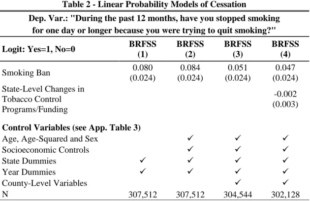
Table 2 reports the coefficients of the variable “Smoking Ban” from linear probability models of smoking cessation. I use the following question from the BRFSS as the dependent variable: “During the past 12 months, have you stopped smoking for one day or longer because you were trying to quit smoking?”. The period covered is 2005-2010 and the sample is restricted to smokers (daily and occasional). Statistically significant results suggest that when smokers are affected by smoking bans, they are more likely to quit smoking. Unsurprisingly, the coefficient is positive and significant at the 1% level (col. 1). Controlling for socioeconomic characteristics, county-level variables and state-level changes in tobacco control programs/funding does not affect this finding (from the American Lung Association: State of Tobacco Control). The probability they stopped smoking increases by two percentage points when exposed to a smoking ban. The sizes of the estimates are not large relative to the baseline levels of 58 percent of the sample who answered “Yes”. Interestingly, the effect of smoking bans is much larger when the sample is restricted to some demographic groups (i.e. parents, not shown for space consideration). Unfortunately, these estimates do not capture the effect on former and potential smokers. Moreover, some smokers could also decrease their cigarette consumption but still continue to smoke.

C. Subjective Well-Being

The literature on subjective well-being in economics has grown rapidly over the last decades (Kahneman and Krueger, 2006). Many surveys have reviewed the

8 _{In the United States, a county is a subdivision of a State. The average number of counties per State is 62}

10 relationship between income and subjective well-being (Clark et al., 2008; Di Tella and MacCulloch, 2006; Frey and Stutzer, 2002). While there is no clear conclusion whether more income brings more happiness, the social context and the reference group are among factors determining this relationship. Recent researches by economists have shown that the behavior of peer groups affects decisions of individuals. This means that well-being is influenced by decisions of peers. In the case of cigarettes, the decision to stop smoking is going to affect the behavior and the well-being of relatives. If my own disutility of smoking decreases with the prevalence of smoking of my peer groups, then spillover effects will occur. With the implementation of smoking bans, the prevalence among my relatives drops and my own disutility increases.

This research follows the proposition of Frey and Stutzer (2006) in using the economics of happiness as a methodological approach to evaluate whether a particular behavior (e.g. smoking) is sub-optimal and hence could reduce individuals’ well-being. Much research has pointed out that daily smokers report lower levels of well-being (Jürges, 2004; Shahab and West, 2009; Veenhoven, 2008). Unfortunately, these studies do not tackle the causality issue which is one of the weaknesses of this literature. Using longitudinal data (British Household Panel Survey), Moore (2009) showed that there is a robust relationship between change in daily cigarette consumption and well-being: a reduction of cigarette consumption improves self-reported happiness. Once again, this could mask reverse causality since smokers could feel better and then smoke less.

Section II. Smoking Bans and Addiction

Our initial intuition is that individuals who smoke are those who suffer the most from smoking bans in restaurants and bars. On the other hand, nonsmokers could benefit from these policies for a couple of reasons including the long term consequences of second-hand smoking9. Following the implication of a basic rational addiction model, smoking bans should decrease smokers’ well-being which explains why they are

9 _{A 2007 survey by Gallup indicates that about 40% of respondents (smoker or not) agree that smoking in}

11 relatively more resistant to these policies. Becker and Murphy (1988) explained that smoking policies create a dead-weight loss by changing consumers’ consumption choices. Even with addictive goods like cigarettes, taxes and smoking bans would cause a decrease in well-being for smokers. Individuals decide to smoke based on the long-run cost and immediate benefit of such a decision. A ban would thus decrease their direct pleasure by decreasing the number of places in which they are allowed to smoke.

The findings of GM are therefore quite surprising: predicted smokers report being less unhappy when cigarette taxes increase. They explain their findings with time inconsistency. In the model of Gruber and Koszegi (2001), smokers would be better off with excise taxes since this provides a self-control device. Individuals would like to stop smoking but they cannot because cigarettes are addictive. The same can be said with smoking ban since, in America, a majority of smokers want to quit. Gruber and Koszegi (2001) reported evidence that approximately eight out of ten smokers express a desire to quit. In this formulation, agents are patient about the future but impatient about the present. Smoking more in the short term increases pleasure, which explains why smoking policies would have positive effects on welfare.

Boyes and Marlow (1996) pointed out another issue related to the Coase Theorem10. Owners of restaurants/bars allocate airspace to the demanders (smokers and nonsmokers) in order to maximize expected profits. They argue that smoking bans, by reallocating the ownership of scarce resources (from the owners to the government), transfer income from smokers to nonsmokers. Nonsmokers receive an income transfer since they are not required to compensate smokers nor breathe smoke-filled air.

In 2002, a large telephone survey, conducted only on smokers (in Australia, Canada, United States and United Kingdom), reported that support for smoke-free environments is stronger when individuals have experienced bans (restaurants or bars). Gender and age are also good predicators of support: men and older smokers were in a

10 _{This theorem predicts that private markets internalize negative externalities when there are no}

12 greater proportion in favor of public smoking bans (Borland et al., 2006). Using data from a 1992 survey of 764 individuals in San Luis Obispo (CA), Boyes and Marlow (1996) found that the probability of supporting a ban in bars and restaurants is lower for smokers than for nonsmokers. Being an ex-smoker only influences negatively support for a ban in bars.

A question on smoking in public places in the LSS allows us to verify the findings of Boyes and Marlow (1996). Respondents are asked over the period 1985-1995 if: “Smoking should not be allowed in public places”. This is a 6-point scale question which goes from “Definitely Disagree” to “Definitely Agree”. The results of estimating regressions that relate being in favor of smoking bans in public places to a variety of socioeconomic determinants like being a smoker are presented in Table 3. State and year fixed effects completely control for any fixed differences between States and between years. Determinants of supporting or not smoking in public places include sex, age, marital status, household income, education, dwelling, attending church or other place of worship, children, working status and being a smoker. For all our equations in this paper, the personal sampling weights (the variable WEIGHT in the LSS) from each cycle are re-scaled to sum up to one for each year11. Moreover, the standard errors are corrected for autocorrelation by clustering at the county-level (Bertrand, Duflo and Mullainathan (2004)).

Column 1 first corroborates the finding of Boyes and Marlow (1996) that daily smokers are more resistant to the implementation of smoking bans. Being educated, living in a trailer, being a man, being married, attending church or other place of worship and working full-time increase significantly the probability to agree that smoking should not be allowed in public places (not shown). The latter determinant could be explained by the fact that smoke-free workplaces are not included in the question. The coefficients on age-squared show a clear U-shaped relationship between age and being in favor of

11 _{See Pfeffermann (1993) and Angrist and Pischke (2008) for a discussion on the role of sampling weights.}

Sampling weights are used in this study to have nationally representatives sample. The number of observations varies from wave to wave which explains our choice to re-scale equally each year. Also, our choice to include sampling weights has no impact on our analysis. Similar findings are obtained when sampling weights are not included.

13 smoking bans in public places. Additionally, it seems that there is not a monotonic relationship between the dependent variable and household income or having children.

The first column pointed out that daily smokers are not in favor of smoking bans. Column 2 looks at a different issue by investigating whether smokers who have been exposed to a smoking ban are in favor of these policies ex post. A dummy (“Smoking Ban”) indicating if the respondent’s county of residence has a smoking ban either in bars or in restaurants is included. Then, an interaction between “Smoking Ban” and “Daily Smoker” is added to capture the effect for smokers of being in a county with a smoking ban. The OLS shows a positive and large coefficient for the interaction, suggesting that daily smokers who are exposed to a smoking ban are less-opposed to these smoking policies.

These results are somewhat consistent with the model of Gruber and Koszegi (2001). Many surveys pointed out that smokers want to quit. However, smokers do not want to cease smoking in the present because they are impatient. Their long term objective is unreachable unless they are pushed to stop. After the implementation of smoking bans, they are more willing to say that bans should be allowed since it is a useful self-control device.

Section III. Smoking Bans and Well-Being: Empirical Strategy

This section tests empirically the hypothesis that smoking bans are important tools for increasing the well-being of predicted smokers: for former smokers, smoking bans helped them to realize their intentions to quit which are often not achieved; for current smokers, since cigarettes are addictive substances, any policies that reduce the frequencies of smoking might make them better off; and even for potential smokers, who could be discouraged to start to smoke. In order to do so, county-level smoking policies in the United States are used over the period 1985-2010.

14 Our methodology is the following: compare the subjective well-being of people likely to smoke to people unlikely to smoke after the implementation of smoking bans. Since much of the second-hand tobacco smoke effect on health occurs in the long-run, non-daily smokers are our control group. Many of the socioeconomic determinants in our data sets differ between daily and non-daily smokers (see Table 1). Daily smokers are, on average, less educated, younger, less likely to attend churches or place of worship, more likely to be unemployed, married, divorced, and to have children. These characteristics help us to predict if the respondent is a daily smoker. Regressions that relate smoking behavior to the following list of variables are estimated: age, age-squared, sex, interaction between age and sex, household income categories12, education categories, marital status, number of children, dwelling (only in the LSS), attend place of worship (only in the LSS), working status, and State dummies. Also, the log of the state-level changes in tobacco control programs/funding and the log of the state-level changes in excise taxes were used in some specifications (not shown) to predict smoking13.

Regressions are estimated for each year that has smoking behavior information14 in order to give to each respondent a predicted probability of smoking (PSMOKE). An example of this equation is shown in Appendix Table 3 for the year 1993 (2005 for the BRFSS). The pseudo R-squared is 0.14 for the LSS (0.10 for the BRFSS) and some variables like age, education, and attend place of worship are clearly important determinants of smoking. Our basic specification does not include an exclusion restriction in the equation that predicts smoking. Some alternative specifications (see Section V) will include such restrictions.

Our econometrics model is as follows:

12 _{Income is available only categorically in the LSS. I created a variable representing the log real family}

income per equivalent = 1 + 0.5 [other adults] + 0.3 kids. Using this measure or the 12 income categories does not affect the results of this paper.

13 _{The American Lung Association kindly provided the data over the period 2000-2010.} 14

Since there is no question on smoking behavior in 1998 in the LSS, the last year available (1997) is used to predict smoking for respondents of the wave 1998. Also, the methodology that is used to predict smoking does not affect the findings of this paper. Predicting PSMOKE with a regression for each year or with the first year in which there is a smoking ban or with all the years do not change the main estimates.

15 (1) SWBijt = α + βj + ηt + δSBjt + θPSMOKEijt + γSBjt*PSMOKEijt + ζXijt

where SWBijt is the outcome variable (for instance: life satisfaction) for respondent i in county j in year t, βj and ηt are State and year fixed effects, SBjt is an indicator for smoking bans (either for bars or restaurants) which is set to 0 if the county had not such a policy, PSMOKEijt is the predicted probability of smoking, and Xijt is a set of covariates that were used to predict smoking. In this setting, γ is the coefficient of interest.

One could worry that other time-varying factors correlated with the implementation of smoking bans would explain our results. This is why State-specific trends and county-level variables (Zjt) are added for some specifications:

(2) SWBijt = α + βj + ηt + δSBjt + θPSMOKEijt + γSBjt*PSMOKEijt + ζXijt + λZjt + tjt

I estimate OLS on a standardized variable (life satisfaction answers are standardized for all respondents within each wave to have a mean of zero and a standard deviation of one), but also alternative specifications like ordered probit models and linear probability models to explore whether the results are robust. As before, the personal sampling weights (WEIGHT) from each wave are re-scaled to sum up to one for each year. Standard errors are clustered at the county-level.

Section IV. Smoking Bans and Well-Being: Findings

A. Basic Results

Table 4 shows our basic findings of equation (1) using an OLS. While columns 1 and 2 look at the life satisfaction question described in Section III, the dependent variable of column 3 is: “I wish I could leave my present life and do something entirely different”. This is a 6-point scale question which goes from “Definitely Disagree” to “Definitely Agree”. This second question is highly correlated with the life satisfaction question (correlation coefficient of 0.42) and gives similar findings. The first row of Table 4

16 presents the effect of smoking bans on the whole sample. Then, the next row shows the effect of being a predicted smoker on self-reported well-being.

In the case of life satisfaction, smoking bans (either for bars or restaurants) have very small and positive effects on life satisfaction, but this is not statistically significant. Column 2 introduces two variables (smoking ban and the interaction between smoking ban and predicted smoking) which affect negatively the coefficient on smoking ban. Predicted smokers are reporting relatively lower levels of life satisfaction which is consistent with the literature (Jürges, 2004; Shahab and West, 2009; Veenhoven, 2008). Our variable of interest, SB*PSMOKE, is on the third row. The estimated coefficient is large and statistically significant. This means that smoking bans have a small and insignificant impact for the whole population, but have large and positive effects on predicted smokers’ life satisfaction. Our estimates suggest predicted smokers expose to a smoking ban saw an increase in self-reported well-being equivalent to 1/2 of a standard deviation (0.533/1).

These findings advocate that bans in bars and restaurants15 result in a welfare improvement for three types of individuals: former smokers, current smokers, and potential smokers16. An explanation could be that the positive effect on people who stopped smoking daily is offset by the decrease in well-being for those who are not smoking. If this is accurate, our estimates on smoking bans (first row) could be driven by two opposing forces. It might seem surprising that the effect of smoking bans is insignificant for the whole population. But, as shown by Adda and Cornaglia (2010),

15 _{Doing the same exercise with workplace smoking bans, using the LSS, gives different findings (available}

upon request). The impact of these bans on predicted smokers is close to zero and the estimates are not statistically significant.

16

An alternative specification would be to interact smoking ban with being a smoker. As explained previously, this is inappropriate because smoking bans may have an impact on many types of smokers. Using smokers and not predicted smokers would not capture the effect of the bans on people who stop smoking, potential smokers and smokers who are now smoking occasionally. One way to show this fact is to present estimations of an altered version of equation (1) where the variable “Predicted Smoking” is replaced by “Smoker”. Appendix Table 4 shows the results of this estimation. For the LSS, there is a positive (statistically significant at the 16% level) impact of smoking bans on smokers’ life satisfaction but the coefficient is much smaller than the one estimated on the interaction between predicted smokers and smoking bans. Column 2 shows similar findings using the BRFSS (relatively smaller but statistically significant at the 1% level). This means that much of the effect of smoking bans on smokers goes through smokers who decreased their cigarette consumption or stopped smoking.

17 smoking bans can intensify the exposure of nonsmokers to tobacco smoke by displacing smokers to private places. Moreover, smoking bans could encourage use of cigarettes among nonsmokers since smoking looks less harmful (Bernheim and Rangel, 2004). In order to verify the effect on nonsmokers, a dummy indicating if the respondent has a low propensity to smoke (below the 25th percentile) is generated. I then regress on the same covariates as before but the variable PSMOKE is replaced by the dummy low propensity to smoke. Estimating the model with low propensity to smoke gives a negative coefficient on the interaction SB*PSMOKE but it is small and insignificant (not shown for space consideration).

The positive outcome for smokers is quite surprising because, as shown in section II, this group does not favor the implementation of smoking bans. On the other hand, the absence of positive effects for nonsmokers is unexpected since the only reason why smoking bans may cause a welfare improvement, in the model of Becker and Murphy (1988), is externalities. A complication in interpreting the consequences of bans on nonsmokers’ well-being is the evolution of life satisfaction. It is possible that our measure is under-estimating the long-run benefits of these smoking policies.

Moreover, it is conceivable that people who smoke less than once a day (before or after the smoking bans) are negatively affected by smoking bans. If they were occasional smokers before the ban but weren’t able to stop to smoke, then one could possibly imagine that they are better or worse off. To verify this hypothesis, a predicted probability of smoking (PSMOKE) is re-estimated for each respondent by considering people who smoked at least once over the last year as smokers (in the previous analysis, only daily smokers were considered as smokers). Occasional smokers might be affected as well by smoking bans. If it is the case, including this group should give a positive effect of smoking bans on predicted smokers. Once again, smoking bans have large, positive, and statistically significant effects on predicted smokers (not shown). This means that both daily and occasional smokers benefit from smoking bans. Given that the smoking bans affect both types of smokers, our analysis focuses on these individuals for the remainder of this research.

18

B. Specification Checks

A further set of robustness checks (not shown) explore whether the findings are sensitive to the structure imposed by the OLS. Our choice to present OLS estimates is based upon the findings of Ai and Norton (2003) who pointed out that interpreting interaction terms in a nonlinear model is not straightforward. Nonetheless, using an Ordered Probit yields similar outcomes on predicted smokers.

The findings presented in this section are confirmed when turning to the BRFSS. Table 5 reports our basic findings of equation (1) using an OLS. The first row of Table 5 presents the effect of smoking bans on the whole sample. Then, the next row shows the effect of being a predicted smoker on life satisfaction. As was the case with the LSS, being a predicted smoker is negatively associated with life satisfaction. The interaction between SB*PSMOKE, is on the third row. The estimated coefficient is positive and statistically significant at the 4% level for the BRFSS17. Column 2 shows the same specification using another dependent variable, emotional support. This is a 5-point scale question which goes from “never” to “always” getting the social and emotional support you need. The effect of the smoking bans is positive and significant at the 1% level.

Another issue with our results could be that some omitted county variables might be correlated with smoking bans. Table 6 presents results of altered versions of equation (1) for the LSS (see Appendix Table 6 for the BRFSS). Column 1 interacts the county unemployment rate with “Predicted Smoking” to capture any business cycle effects that would affect differently smokers and nonsmokers. Column two includes interaction between State dummies and State-specific linear time trends to take into account any movement in smoking bans and well-being. The third column does include an interaction between time trends and the variable “Predicted Smoking” to allow for different trends in

17 _{In addition to the period covered, many explanations could be proposed to explain the difference in the}

size of the coefficient of interest between the two data sets. First of all, the variables used to predict smoking are different (see Appendix Table 3). Secondly, more smoking bans have been implemented during the period 2005-2010 which make us believe that the estimates are more precise with the BRFSS. Lastly, the sample size is proposed as an explanation.

19 self-reported life satisfaction. Column 4 includes an interaction of each State dummies with “Predicted Smoking” which allows the impact to vary across States.

All these interactions do not affect the finding that smoking bans increase the life satisfaction of predicted smokers. The inclusion of the interactions of State dummies and a time trend even increase the magnitude of the coefficient of interest for most of the specifications. Besides, adding an interaction between the time trend and the variable predicted smoking (occasional and daily smokers) lowers slightly the effects of smoking bans on predicted smokers. On the whole, the introduction of these controls does not affect the robustness of our findings.

Lastly, column 5 includes the following list of county-level variables: the median household income, smoking prevalence rates (only the BRFSS)18, an interaction between smoking prevalence rates and “Predicted Smoking”, unemployment rate, the percentage of high school graduates, the percentage of owner-occupied housing, urbanization and population density. These county-level characteristics were included in the equation that predicts if the respondent is a smoker. Including or not the county-level variables to predict smoking does not affect the findings of column 5. The coefficient of interest slightly decreases/increases in the LSS/BRFSS. Moreover, there is a positive relationship between smoking prevalence rate and life satisfaction (not shown). The coefficient of the interaction smoking prevalence rates and “Predicted Smoking” is very large (0.703 (std.: 0.123)) which means that smokers’ disutility of smoking decreases with the prevalence of smoking. Smoking bans decrease smoking prevalence and increase the disutility of smoking.

18 _{The BRFSS was used to estimate county adult smoking prevalence. Smokers were defined as adults who}

reported having smoked ≥100 cigarettes in their lifetime and now smoke every day or some days. Using this information, I test whether the effect of the bans is larger when the smoking prevalence is lower/higher at the county-level. Interestingly, the effect on life satisfaction is larger when the smoking prevalence is lower which is consistent with models of social interactions.

20 Section V. Discussion

Previous findings would suggest, a priori, that the time inconsistent model is well suited to explain why predicted smokers are better off with smoking bans. As pointed out by Gruber and Koszegi (2001), most smokers want to quit but are not able. This self-control problem is problematic because smokers are impatient about the present. They desire to smoke less in the future but are incapable of doing so in the short term. Because of this time inconsistency, any smoking policies that would help smokers to quit would increase their well-being. Also, our results show that smokers do not recognize, ex ante, that smoking bans could help them to improve their utility19. The positive impact of quitting on life satisfaction and the change in perception regarding smoking bans ex post could be interpreted as evidence that agents are not rational when it comes to addictive goods.

One way to understand the mechanisms that explain why predicted smokers are more satisfied with their lives when they are exposed to smoking bans is to evaluate the impact of smoking policies on different demographic groups. Jehiel and Lilico (2010) proposed a model in which the agent has limited foresight. They argued that young people have a limited foresight (short horizon) and stop smoking when they get older as a result of having better foresight. Smoking bans would thus affect differently young and old smokers. Estimating separately for young (less than 50 years old) and old respondents (more than 50 years old) the impact of smoking bans on life satisfaction confirms this intuition. There is a positive effect for both groups but it is significantly larger for young in both the BRFSS and the LSS (not shown).

In the framework of a rational addiction model, smoking bans could increase smokers’ well-being if there are externalities within the family. The question of whether within-interpersonal externalities may explain our findings can also be answered by looking separately at married and single respondents. If smoking bans make smokers’

19 _{O’Donoghue and Rabin (1999) propose an alternative model in which individuals do not recognize their}

self-control problems. Our findings do not corroborate their model since smokers want to quit but want to do it in a painless way.

21 family members more satisfied with their lives, then the impact should be larger on married people. This paper follows the two propositions of GM for investigating this issue. First, Table 7 separately estimates our baseline model for married and unmarried (divorced, single, separated and widowed) using the LSS (see Appendix Table 7 for the BRFSS). This is a useful way to check if some demographic groups are more or less affected by smoking policies. Columns 1 and 2 present the estimates of an OLS for unmarried and married people. There is some evidence that the impact of smoking bans is bigger, among predicted smokers, for married relatively to unmarried individuals. The coefficient is larger and only statistically significant for the interaction between predicted smoking and smoking ban when the sample is restricted to married people. When the sample is limited to unmarried people, the impact of smoking bans do seem to be positive but the standard deviation is quite large. This is a first piece of evidence that within-family externalities might be driven our findings.

Columns 3 and 4 separately estimate our model for parents and non-parents. If our effects are due to intra-family externalities, there are reasons to believe that the impact of smoking bans is greater for parents than for non-parents. If relatives are better off with less smoking, then smokers are more likely to stop smoking. This responsibility effect is found since the estimated coefficients on the interaction between smoking bans and predicted smoking are only statistically significant when the sample is restricted to parents. The estimated coefficients are both positive but the effect is much larger for parents.

The second proposition of GM in order to verify if there are externalities within the couple is to estimate spousal predicting smoking20. The LSS is well suited to do so since age, working status and education level of the spouse are available. I estimate spousal predicted smoking as a function of the covariates used previously for the respondent, but using the spouse’s age, working status and education level21

. These

20

The role of the spouse in determining satisfaction has been shown to be critical for obesity (Clark and Etilé, 2011).

21 _{Age, working status and education level of the respondent are not included in the spousal predicted}

22 variables are considered to determine the probability of smoking but are not determinants of well-being: these variables are exclusion restrictions and identify the model.

Our specification also follows Wooldridge (2002) who proposes to use the nonlinear fitted values as the instrument in the well-being equation (1). Firstly, the spousal predicted smoking equation is estimated with the exclusion restrictions described above. Then, the predicted variable “Spousal Predicted Smoking” is introduced as the only independent variable in a regression where the dependent variable is once again being a smoker. This gives us a second prediction of the spousal predicted smoking variable. Lastly, this second “Spousal Predicted Smoking” variable is used as previously in equation (1). Using this strategy or simply plugging in equation (1) the “Spousal Predicted Smoking” variable yields similar results.

Columns 5 and 6 show the estimated effect of equation (1) where the sample is restricted to married people. The first row presents, as before, the effect of the smoking bans on respondents’ life satisfaction. The fourth and the fifth rows show the predicted smoking of the spouse and the interaction between smoking bans and the latter variable. Column 5 does not include the variable PSMOKE and the interaction SB*PSMOKE. The effect of the smoking bans is identified through spouse’s predicted smoking. The interaction between spouse’s predicted smoking and smoking bans on the fifth row clearly shows large and positive effects on life satisfaction for married persons. The impact is statistically significant which suggests a role for spousal smoking in determining respondent’s life satisfaction. Column 6 simply adds the variable PSMOKE and the interaction SB*PSMOKE. Once again, married couples where the spouse is predicted to smoke are made better off by the smoking bans. But the inclusion of these two terms affect considerably the interaction “Smoking Ban*Predicted Smoking”. The coefficient becomes negative, very small and insignificant. This means that within-family externalities are present and appear to explain our main results.

predict if the spouse is smoking but they are not included in the well-being equation. The period is restricted to 1986-1998 (except 1990) for the LSS because the age of the respondent’s spouse is not available in 1985. The F-Stat for the first-stage varies from 45 to 90 depending of the year.

23 Section VI. Summary and Conclusion

This paper has attempted to provide an analysis of the consequences of smoking bans on the well-being of smokers. Our analysis of the LSS and the BRFSS data allows us to evaluate empirically the implications of different addiction models. Under the rational addiction model of Becker and Murphy (1988), smoking policies make time-consistent smokers worse off. A similar conclusion is found in the model of Boyes and Marlow (1996) where smoking bans, by reallocating the ownership of scarce resources (from the owners to the government), transfer income from smokers to nonsmokers. On the other hand, Gruber and Koszegi (2001) explain that smoking policies provide a self-control device for smokers. Since most of the smokers wish to quit, smoking bans do increase their well-being.

The empirical results show that life satisfaction increases for predicted smokers once a smoking ban, either for bars or restaurants, is implemented in their county. These findings are consistent with the model of Gruber and Koszegi (2001) in which smokers are time inconsistent. By forcing 100% smoke-free provision of smoking in restaurants or bars, the government allows individuals to do what they were unable to do, stop smoking. Another finding of this research is that smokers do not, ex ante, favor the implementation of smoking bans. It is only when they are affected by these policies that they do start to agree that smoking should not be allowed in public places.

The effects of smoking bans are not confined to daily smokers. Occasional smokers benefit as well from these bans. Due to a lack of information on the exact moment where respondents stopped smoking, it was not possible to address the short and long term consequences of stopping to smoke. Even though empirical evidence suggests that smoking bans increase life satisfaction of predicted smokers, it is of general interest to know the evolution of their well-being. Unfortunately, finding a US panel that includes self-reported well-being and smoking behavior over a long period may not be the easiest task.

24 Finally, the impacts of smoking bans are explained by within-family externalities. Positive effects of smoking bans are found for parents and married couples where the spouse is predicted to smoke. Time-inconsistent family-utility maximization gives a plausible explanation of these findings. If relatives are better off with less smoking, then smokers should stop smoking. Once again, a time-inconsistency model explains the fact that current smokers do not support smoking bans in the present even if their family would benefit from it.

25 Bibliography

Acaster S., L. Dawkins and J. H. Powell (2007). “The Effect of Smoking and Abstinence on Experience of Happiness and Sadness in Response to Positively Valenced, Negatively, Valenced, and Neutral Film Clips,” Addictive Behaviors, vol. 32, pages 425-431.

Adda J. and F. Cornaglia (2010). “The Effect of Taxes and Bans on Passive Smoking,”

American Economic Journal: Applied Economics, American Economic Association, vol.

2(1), pages 1-32, January.

Adda J. and F. Cornaglia (2006). “Taxes, Cigarette Consumption, and Smoking Intensity,” American Economic Review, American Economic Association, vol. 96(4), pages 1013-1028, September.

Ai, C. and E. Norton, (2003). “Interaction Terms in Logit and Probit Models,” Economics

Letters, Elsevier, vol. 80(1), pages 123-129, July.

Anderson, S., R. Borland, K.M. Cummings, G.T. Fong, A. Hyland, and H.H. Yong (2006). “Determinants and Consequences of Smoke-Free Homes: Findings from the International Tobacco Control (ITC) Four Country Survey,” Tobacco Control; 15(suppl. 3): iii 42-50.

Angrist, J. D. and J-S. Pischke. Mostly Harmless Econometrics: An Empiricist’s Companion. Princeton University Press, 2009.

Becker, G. S. and K. Murphy (1988). “A Theory of Rational Addiction,” Journal of

Political Economy, vol. 96, pages 675-700.

Bernheim, B. D. and A. Rangel (2004). “Addiction and Cue-Triggered Decision Processes,” American Economic Review, American Economic Association, vol. 94(5), pages 1558-1590, December.

26 Bertrand, M., E. Duflo and S. Mullainathan (2004). “How Much Should we Trust Differences-in-Differences Estimates,” The Quarterly Journal of Economics, MIT Press, vol. 119(1), pages 249-275, February.

Boyes, W. J. and M. L. Marlow (1996). “The Public Demand for Smoking Bans,” Public

Choice, Springer, vol. 88(1-2), pages 57-67, July.

Buddelmeyer H. and R. Wilkins (2005). “The Effects of Smoking Ban Regulations on Individual Smoking Rates,” IZA Discussion Papers 1737, Institute for the Study of Labor.

Clark, A., P. Frijters and M. Shields (2008). “Relative Income, Happiness, and Utility: An Explanation for the Easterlin Paradox and Other Puzzles,” Journal of Economic

Literature, American Economic Association, vol. 46(1), pages 95-144, March.

Clark, A. and F. Etilé (2011). “Happy House: Spousal Weight and Individual Well-Being,” Journal of Health Economics, Elsevier, vol. 30(5), pages 1124-1136, September. Clark, A. and F. Etilé (2006). “Don’t Give up on me Baby: Spousal Correlation in Smoking Behaviour,” Journal of Health Economics, Elsevier, vol. 25(5), pages 958-978, September.

Deaton, A. and D. Kahneman, 2010. “High Income Improves Evaluation of Life but not Emotional Well-Being,” Proceedings of the National Academy of Sciences, 5 pages.

Di Tella, R. and R. MacCulloch (2006). “Some Uses of Happiness Data in Economics,”

Journal of Economic Perspectives, American Economic Association, vol. 90(12), pages

27 Fichtenberg, C. and S. Glantz (2002). “Effect of Smoke-Free Workplaces on Smoking Behavior: Systematic Review,” British Medical Journal, vol. 325, 7 pages, July.

Frey, B. S. and A. Stutzer (2007). “What Happiness Research Can Tell Us About Self-Control Problems and Utility Misprediction,” Economics and Psychology. A Promising

New Cross-Disciplinary Field. Cambridge, MA and London, England: MIT Press,

169-195.

Frey, B. S. and A. Stutzer (2002). “What Can Economists Learn from Happiness Research?,” Journal of Economic Literature, American Economic Association, vol. 40(2), pages 402-435, June.

Graham, C., A. Eggers and S. Sukhatankar (2004). “Does Happiness Pay? An Exploration Based on Panel Data from Russia,” Journal of Economic Behavior and

Organization, vol. 55, pages 319-342.

Gruber, J. H. and B. Koszegi (2001). “Is Addiction "Rational"? Theory and Evidence,”

The Quarterly Journal of Economics, MIT Press, 116(4), pages 1261-1305.

Gruber, J. H. and S. Mullainathan (2005). “Do Cigarette Taxes Make Smokers Happier,”

The B.E. Journal of Economic Analysis & Policy, Berkeley Electronic Press, vol. 0(1).

Hinks, T. and A. Katsaros (2010). “Smoking Behaviour and Life Satisfaction: Evidence from the UK Smoking Ban,” Discussion Papers 1019, University of the West of England. Kahneman, D. and A. B. Krueger (2006). “Developments in the Measurement of Subjective Well-Being,” Journal of Economic Perspectives, Vol. 20(1), pages 3-24, Winter.

Jehiel, P. and A. Lilico (2010). “Smoking Today and Stopping Tomorrow: a Limited Foresight Perspective,” Cesifo Studies, 56(2), pages 141-164.

28 Jürges, H. (2004). “The Welfare Costs of Addiction,” Schmollers Jahrbuch, vol. 124(3), pages 327-353.

Laugesen, M. and A. Woodward (2001). “How Many Deaths are Caused by Second Hand Cigarette Smoke?,” Tobacco Control, 10, 383:388.

Moore, S. C. (2009). “The Nonpecuniary Effects of Smoking Cessation: Happier Smokers Smoke Less,” Applied Economics Letters, 16:4, pages 395-398.

O’Donoghue, T. and M. Rabin (1999). “Doing it Now or Later,” American Economic

Review, vol. 89(1), pages 103-124.

Odermatt, R. and A. Stutzer (2011). “Smoking Bans and Life Satisfaction in Europe,” Working Paper, University of Basel, First Draft – March 15, 2011.

Origo, F. and C. Lucifora, 2010. “Smoking Bans in European Workplaces,” CESifo DICE

Report, Ifo Institute for Economic Research at the University of Munich, vol. 8(3), pages

36-42, October.

Pfeffermann, D., 1993. “The Role of Sampling Weights when Modeling Survey Data,” International Statistical Review, International Statistical Institute, vol. 61(2), pages 317-337.

Shahab, L. and R. West (2009). “Do Ex-Smokers Report Feeling Happier Following Cessation? Evidence from a Cross-Sectional Survey,” Oxford University Press, Society for Research on Nicotine and Tobacco.

Veenhoven, R. (2008). “Healthy Happiness: Effect of Happiness on Physical Health and the Consequences for Preventive Health Care,” Journal of Happiness Studies, vol. 9, pages 449-464.

29 Wooldridge, Jeffrey M. 2002. Econometric Analysis of Cross Section and Panel Data. Cambridge (Mass.): MIT Press, 752 p.

World Health Organization, Report on the Global Tobacco Epidemic: Implementing Smoke-Free Environment, 136 pages, 2009.

30 Table 1 - Summary Statistics, Life Style Survey

All Daily Smoker?

Yes No Difference Reported Life Satisfaction

[1] Definitely Disagree [6] Definitely Agree

4.019 (1.469) 3.790 (1.518) 4.084 (1.446) -0.300 (0.017) Very Satisfied with the Way...

"Definitely Agree" 0.160 (0.367) 0.134 (0.340) 0.167 (0.373) -0.037 (0.004) Very Satisfied with the Way...

"Definitely Disagree" 0.081 (0.273) 0.108 (0.310) 0.073 (0.260) 0.033 (0.003) Male 0.452 (0.498) 0.482 (0.500) 0.441 (0.497) 0.039 (0.006) Age 46.18 (15.89) 43.53 (14.07) 46.76 (16.28) -3.33 (0.180) Elementary School 0.027 (0.163) 0.034 (0.181) 0.027 (0.161) 0.006 (0.002) Att. High School 0.070 (0.255) 0.115 (0.319) 0.059 (0.235) 0.055 (0.003) Grad. High School 0.353 (0.478) 0.425 (0.494) 0.336 (0.471) 0.088 (0.005) Att. Colleg 0.287 (0.453) 0.283 (0.450) 0.286 (0.452) 0.000 (0.005) Grad. College 0.133 (0.339) 0.079 (0.270) 0.147 (0.354) -0.067 (0.004) Post-Grad. Educ. 0.129 (0.335) 0.064 (0.245) 0.146 (0.353) -0.082 (0.004) Mobile HM 0.071 (0.257) 0.102 (0.303) 0.063 (0.242) 0.041 (0.003) 1-Family Detached 0.724 (0.447) 0.673 (0.469) 0.738 (0.440) -0.068 (0.005) 1-Family Attached to House 0.046 (0.209) 0.048 (0.213) 0.045 (0.206) 0.004 (0.002) Building for 2 Families 0.043 (0.203) 0.055 (0.228) 0.040 (0.197) 0.015 (0.002) Building for 3+ Families 0.113 (0.317) 0.119 (0.323) 0.112 (0.315) 0.008 (0.004) Never Att. Church 0.255 (0.436) 0.373 (0.484) 0.220 (0.414) 0.147 (0.005) Att. Church 1-4 a Year 0.156 (0.363) 0.207 (0.405) 0.143 (0.350) 0.060 (0.004) Att. Church 5-8 a Year 0.067 (0.251) 0.080 (0.271) 0.064 (0.244) 0.017 (0.003) Att. Church 9-11 a Year 0.047 (0.213) 0.050 (0.218) 0.046 (0.209) 0.005 (0.002) Att. Church 12-24 a Year 0.073 (0.260) 0.070 (0.255) 0.074 (0.261) -0.003 (0.003) Att. Church 25-51 a Year 0.144 (0.352) 0.103 (0.304) 0.157 (0.364) -0.052 (0.004) Att. Church 52+ a Year 0.257 (0.437) 0.118 (0.322) 0.296 (0.457) -0.175 (0.005) Married 0.723 (0.447) 0.699 (0.459) 0.734 (0.442) -0.033 (0.005) Divorced 0.083 (0.276) 0.116 (0.321) 0.072 (0.258) 0.043 (0.003) Single 0.106 (0.308) 0.103 (0.304) 0.108 (0.310) -0.004 (0.003) Separated 0.015 (0.121) 0.022 (0.148) 0.010 (0.101) 0.011 (0.001) Widowed 0.073 (0.260) 0.059 (0.236) 0.076 (0.265) -0.016 (0.003) No child 0.488 (0.500) 0.438 (0.496) 0.497 (0.500) -0.058 (0.006) One Child 0.201 (0.401) 0.217 (0.412) 0.199 (0.399) 0.020 (0.004) Two Children 0.196 (0.397) 0.215 (0.411) 0.191 (0.393) 0.021 (0.004) Three Children or More 0.115 (0.319) 0.131 (0.337) 0.113 (0.316) 0.018 (0.004) Full-Time Worker 0.489 (0.500) 0.523 (0.500) 0.478 (0.500) 0.040 (0.006)

31 Unemployed 0.027 (0.162) 0.042 (0.200) 0.023 (0.151) 0.020 (0.002) Self-Employment 0.087 (0.281) 0.087 (0.282) 0.087 (0.282) 0.001 (0.003) Part-Time Worker 0.090 (0.286) 0.080 (0.271) 0.092 (0.290) -0.012 (0.003) Retired 0.154 (0.361) 0.108 (0.311) 0.166 (0.372) -0.059 (0.004) Disabled or Student 0.032 (0.176) 0.043 (0.202) 0.028 (0.166) 0.016 (0.002) Full-Time Homemaker 0.122 (0.327) 0.118 (0.322) 0.126 (0.331) -0.007 (0.004) Unemployment Rate (County) 6.09 (2.33) 6.18 (2.30) 6.34 (2.27) 0.146 (0.026)

N 44,793 9,055 32,396

Note: Sample means are weighted using the variable WEIGHT and the personal sampling weights from each wave are re-scaled to sum up to one for each year. Standard errors are in parentheses. The period covered is 1985-1998, except the year 1990. Column 1 is full sample means while 2 and 3 restrict the sample to daily and non-daily smokers respectively.

Table 2 - Linear Probability Models of Cessation

Dep. Var.: "During the past 12 months, have you stopped smoking for one day or longer because you were trying to quit smoking?" Logit: Yes=1, No=0 BRFSS

(1) BRFSS (2) BRFSS (3) BRFSS (4) Smoking Ban 0.080 (0.024) 0.084 (0.024) 0.051 (0.024) 0.047 (0.024) State-Level Changes in Tobacco Control Programs/Funding -0.002 (0.003)

Control Variables (see App. Table 3)

Age, Age-Squared and Sex _   

Socioeconomic Controls     State Dummies     Year Dummies     County-Level Variables _{ }   N 307,512 307,512 304,544 302,128

Note: All estimates are weighted using the variable _finalwt and the personal sampling weights from each wave are re-scaled to sum up to one for each year. Robust standard errors are in parentheses, clustered by county. The period covered is 2005-2010 and the sample is restricted to smokers (daily and occasional). Replacing "State-Level Changes in Tobacco Control Programs/Funding" by "ln (1+State-Level Changes in Tobacco Control Programs/Funding)" has not impact on the variable "Smoking Ban".

32 Table 3 - Smoking Bans in Public Places, Life Style Survey

Dependent variable: "Smoking should not be allowed in public places: [1] Definitely Disagree to [6] Definitely Agree?"

Regression Coefficients OLS (z-scores) (1) OLS (z-scores) (2) Daily Smoker -1.556 (0.016) -1.558 (0.016) Smoking Ban 0.035 (0.068)

Smoking Ban*Daily Smoker 0.166 (0.096)

Control Variables (see Table 4)

Age, Age-Squared and Sex  

Socioeconomic Controls  

State Dummies  

Year Dummies  

N. 34,922 34,922

R² 0.3103 0.3103

Note: All estimates are weighted using the variable WEIGHT and the personal sampling weights from each wave are re-scaled to sum up to one for each year. Robust standard errors are in parentheses. The period covered is 1985-1995, except the year 1990.