An aerosol climatology for global models based on the tropospheric aerosol scheme in the Integrated Forecasting System of ECMWF

HAL Id: hal-02550728

https://hal.sorbonne-universite.fr/hal-02550728

Submitted on 22 Apr 2020

HAL is a multi-disciplinary open access

archive for the deposit and dissemination of

sci-entific research documents, whether they are

pub-lished or not. The documents may come from

teaching and research institutions in France or

abroad, or from public or private research centers.

L’archive ouverte pluridisciplinaire HAL, est

destinée au dépôt et à la diffusion de documents

scientifiques de niveau recherche, publiés ou non,

émanant des établissements d’enseignement et de

recherche français ou étrangers, des laboratoires

publics ou privés.

tropospheric aerosol scheme in the Integrated

Forecasting System of ECMWF

Alessio Bozzo, Angela Benedetti, Johannes Flemming, Zak Kipling, Samuel

Remy

To cite this version:

Alessio Bozzo, Angela Benedetti, Johannes Flemming, Zak Kipling, Samuel Remy. An aerosol

cli-matology for global models based on the tropospheric aerosol scheme in the Integrated Forecasting

System of ECMWF. Geoscientific Model Development, European Geosciences Union, 2020, 13 (3),

pp.1007-1034. �10.5194/gmd-13-1007-2020�. �hal-02550728�

https://doi.org/10.5194/gmd-13-1007-2020 © Author(s) 2020. This work is distributed under the Creative Commons Attribution 4.0 License.

An aerosol climatology for global models based on the tropospheric

aerosol scheme in the Integrated Forecasting System of ECMWF

1_{European Centre for Medium-Range Weather Forecasts, Reading, UK} 2_{Institute Pierre-Simon Laplace, Sorbonne Université/CNRS, Paris, France}

a_{now at: European Organisation for the Exploitation of Meteorological Satellites, Darmstadt, Germany}

Correspondence: Alessio Bozzo (alessio.bozzo@eumetsat.int) Received: 24 May 2019 – Discussion started: 1 July 2019

Revised: 17 January 2020 – Accepted: 29 January 2020 – Published: 10 March 2020

Abstract. An aerosol climatology to represent aerosols in the radiation schemes of global atmospheric models was recently developed. We derived the climatology from a reanalysis of atmospheric composition produced by the Copernicus Atmo-sphere Monitoring Service (CAMS). As an example of an application in a global atmospheric model, we discuss the technical aspects of the implementation in the European Cen-tre for Medium Range Weather Forecasts Integrated Fore-casting System (ECMWF-IFS) and the impact of the new climatology on the medium-range weather forecasts and 1-year simulations. The new aerosol climatology was derived by combining a set of model simulations with constrained meteorological conditions and an atmospheric composition reanalysis for the period 2003–2013 produced by the IFS. The aerosol fields of the reanalysis are constrained by assim-ilating the aerosol optical thickness (AOT) retrievals prod-uct by the Moderate Resolution Imaging Spectroradiometer (MODIS) instruments. In a further step, we used modelled aerosol fields to correct the aerosol speciation and the verti-cal profiles of the aerosol reanalysis fields. The new clima-tology provides the monthly-mean mass mixing ratio of five aerosol species constrained by assimilated MODIS AOT. Us-ing the new climatology in the ECMWF-IFS leads to changes in the direct aerosol radiative effect compared to the clima-tology previously implemented, which have a small but non-impact on the forecast skill of large-scale weather patterns in the medium-range. However, details of the regional dis-tribution of aerosol radiative forcing can have a large local impact. This is the case for the area of the Arabian Peninsula and the northern Indian Ocean. Here changes in the radiative

forcing of the mineral dust significantly improve the summer monsoon circulation.

1 Introduction

Aerosols have an important impact on the radiative budget of the Earth–atmosphere system. They participate in the atmo-spheric radiative transfer directly by scattering and absorb-ing electromagnetic radiation and indirectly by interactabsorb-ing with cloud microphysics (e.g. Haywood and Boucher, 2000; Bellouin et al., 2005). The uncertainty in the total radia-tive forcing by natural and anthropogenic aerosols remains large (Boucher et al., 2013), and most recent global climate models include more or less sophisticated prognostic aerosol schemes to explicitly take into account the direct radiative impact of aerosols on radiation and their interaction with cloud microphysics and other components of the Earth sys-tem (e.g. Bellouin et al., 2011; Donner et al., 2011; Stier et al., 2005). The impact of aerosols on the skill of numerical weather prediction (NWP) models is less clear (Baklanov et al., 2018; Mulcahy et al., 2014), and conclusions vary de-pending on the diagnostics used (Reale et al., 2011) and on the spatio-temporal scales analysed (e.g. Rémy et al., 2015). Global and regional NWP models often employ an approxi-mate treatment of aerosol radiative forcing based on a clima-tological description of their spatial distribution. This choice is mainly due to the fact that coupling an NWP to an atmo-spheric composition model with a significant number (usu-ally on the order of 10) of additional prognostic variables increases significantly the computational burden of the

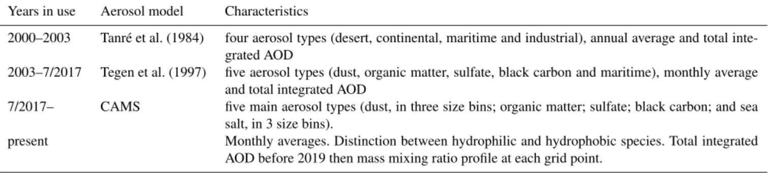
sys-Table 1. Evolution in the treatment of radiative effect of aerosols in the ECMWF-IFS forecast model. Years in use Aerosol model Characteristics

2000–2003 Tanré et al. (1984) four aerosol types (desert, continental, maritime and industrial), annual average and total inte-grated AOD

2003–7/2017 Tegen et al. (1997) five aerosol types (dust, organic matter, sulfate, black carbon and maritime), monthly average and total integrated AOD

7/2017– CAMS five main aerosol types (dust, in three size bins; organic matter; sulfate; black carbon; and sea salt, in 3 size bins).

present Monthly averages. Distinction between hydrophilic and hydrophobic species. Total integrated AOD before 2019 then mass mixing ratio profile at each grid point.

tem, but it might not translate directly into a clear improve-ment of the forecast skill (Morcrette et al., 2011; Mulcahy et al., 2014). Moreover, extra difficulties arise when assim-ilating real time observations to constrain the initialisation of the prognostic aerosol field because some species require an accurate prediction of their sources, as in the case of an-thropogenic and natural fires. A realistic representation of the mean climatological distribution of the most important aerosols can already improve the forecast skill both on a re-gional scale and globally (Rodwell and Jung, 2008).

With an increasing availability of large computer resources and the improvement of chemical transport models, an in-creasing number of studies explored the impact of includ-ing various levels of complexity in the representation of the aerosol radiative effect in NWP models (Baklanov et al., 2014). Mulcahy et al. (2014) concluded that including both direct and first indirect radiative effects of prognostic aerosols in a global NWP model results mainly in a reduc-tion in radiareduc-tion and temperature biases on the regional scale, with a limited impact on weather forecast skill. The represen-tation of the aerosol–cloud interaction remains uncertain, and this is so for its impact on NWP models.

The largest impact on weather the forecast skill of a prog-nostic aerosols scheme coupled to an NWP model is in case of events that are associated with large aerosol optical depths such as dust storms or wildfires. In these situations a realistic representation of the aerosol distribution differs significantly from the average climatology, and it can improve forecasts locally, especially close to the surface. Additionally, feed-backs linked to the direct aerosol radiative forcing can affect the production of the aerosol itself (Rémy et al., 2015). Sim-ilarly, Toll et al. (2015) and Zhang et al. (2016) showed that capturing the distribution of aerosols during extreme fires events has a significant impact on near-surface weather fore-casts for the affected areas.

In the operational configuration of the European Centre for Medium Range Weather Forecasts Integrated Forecast-ing System (ECMWF-IFS), the aerosol direct radiative effect has always been treated using climatological aerosol distri-butions, with no attempts at representing the interaction be-tween aerosols and cloud microphysics (Table 1). The IFS has employed since 2003 a monthly-mean climatology of

five main aerosol species based on one of the first multi-aerosol model simulations by Tegen et al. (1997) (TG97 hereinafter), and this substituted an earlier, simpler annual mean distribution based on Tanré et al. (1984) (Table 1). When the more-detailed TG97 climatology was introduced, it improved the model forecast skills mainly on a regional scale, but, thanks to teleconnection feedbacks, it also af-fected the large-scale mean flow (Rodwell and Jung, 2008). The tropical regions and in particular the monsoon areas of western Africa and India showed the largest sensitivity to the change in aerosol radiative forcing, resulting in improve-ments in the precipitation bias (Tompkins et al., 2005).

Prognostic aerosols were introduced in the IFS for the first time with the Global and regional Earth-system Monitor-ing usMonitor-ing Satellite and in-situ data (GEMS) project in 2005 (Hollingsworth et al., 2008) as part of the development of a real-time-operational assimilation and forecast capability for aerosols, greenhouse and reactive gases. The aerosol assim-ilation and forecast model (Morcrette et al., 2009; Benedetti et al., 2009) has been further refined in the subsequent Monitoring Atmospheric Composition and Climate (MACC) projects (Simmons, 2010), and it is now maintained and de-veloped within the Copernicus Atmosphere Monitoring Ser-vice (CAMS) as a suite of online integrated modules for aerosol and chemistry in the IFS (Flemming et al., 2015; Morcrette et al., 2009; Rémy et al., 2019). Morcrette et al. (2011) used an early version of the aerosol scheme in the IFS to explore the impact of coupled prognostic aerosols on the quality of the operational IFS forecasts. Both direct and indi-rect radiative effects were included, the latter impacting the number concentration of liquid cloud droplets according to Menon et al. (2002). They found that compared to the TG97 climatology, the changes in medium-range, large-scale fore-cast skill caused by having the prognostic aerosols interact-ing with radiation and cloud microphysics were small, al-though near-surface parameters showed local improvements. The inclusion of the full prognostic aerosol model had a pro-hibitive impact on the efficiency of the IFS, increasing the whole computational cost of the model by more than 50 %. However, no attempt at optimising the implementation was made.

A climatological description of aerosol distribution is still a viable option to capture the monthly-mean aerosol radiative effect for a NWP model (Toll et al., 2016). Improvements in aerosol climatologies are tied to improvement in chemical transport models and observations, and it can be represented as a 2- or 3D spatial distribution of aerosol mass or optical properties. A climatology can be built with a strong emphasis on surface observations using model fields to fill the gaps be-tween the sparse network of measurement sites (e.g. Kinne et al., 2013) or by merging model fields, satellite data and surface observations using empirical methods (e.g. Liu et al., 2005). A further option is to rely on a data assimilation sys-tem, which is the approach followed in this work.

The MACC reanalysis of reactive trace gases and aerosols (MACCRA, Inness et al., 2013) was the first multi-year atmospheric composition reanalysis effort developed with the MACC system, taking advantage of the 4D variational assimilation system (4D-Var) for atmospheric composition (Benedetti et al., 2009). Total aerosol optical thickness (AOT) was constrained by assimilating the AOT retrieved from the Moderate Resolution Imaging Spectroradiometer (MODIS) observations. CAMS is currently updating MAC-CRA with a new high-resolution atmospheric composition reanalysis (the CAMS reanalysis, CAMSRA), and as an in-terim product between MACCRA and CAMSRA, a new dataset (CAMS Interim reanalysis, CAMSiRA; Flemming et al., 2017) was produced. CAMSiRA shows a good agreement with the latest surface AOT observations, and combines the most recent advances in global aerosol modelling and satel-lite retrieval, so it represents an improvement with respect to the current TG97 climatology as well as MACCRA. It also provides a better framework to evaluate the impact of coupling the IFS prognostic aerosol model to the operational forecast system.

This document describes the development of a 3D monthly-mean climatology of five aerosol species based on CAMSiRA (Sect. 2). A comparison of the climatological val-ues against daily aerosol optical thickness observations will be discussed in Sect. 3. As an example of its application, in Sect. 4 we describe its implementation in the IFS, discussing the impact of the climatology on the mean model climate and on its forecast skills. The aerosol climatology is intended for public use, and it will be available through the CAMS data service.

2 CAMS aerosol climatology

The aerosol model implemented in the CAMS system is based on the model developed at the Laboratoire d’Optique Atmosphérique (LOA) and Laboratoire de Météorologie Dynamique (LMD) (Boucher et al., 2002; Reddy et al., 2005) with modifications by ECMWF during the GEMS and MACC projects. Details of the model can be found in

Mor-crette et al. (2009), Benedetti et al. (2009) and Rémy et al. (2019). Only a brief summary is given here.

Five types of tropospheric aerosols are considered: sea salt (SS), dust (DU), hydrophilic and hydrophobic organic matter (OM), black carbon (BC), and sulfate (SU) aerosols. Prog-nostic aerosols of natural origin, such as mineral dust and sea salt, are described using three size bins each (the size bins range is defined by the radius of the aerosol particle in mi-crometres, 0.03, 0.55, 0.9 and 20.0 for dust and 0.03, 0.5, 5.0 and 20.0 for sea salt) represented by three separate prognos-tic variables each. Hygroscopic effects are taken into account for sulfates, sea salt and organic matter. This means that the CAMS system computes a total of 11 prognostic variables. Emissions of dust depend on the surface wind (as measured at 10 m), soil moisture, the surface albedo in the UV-visible range and the fraction of snow-free land covered by veg-etation, with a correction to account for wind gusts (Mor-crette et al., 2008b; Rémy et al., 2019). The surface albedo in this case selects the area that can emit dust and weights the strength of the emission itself (Rémy et al., 2019). Emis-sions for sea salt depend on a source function based on Mon-ahan et al. (1986) and a representative at 80 % relative hu-midity (RH). Sources for the other aerosol types, which are linked to emissions from domestic, industrial, power genera-tion, transport and shipping activities, are taken from MAC-City annual- or monthly-mean climatologies (Granier et al., 2011). Emissions of OM, BC and SO2linked to fire

emis-sions are obtained using the Global Fire Assimilation Sys-tem (GFAS) based on MODIS satellite observations of fire radiative power, as described in Kaiser et al. (2011). The OM species include a contribution from organic carbon from bio-fuel, fossil fuel and biomass burning, with a small contri-bution of secondary organic aerosols from biogenic sources (based on terpene emissions). Sulfate aerosols are linked to SO2emissions, currently in a simple way parameterised in

terms of temperature and relative humidity to allow for the representation of the diurnal cycle. Further details about the parameterisation of the conversion rate between sulfur diox-ide and sulfate aerosols can be found in Rémy et al. (2019).

MODIS AOT data at 550 nm are routinely assimilated in a 4D-Var framework, extended to include aerosol total mixing ratio as an extra control variable using a variational bias cor-rection based on the operational setup for the assimilation of radiances, following Dee and Uppala (2008). A reader inter-ested in the details of its implementation in the IFS should re-fer to Benedetti et al. (2009) and Benedetti and Fisher (2007). As discussed in Flemming et al. (2017), the total AOT in CAMSiRA shows a good agreement with surface-based AERONET (Aerosol RObotic NETwork; Holben et al., 1998, 2001; https://aeronet.gsfc.nasa.gov, last access: 31 October 2019) observations. However, problems have been identified with the way the data assimilation distributes the contribu-tion of the various species to the total AOT, in particular introducing an unrealistically high sulfate burden over the oceans. We therefore derived the climatological distribution

of the 11 prognostic CAMS aerosol types using the CAMS Control Run (CR) setup alongside CAMSiRA and covering the period 2003–2013. This experiment uses the same me-teorological data and emissions as CAMSiRA but without data assimilation, hence leaving the aerosol species free to evolve. We then used the total AOT from CAMSiRA to con-strain this climatological AOT by scaling the monthly-mean distribution of the individual species to reproduce the total AOT computed in the reanalysis. Therefore, each monthly-mean AOT for the single species i at the grid point (x, y) is adjusted following the simple relation

AOTi,clim(x, y) =

AOTRA(x, y)

AOTCR(x, y)

×AOTi,CR(x, y), (1)

where AOTRAindicates the total AOT at 550 nm from the

re-analysis, and AOTCRis the total AOT from CR. Each species

is therefore scaled according to its contribution to the total AOT in a particular grid point.

The scaling computed from the AOT also applies to the mass mixing ratio, because consistent extinction coefficients are used between CR and CAMSiRA. The climatological scaled AOT is used only as diagnostic data in this work, while the actual aerosol climatology is computed in terms of a gridded, monthly spatial distribution of layer-integrated mass concentration (in kilograms per square metre) for each aerosol component over 60 vertical levels. We provide the mass concentration per layer because it will be directly pro-portional to the AOT given a mass extinction coefficient (in square metres per kilogram), since we believe this would be the primary use of such a climatology. A set of grid-ded monthly-mean pressure profiles is also provigrid-ded to al-low the conversion to mass mixing ratio (in kilograms per kilogram) and the interpolation to other vertical grids. The native horizontal grid of CAMSiRA is a reduced Gaussian grid with 80 grid points between the Equator and the poles (N80), equivalent to a linear grid resolution of approximately 1.125◦×1.125◦.

For the native CAMSiRA horizontal grid, the full 3D dis-tribution over 60 vertical levels has a size of ∼ 3 GB. The grid can be coarsened according to the desired resolution, and we found that a horizontal grid of 3◦×3◦with a total size of ∼500 MB was appropriate for the implementation in a rela-tively high-resolution global model such as the ECMWF-IFS with a spatial resolution equivalent to ∼ 9 km.

2.1 Spatial and vertical distribution of the mass mixing ratio

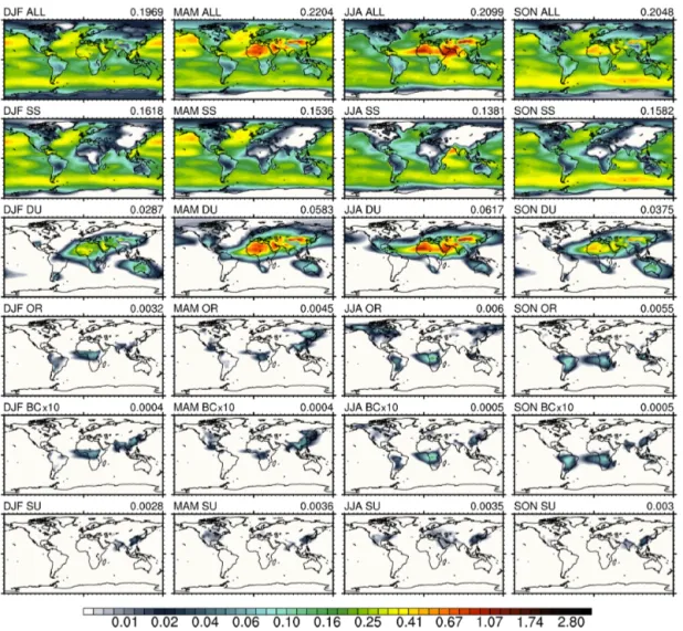
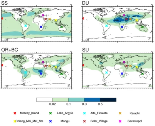
The spatial distribution of the integrated mass for each in-dividual type and for their sum shows marked regional and seasonal variations (Fig. 1). The largest contribution to the total global aerosol mass comes from mineral dust due to the large emissions over land, especially across the arid ar-eas of northern Africa and central East Asia in the Northern Hemisphere summer months. Sea salt is the most widespread

species, and it represents the second-largest contribution to the total global mass, with the highest concentrations found in the storm track areas of the Northern and Southern hemi-spheres. The organic matter and black carbon associated with the emissions from various anthropogenic and natural pro-cesses display a large seasonal variation and highly localised regional distribution. The sulfates are mostly distributed over the Northern Hemisphere, but the largest concentration is found close to the sources of anthropogenic emissions.

Each aerosol species exhibits a characteristic vertical dis-tribution with a distinct seasonal cycle, shown in Fig. 2 as zonal-average profiles. Sea salt is confined close to the sur-face, and it is strongly linked to the strength of the mid- and high-latitude winds, with a separate maximum around 15◦N associated with the Indian monsoon. Mineral dust is trans-ported vertically over the major desert areas of north Africa and Australia during the respective summer seasons, with a significant amount of mass up to 600 hPa in the Northern Hemisphere summer. The seasonal variation in the strength of the anthropogenic and natural organic emissions controls the amount and vertical extent of the organic and black car-bon species, with the main source located around the Equator and a June–July–August maximum in the Northern Hemi-sphere linked to the fire season in the high latitudes. Sulfate emissions, mostly from the industrialised areas peak, during the Northern Hemisphere summer with a maximum just be-low 700 hPa.

A small amount (< 1 × 10−3g m−2per layer) of aerosol mass is present in the upper tropospheric and lower strato-spheric layers, mostly at high latitudes. This process is likely to be overestimated in the CAMS model due in large part to the lack of any effective removal process for high-altitude aerosol (except for coarse dust and sea salt, which are sub-ject to sedimentation). This means that any excess of aerosol mass that the model places in the upper troposphere/lower stratosphere tends to have a long residence time and it affects the way the assimilation scheme vertically redistributes the total optical depth increments. This small amount of strato-spheric aerosol is therefore not to be considered as represen-tative of the contribution of stratospheric injection from large volcanic eruption. The AOT linked to stratospheric volcanic aerosols needs to be provided separately as the present cli-matology only represents the tropospheric aerosol species.

It is also possible to compute a characteristic climatolog-ical scale height for each species in order to describe the bulk of their vertical extent. This could be used to compute a simplified climatological vertical distribution for applica-tions that do not need a detailed description of the full 3D fields. Appendix A briefly discusses the details of the deriva-tion of such a parameter from the CR. The result is shown in Fig. A1, and, as seen in the zonal-mean profiles, it highlights regions where the aerosol species are transported away from the near-surface sources to higher levels.

Until recently the IFS used an implementation of the cli-matology from Tegen et al. (1997), which relied on an

ana-Figure 1. Seasonal vertically integrated aerosol mass (in grams per square metre) from the CAMS Interim reanalysis control run, scaled to conserve the total AOT of the assimilation run. The top row shows the total integrated mass for all aerosol types, and the other rows show the contribution from the single species for each season (see text for the abbreviations). Indicated in the top right of each map is the global average. Notice that values for the black carbon type (BC) have been multiplied by 10 for better visualisation, while the global average shows the unscaled value.

lytical function of type (p/p0)(H /ξ )to vertically redistribute

the aerosol optical depth. The function depends on the at-mospheric pressure p, the surface pressure p0, and the

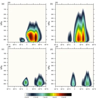
ra-tio between the scale height of the standard atmosphere H =8.4 km and a fixed global-mean scale height ξ for each aerosol component. A comparison of the vertical distribution of the aerosol mass in the CAMS climatology using this ap-proach to the real mean 3D distribution is shown in Fig. 3. Although in general the vertical profile is reproduced reason-ably well, the simplified analytical approach does not capture the elevated maximum between 850 and 700 hPa observed in the model data and stretches the upper boundary of the distri-bution too high. For species with non-negligible absorption in the solar spectrum, such as mineral dust and organic mat-ter, this means there is a vertical displacement in the solar heating rate profile, which impacts the temperature profile.

2.2 Spatial distribution of optical thickness

When looking at the total aerosol optical thickness (AOT), the contribution from the various aerosol types depends on the combination of their mass load and their extinction ef-ficiency. Since, in principle, any choice of optical proper-ties can be associated with the climatological distribution of aerosol mass mixing ratio, we will not attempt here a thorough discussion of possible refractive indices and micro-physical models to describe the radiative properties of each aerosol species. Instead, we will briefly focus on the dif-ference between the optical properties used for the CAMS aerosols in the implementation example discussed in the fol-lowing sections and those used for the aerosol climatology employed until recently in the IFS.

Until cycle 43r3 (2017), the radiative effect of aerosols in the ECMWF-IFS was computed using a monthly-mean

cli-Figure 2. Zonal-mean layer-integrated mass profiles (in grams per square metre), weighted by the total integrated mass at every grid point. Monthly average for January (left) and July (right). Notice that black carbon and sulfate values have been multiplied by 10 for better visualisation.

Figure 3. Zonal-mean layer-integrated mass profiles (in grams per square metre) average for July, weighted by the total integrated mass at every grid point for (a, b) mineral dust and (c, d) organic matter. Panels (a) and (c) show the zonal mean from CR fields, and (b) and (d) show the vertical profiles computed using an exponential function applied to the total integrated mass (see text). The scale height used for dust is 3 km, while for organic matter it is 2 km.

matology of total AOT based on the total mass load from TG97. The AOT vertical profile was computed analytically with an exponential function as described in Sect. 2.1 using a constant scale height ξ for each species, with ξ = 3000 for dust and ξ = 2000 for the other species. The climatology was coupled to the ECMWF radiation scheme (Morcrette et al., 2008a; Hogan and Bozzo, 2018) using optical properties de-rived from OPAC (Hess et al., 1998) and computed over a set of six coarse, broad band intervals with no dependence on the relative humidity from the model and a spatial resolution of 4◦×5◦.

To implement the radiative effect of the CAMSiRA aerosols in the IFS, we adopted the set of optical properties currently used in the IFS in order to diagnose the AOT from the CAMS aerosol forecasts. The details of the choices of size distributions and refractive indices for each species are discussed in more detail in Appendix B.

The largest differences in the optical properties used for the TG97 and CAMSiRA climatologies are found for the hydrophilic species organic matter and sulfates and for the hydrophobic mineral dust (Fig. A3). In the old climatology, sulfates and organic matter aerosols were combined as a sin-gle species, resulting in a generally larger absorption in the shortwave range when compared to the separate contribution from organic matter and sulfates in the CAMSiRA

climatol-ogy. The old optical properties for dust represented an aver-age of what can be expected across the three size bins used in the CAMS climatology but with significantly more absorp-tion across the solar spectrum between 2.0 and 0.4 µm and a much smaller total extinction at infrared wavelengths.

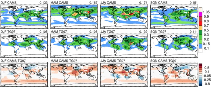
The total AOT distribution for CAMSiRA climatology is shown in comparison to the AOT from the old TG97 clima-tology in Fig. 4. The picture reflects the mass distribution seen in Fig. 1 with a strong seasonal variations both over land and over ocean. Compared to the AOT from the TG97 clima-tology, we notice a larger contribution from sea salt and a significantly different distribution over land. In particular the CAMS climatology has a larger AOT over the desert regions of northern Africa and central Asia as well as in the biomass burning areas of central Africa, North America, northern Asia and South America, the last of which also shows a dif-ferent seasonal cycle. The AOT is also larger over industri-alised areas in India and eastern Asia, while it is smaller over Europe due to changes in the industrial emissions over these regions, dominated mostly by sulfates.

We observe even larger differences in the absorption AOT (AAOT; Fig. 5), resulting from the combination of changes in the mass distribution and in the optical properties. The CAMS climatology captures with a finer resolution the emis-sion of black carbon and organic aerosols in central and east-ern Asia, while showing significantly less absorption over Europe. Also significantly different is the AAOT distribu-tion over Africa and the Middle East, where the TG97 clima-tology has a maximum in (June–July–August) JJA over the Horn of Africa, while the CAMS climatology has its maxi-mum over central Africa and the western Sahara.

3 Verification of the climatological aerosol distribution against surface observations

The accuracy of the CAMSiRA reanalysis and the CAMS aerosol model is discussed in Flemming et al. (2017), Inness et al. (2019) and Rémy et al. (2019) in terms of global and regional biases and correlation with surface observations in terms of AOT and particulate matter. Since the AOT com-puted from the climatology of the mass mixing ratio dis-cussed in this work is based on the same model, it has the same mean bias as the CAMS Interim reanalysis when eval-uated over a multi-year time interval. What we want to show here is how a monthly-mean climatology compares to a full prognostic aerosol scheme in terms of daily and intra-annual variability in aerosol distribution for a particular year.

To answer this question we used the observation from the AERONET network (Holben et al., 1998, 2001) for the year 2008 and compared them to the aerosol fields from the monthly-mean CAMS climatology and from the AOT for 2008 in the CAMS Interim reanalysis. We also included in the comparison the TG97 climatology that was used in the IFS until the model cycle CY43R3 (pre 2018). The

monthly-mean climatologies are linearly interpolated between the middle of each month.

The overall results over the whole globe and for five macro-areas are summarised in Table 2. The CAMSiRA cli-matology has a mean bias and correlation comparable to the corresponding reanalysis for the year 2008, with the lowest correlations observed over North America and Europe and the largest mean error over North America and South Amer-ica. Between the two climatologies CAMSiRA has in almost all of the regions higher correlations and lower mean bias than TG97.

The results from the global and regional scores can be un-derstood by looking in more detail at how a climatological description of the total AOT and the AAOT compares with the intra-annual variability observed in a particular year for a few locations (Fig. 7). We chose sites characterised by a dominant aerosol species and with different seasonal char-acteristics. The locations of the sites are shown in Fig. 6 to-gether with the contribution of the five main CAMS aerosol species.

For the comparison in terms of AAOT we use the L2.0, version 2, of the almucantar retrieval at each AERONET site (Dubovik et al., 2002; Holben et al., 2006). Given that the re-trieval products are available less frequently than direct AOT observations, we used an average over the 5 years of 2006– 2010 to increase the data coverage. The evaluation of the AAOT strongly depends on the choice of the optical proper-ties associated with the climatology, and therefore in the case discussed here it mostly reflects the single scattering albedo applied in the implementation of the climatology within the ECMWF-IFS (Appendix B). The absorption characteristics of the aerosol species are very sensitive to the refractive in-dex associated with each species and a thorough discussion of the quality of different sets of optical properties is beyond the main scope of this work.

Over Midway Island in the Pacific Ocean, the AOT is dominated by sea salt, with some contribution from sulfate aerosols, and both climatologies have comparable total AOT. Since the optical properties implemented for the CAMS cli-matology depend on the local relative humidity, here and for the other sites as well the daily AOT computed from the CAMS monthly-mean mixing ratio distribution inherits the synoptic variability in the humidity field. The compari-son of the AAOT against AERONET is not shown because the aerosols dominating this site have a very low absorption at visible wavelengths, yet we can see that the implemen-tation of the TG97 climatology likely also has too high of a mean absorption in areas that should not be subjected to large amounts of absorbing species.

Chiang Mai in northern Thailand represents a site with a seasonal influence from organic emission and industrial pol-lution in SE Asia. The seasonality in both AOT and AAOT is not captured in the TG97 climatology, while the CAMS climatology, although it clearly underestimates the peaks of AOT for the year in question, does reproduce the period with

Figure 4. Seasonal total extinction aerosol optical thickness at 550 nm. CAMS Interim reanalysis control run, scaled to conserve the as-similated AOT (top row) and the TG97 climatology (middle row). The bottom row shows the difference between the CAMS and the TG97 climatology.

Figure 5. As Fig. 4 but for absorption optical thickness.

a large aerosol amount between February and May. On av-erage the strength of the absorption is underestimated at the peak aerosol load.

In the Indian subcontinent both climatologies reproduce the seasonal variation in the AOT that is linked to the mon-soon circulation and the anthropogenic emissions. Both cli-matologies tend to underestimate the total AOT in northern India and Pakistan, with the CAMS climatology having an overall lower bias. As an example, at the Karachi site, influ-enced by dust and anthropogenic emissions, the two tologies have comparable total AOT, but the CAMS clima-tology shows a slightly larger AOT maximum between June and August. The AAOT curve shows much larger differences than AOT between the two climatologies, with too much ab-sorption for the TG97 climatology when compared against

the AERONET retrieval for most of the year. Both climatolo-gies seem to underestimate the absorption during the winter month, despite a relatively low AOT bias.

Mongu, Zambia, shows a peak in AOT between August and October that is linked to the seasonal biomass burning. The AOT from CAMSiRA with fully prognostic aerosols does a good job representing the daily variability linked to the organic species emissions, while the climatologies are able to represent the increase in mean AOT from July– August to October but obviously miss the variability linked to the single events. The underestimation of the AOT results in a slightly underestimated AAOT near the August–October peak, but it gives a good representation of the average ab-sorption conditions at the site.

Figure 6. Locations of the AERONET sites used in the analysis. The shading shows the annual mean AOT of the five CAMS aerosol species sea salt (SS), mineral dust (DU), organic matter (OR), black carbon (BC) and sulfates (SU).

Other areas show a very different representation of the seasonal cycle in AOT between the two climatologies, es-pecially over South America and Australia. For example at the Lake Argyle station, under the influence of mineral dust from the Australian interior and organic matter to the north, the CAMS climatology does a good job in capturing the min-imum AOT over the Southern Hemisphere winter months, while TG97 appears out of phase, perhaps due to the now-outdated emission inventories used in those earlier aerosol transport experiments. Not many data are available for the AAOT comparison at this site, though the few close to the peak period September–November suggest an underestima-tion in the total absorpunderestima-tion by both climatologies.

Again in the Southern Hemisphere, the station of Alta Flo-resta in South America shows a strong seasonal peak during the biomass burning season August–November. Although the CAMS climatology does capture this peak fairly accurately, it nevertheless overestimates it both in terms of total AOT and especially AAOT. The fact that AAOT has a large pos-itive bias is partially due to the overestimation in the AOT and possibly partially due to too large of an absorption as-sociated with the organic and black carbon species. This is related to some of the problems with the representation of biomass burning events in the CAMS model, as discussed in the Sect. 4.3.

Dominated by desert dust, Solar Village in Saudi Arabia shows a very variable AOT time series, reflecting the nature

of large dust plumes measured in the region. The CAMS cli-matology has a larger AOT than TG97 with a seasonal cy-cle capturing the larger dust activity over the April–August period. The AAOT in the CAMS climatology slightly over-estimates the average conditions retrieved by AERONET but does significantly better than the TG97 climatology, which greatly overestimates the absorption between May and Au-gust. This is an important difference, which can have a large impact on local atmospheric circulation, as discussed later in Sect. 4.4.

A final example representative of central and eastern Eu-rope where industrial aerosols dominate, the observations at Sevastopol on the Crimean Peninsula reveal a systematic bias in the TG97 climatology with an overestimation in both the AOT and the AAOT for the whole year. This bias is likely linked to the industrial emissions used in TG97 for Europe that are based on the Global Emissions Initiative (GEIA) database relative to the year 1985 (Benkovitz et al., 1996) and not representative of the emissions in the period 2003–2013 together with absorption characteristics that are too high, as-sociated with the industrial species.

4 The CAMS aerosol climatology in a global NWP model: implementation in the ECMWF-IFS

As an example of the use of the CAMS aerosol climatology in a complex global atmospheric model, we briefly discuss its

Table 2. Comparison between model and observation AOT for the year 2008 at AERONET sites. Model values are from the prognostic AOT from the CAMS Interim reanalysis (CAMSiRA 2008) and two climatological fields from TG97 and from the current work (CAMSiRA CLIM). The columns report the mean error and the correlation coefficient for five macro areas and globally for all sites. The size of the sample used to compute these statistics is reported in brackets in the observations (OBS) column.

OBS 2008 CAMSiRA 2008 Tegen et al. (1997) CAMSiRA CLIM Mean err. Corr. Mean err. Corr. Mean err. Corr. N. America 0.1341 (1425) 0.032 0.6678 0.037 0.369 0.040 0.4907 S. America 0.1603 (370) −0.006 0.8356 0.047 0.316 0.040 0.814 Europe 0.176 (1112) 0.009 0.6992 0.135 0.4187 0.015 0.4954 Africa 0.2689 (566) 0.009 0.7926 0.004 0.5373 0.005 0.7395 SE Asia 0.4329 (780) −0.056 0.6786 −0.142 0.4165 −0.07 0.6462 Global 0.215 (4259) 0.004 0.77 0.025 0.439 0.009 0.725

Figure 7. Comparison of daily mean total AOT at 500 nm for the year 2008 computed from the climatology presented in this work (red line), from the TG97 climatology (green line) and from the CAMS Interim reanalysis prognostic fields (grey line) at eight AERONET sites. The AERONET L2.0 daily mean observations are shown as blue dots. Please notice the different y axis for each plot.

implementation in the ECMWF global weather forecasting system (IFS).

We implemented in the IFS the full 3D CAMS climatol-ogy with the optical properties computed as described in Ap-pendix B, and we will discuss here the impacts of the new climatology compared to the IFS configuration using the old climatology based on TG97.

The implementation of the TG97 and CAMSiRA clima-tologies in the IFS radiation scheme differ in a number of ways. Both climatologies are represented in the radiation

scheme in terms of the three bulk radiative properties mass extinction coefficient (in square metres per kilogram), single scattering albedo and asymmetry parameter at each of the 30 spectral bands of the radiation scheme. For TG97, the opti-cal properties were computed based on the OPAC database (Hess et al., 1998) at a fixed value of relative humidity.

For the CAMSiRA climatology the optical properties are computed according to the description in Appendix B. For the hydrophilic species the optical properties are interpolated

Figure 8. Comparison of daily mean AAOT at 500 nm from the CAMS climatology (red line) and the TG97 climatology (green line), both as implemented in the ECMWF-IFS (see Appendix B for details) and AERONET data (blue dots). AERONET data are from L2.0, version 2, retrieval products (Holben et al., 2006; Dubovik et al., 2002) averaged over 5 years between 2006 and 2010. Please notice the different y axis for each plot.

to the relative humidity value provided by the IFS model at every grid point and vertical level.

Moreover, as already mentioned, CAMSiRA climatol-ogy is defined for each grid point and vertical level, while for TG97 an empirical vertical distribution is assumed (see Sect. 2.1)

The different impacts of the two climatologies in the IFS depend therefore on the combined effect of different aerosol spatial and vertical distributions and different radiative prop-erties.

4.1 Model experiments setup

In the following sections we will show the impact of the CAMS climatology on the IFS both in terms of changes in mean bias and in forecast skill, as measured by the correla-tion between modelled and observed large-scale atmospheric circulation.

All experiments are performed using the ECMWF model version 43R3 (operational from July 2017) with 137 verti-cal levels and prescribed sea surface temperature. We found that the results do not depend on the horizontal resolution of the model as long as it is high enough to represent well the subcontinental atmospheric circulations. This is because, as we will see in the following, the climatological aerosol ra-diative effect acts on broad areas, with largest impact on the bulk features of regional circulations. Therefore we adopted

for these experiments a horizontal cubic-octahedral grid at an equivalent resolution of 0.2◦ _{for efficiency. The CAMSiRA}

climatology was implemented with a horizontal resolution of 3◦×3◦, and a native vertical grid of 60 levels. The fields are interpolated online to the horizontal grid used in the radia-tion scheme (Hogan and Bozzo, 2018). This resoluradia-tion al-lows minimal impact on the model I/O while still being able to resolve the regional AOT features. Only the direct radia-tive effect of aerosol is taken into account in the IFS, with no attempt at representing indirect effects on the cloud droplet concentration and effective size.

We assess the model changes using two types of experi-ments; changes in mean radiative fluxes are assessed using a small ensemble of four 1-year runs over the period 2001– 2004 in which the IFS is left running unconstrained for a full year. We will refer to these experiments as “climate runs”.

The impact of changes in the aerosol climatology on the forecast skill is measured with a set of 10 d forecasts sepa-rated by 24 h over the periods May–August and December– February 2016, run twice, once with the new CAMSiRA cli-matology and once the older TG79 clicli-matology. Each fore-cast is initialised from the operational ECMWF analysis at 00:00 UTC and verified against the operational analysis. We will call these experiments “forecast runs”.

4.2 Impact on radiative fluxes

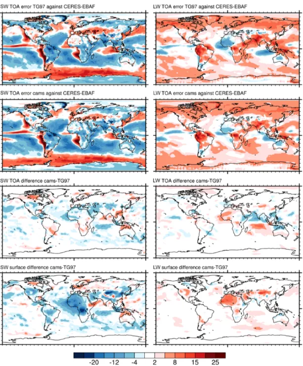
The change from the TG97 to the CAMSiRA climatology affects radiative fluxes in the long wave (LW) and shortwave (SW) both via direct interaction between aerosol and radia-tion and indirectly via changes in the cloud distriburadia-tion due to diabatic forcing on temperature. Using the climate runs we find that at the surface the net SW flux decreases in places by up to 20–30 W m−2in the larger AOT in the areas of large organic species emissions and over the deserts (Fig. 9, bot-tom). Although the large amount of sea salt aerosols over the oceans also contributes to a reduction of the surface net clear-sky SW radiation (by about 2–4 W m−2), this is less signif-icant given the larger contribution of cloud cover in those regions.

At the top of the atmosphere (TOA), the CAMS climatol-ogy increases the clear-sky reflected SW radiation globally with respect to TG97 by about 1–2 W m−2(not shown), but the effect on global all-sky fluxes is small, and the largest impacts are confined to small areas affected by large dust plumes transported from the Sahara desert over the Atlantic Ocean. Changes observed over the Indian Ocean and south East Asia (see Fig. 9, third row) depend mainly on local changes in the cloud distribution associated with aerosol-induced differences in regional atmospheric circulation. This aspect will be discussed in Sect. 4.4.

The impact on the LW fluxes is small, but it is significant in the regions with the largest mineral dust AOT, especially in the Northern Hemisphere summer months. The implemen-tation of the CAMS climatology with the optical properties described in the Appendix B brings to our tests an increase in downwelling LW radiation at the surface, which reaches more than 10 W m−2over the western Sahara and Saudi Ara-bia. This in part offsets the reduction in incoming SW radi-ation at surface in those areas, which is of the order of 10– 15 W m−2. At the TOA, significant differences in LW fluxes between the two climatologies are found only where clear-sky dominates. Over the deserts, high-level dust layers re-duce the upward emission to space, and the effect is stronger for the CAMS climatology, which has a larger amount of dust mass over the deserts.

Most of the bias in TOA fluxes computed from the IFS operational cycle 43R3 against the top of atmo-sphere fluxes provided by the CERES-EBAF project (Clouds and the Earth’s Radiant Energy System Energy Bal-anced and Filled; https://ceres.larc.nasa.gov/products.php? product=EBAF-TOA, last access: 31 October 2019) are due to errors in cloud cover and cloud amount (e.g. Ahlgrimm et al., 2018), and aerosols only play a small role (first two rows in Fig. 9). Therefore the modification in the aerosol dis-tribution brings only small local improvements. In particu-lar the change in the dust distribution over the western Sa-hara and central east Atlantic brings some local reduction in both LW and SW TOA flux bias by increasing by about 5– 10 W m−2the reflected SW radiation and slightly decreasing

by about 5 W m−2the outgoing LW radiation. Some further small changes in TOA fluxes are observed over the Indian Ocean, but this time they are not related to changes in the clear-sky radiation. Instead, a slight reduction in the cloud cover on the western coast of India indirectly improves the TOA fluxes by reducing the reflected SW radiation and at the same time increasing the outgoing LW radiation. This change in the total cloud cover in the area is related to changes in the aerosol radiative forcing, which modifies the summer mon-soon circulation, as discussed in Sect. 4.4.

4.3 Impact on forecast errors and skill

Using the forecast runs we can measure to what extent changes in the direct aerosol radiative effect affect mea-sures of forecast skill scores. The direct impact of a new aerosol climatology is to alter the radiative heating rate pro-files and the surface energy budget. The former dominates the change in forecasts errors, and it affects the mid- to lower-tropospheric temperatures. The latter mostly impacts the sur-face temperature. Although the change in AOT is spatially highly inhomogeneous and locally large, this does not ap-pear to be enough to impact the variability in the large-scale circulation.

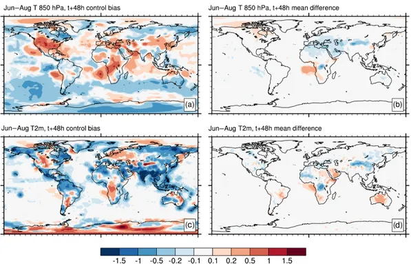
Two main regions show the largest impact on the lower-tropospheric temperature, and these are dominated by dust and organic/black carbon aerosols. Because of the combina-tion of the difference in total AOT and in optical properties, for the same AOT the CAMSiRA climatology reduces the absorption of SW radiation in dust-affected regions with re-spect to TG97. This induces a widespread decrease in tem-perature of about 0.1 K below 700 hPa after 48 h (Fig. 10), growing to more than 0.2 K at day 5. In the ECMWF model this helps in reducing by about one-third the positive tem-perature bias observed in the Mediterranean region and the Middle East. The effect is larger in the summer months due to the stronger mean solar radiation and the larger dust AOT. Another significant temperature change is observed below 850 hPa over the Gulf of Guinea and central Africa where the relatively large amount of biomass burning aerosol in the CAMSiRA climatology significantly absorbs SW radi-ation. In this case the ECMWF model already suffers from a positive temperature bias in the region, and the extra heating provided by the new aerosol AOT further increases the pre-existing bias. The radiative impact of the organic and black carbon species generally have a small but positive impact on the upper-air temperature biases over northern Canada in the summer months, although in these areas the seasonal vari-ability in the forest fires is naturally impossible to capture in a climatological distribution. Single events can be very signif-icant, and they need prognostic treatment to accurately take into account their impact on local weather parameters (Toll et al., 2015).

Surface temperatures are affected by the change in aerosol climatology only locally over central and northern Africa

Figure 9. Changes in multi-annual mean (2001–2004) net radiative fluxes (in watts per square metre) at the top of atmosphere (TOA) and surface for the shortwave (left column) and long wave (right column) in the IFS. The top two rows show the errors in the TOA fluxes when using TG97 and CAMS climatologies compared to CERES-EBAF observations. The last two rows show the change in the TOA and surface fluxes between the experiment using the CAMS climatology and the experiment using the TG97 climatology. Values above (below) 4(−4) W m−2indicate systematic features larger than the natural variability in the field.

and parts of Asia (Fig. 10), where changes in the AOT be-tween the two climatologies are the largest (see Fig. 4). In the biomass burning regions of central Africa, the decrease in surface SW radiation causes a decrease in the surface tem-perature, which helps in reducing the pre-existing positive bias. In northern Africa and Middle East the change in dust AOT is significant in the summer months, with surface cool-ing over the western Sahara and localised surface warmcool-ing

over Saudi Arabia where the significant increase in welling LW compensates for the smaller decrease in down-welling SW. Other significant temperature changes are found in Australia, where the reduction in dust AOT in the CAM-SiRA climatology causes surface warming and in the Tak-lamakan Desert in China, where the large dust AOT causes surface cooling.

Figure 10. Temperature at 850 hPa (in kelvin; a, b) and 2 m (in kelvin; c, d) for forecast time t + 48 h averaged during the 2-month period July–August 2016. Panels (a) and (c) show the error of the operational model, and (b) and (d) show the difference between a forecast experiment with CAMS climatology and the operational model using TG97. Model errors are computed against operational analysis.

The variability and forecast skill of large-scale extratropi-cal weather patterns are not significantly affected by these re-gional changes in temperature. Measures of the forecast skill, such as the anomaly correlation of mid-tropospheric geopo-tential, show virtually no impact (not shown), corroborating similar results of Morcrette et al. (2011).

Measurable impacts on hemispheric scores are found only for the temperature RMSE in the lower troposphere during NH summer (Fig. 11), due to the aforementioned changes in SW absorption by mineral dust and organic species. In particular, the temperature RMSE generally improves in the Northern Hemisphere by about 1 % in summer thanks to less SW absorption over the deserts, which reduces the persis-tent warm bias affecting the IFS in the Northern Hemisphere summer between the surface and 700 hPa.

In the tropics and partly in the Southern Hemisphere we found an increase by ∼ 1 %–0.5 % in the 850 hPa tempera-ture RMSE relative to the RMSE using TG97. This is dom-inated by the localised increase in forecast errors over the Gulf of Guinea (local increase in the RMSE by up to 20 %), which in turn affects the forecast skills over the tropical belt. The scarce availability of continuous observations in this area makes it difficult to have a good estimate of the real aerosol radiative effect, but the impact on the forecast runs suggests a bias in the CAMSiRA aerosols over the Gulf of Guinea given the significant departure from the temperature profile of the operational analysis. Independent estimates of AAOT for central Africa (e.g. Bond et al., 2013) seem in-deed to suggest a large overestimation in the CAMS model in

the summer months over central Africa. We identify as likely contributors to this bias (i) possible incorrect vertical distri-bution of all aerosols (including absorbing types) in the fore-cast model, driven in part by an incorrect weight of the con-tribution by convective transport and scavenging; (ii) a ten-dency for the assimilation to assign far too much relative im-portance to black carbon in the tropics compared to the other species; (iii) errors in the emission for organic and black carbon aerosols; and (iv) too large of an absorption in the optical properties associated with the organic and black car-bon species. These problems are currently being addressed, and improvements have been incorporated in the most recent CAMS reanalysis (Inness et al., 2019).

This analysis shows that although the impacts of a change in the aerosol climatology are small in terms of large-scale forecast skill scores, they can nevertheless be non-negligible, especially in areas where the model has pre-existing biases or where the model has particularly low errors and is therefore sensitive to small changes in the local radiation budget. On the other hand, impacts at the regional scale can be large. The most robust changes are found over the Indian Ocean during the summer monsoon season and are forced predom-inantly by a modified radiative forcing by the desert dust, which brings a reduction in the near-surface wind errors. Sec-tion 4.4 presents in more detail the feedbacks between the monsoon circulation and changes to the local AOT.

Figure 11. Normalised temperature RMSE difference at 1000 and 850 hPa for a set of forecast runs using the new CAMS climatology against the operational configuration. The experiments cover a summer season (2 May to 13 August 2016) and are verified against the operational analysis. Confidence range of 95 % with AR(2) inflation and Sidak correction for four independent tests (Geer, 2016). These experiments were done using a cubic-octahedral spectral truncation TCo399, but the main results are independent on the model resolution. Values < 0 mean that the forecasts with the CAMS climatology are better than those with the TG97 climatology.

4.4 Impacts on local circulations: the Indian summer monsoon

The area of the northern Indian Ocean during the summer monsoon season shows the largest feedback between changes in aerosol radiative forcing and regional-scale circulation. In this region the CAMS climatology has a different impact on radiative fluxes than the TG97 climatology as implemented in the IFS (Figs. 4 and 9). The largest change occurring with the CAMS climatology during summer is a decrease in total SW absorption over the Middle East and eastern Africa of ap-proximately 4–8 W m−2on average but exceeding 30 W m−2 over the Horn of Africa. This is due to both a change in the distribution of mineral dust mass in the region and to the higher dust reflectivity we adopted in the CAMS climatol-ogy.

Numerous studies have explored the sensitivity of the In-dian summer monsoon to aerosol radiative forcing from both anthropogenic and natural sources (Bollasina et al., 2011; Lau and Kim, 2006; Wang et al., 2009). By using a combi-nation of model and satellite data Vinoj et al. (2014) showed that the radiative effect of mineral dust over eastern Africa and the Arabian Peninsula affects the monsoon circulation over the Indian Ocean. The heating rate perturbation induced by the dust layer can modulate the strength of low-level west-erly zonal winds and moisture transport towards eastern and central India over timescales of weeks. The feedback was successively explored in detail by Jin et al. (2015) and Jin et al. (2016), showing the thermodynamic mechanism that links the dust radiative effect over the Iranian Plateau and precipi-tation variability on sub-seasonal timescales over western In-dia. This implies that a realistic representation of the aerosol radiative effect in the region can potentially have a

signifi-cant impact on the predictability of the monsoon circulation in medium-range and seasonal forecasts.

In the operational configuration pre-CY43R3 with uncou-pled sea-surface temperatures, the IFS has too strong of a near-surface westerly jet across the northern Indian ocean, from the eastern Africa to western India (Fig. 12a), which in turns causes conditions that are too wet over western In-dia during the summer months. This brings a positive pre-cipitation bias in the region of 1–2 mm d−1over land in the 3-month period June–August as compared to various esti-mates of surface precipitation (Table 3). The same circula-tion bias is also responsible for part of the errors in the top-of-atmosphere LW and SW fluxes (Fig. 9) observed in the climate runs, related to too much cloudiness over western In-dia.

The CAMS climatology brings changes in the mean winds and temperature below 700 hPa, and this reduces the forecast errors in the area both for the wind strength at all lead times (Fig. 12b) and also for the accumulated seasonal errors in precipitation amounts (Table 3). Further evidence of an im-proved mean model state also comes from the assimilation cycle. The increase in surface temperature and pressure over the Persian Gulf and Saudi Arabia helps to reduce the error of the forecast first guess with respect to the observations used in the assimilation step, indicating an improvement in the analysis fields because the model is closer to the obser-vations (not shown).

Near-surface westerly zonal wind strength decreases in the northern part of the Indian Ocean and increases to the south (Fig. 12b), implying a weakening and southward shift of the low-level jet. The changes grow larger at longer lead times due to the cumulative contribution of the modified radia-tive forcing acting from the very beginning of the forecast.

Table 3. Mean precipitation over western India (region boundaries: 25–6◦N, 67–77◦E) for JJA, estimated by different products and model bias for two forecast experiments for the period 2001 to 2004. Data are in millimetres per day.

GPCP v2.22 HOAPS3 v61,3 SSMI1,4 TRMM 3B435

OBS 5.5 5.1 2.5 6.4

TG97-OBS 2.1 0.2 4.1 1.3

CAMS-OBS 1.4 −0.3 3.8 0.5

1_{Values not defined on land grid points.}2_{Global Precipitation Climatology Project (Huffman et al.,}

2015).3_{Hamburg Ocean Atmosphere Parameters and Fluxes from Satellite Data (Andersson et al.,}

2010).4Special Sensor Microwave/Imager and Sounder (Wentz et al., 2012).5Tropical Rainfall Measuring Mission Multi-Satellite Precipitation Analysis (Huffman et al., 2007, 2010).

Figure 12. Near-surface (925 hPa) zonal wind for the period 1 May–21 August 2016 over the northern Indian Ocean for (a–c) forecast day 2 and (d–f) forecast day 10. Model bias using (a, d) TG97, (b, e) CAMS climatology and (c, f) the difference between forecasts using the CAMS climatology and TG97 climatology. Notice the different scale in the righthand side panels. Bold colours indicate areas significant at the 5 % level using a paired t test with AR(1) noise. The units are indicated above each figure.

These circulation changes are the result of a combination of large-scale and more localised perturbations to the tempera-ture gradients between the Indian Ocean and the land areas.

In the CAMS climatology, less SW radiation is ab-sorbed by the dust layer, causing a decrease in the lower-tropospheric temperature over the eastern Africa–Arabian Peninsula region (see Fig. 10), a key driver of the monsoon circulation over the Indian Ocean (Vinoj et al., 2014; Jin et al., 2016, 2015). Following this lower-tropospheric cooling, the geopotential height decreases over land above 500 hPa, inducing upper level convergence and localised descending motion, which partially balances the radiative cooling. This causes an increase in the surface pressure and geopotential height at low levels over the Middle East and Arabian Penin-sula, improving the model bias by up to 30 %–50 % (Fig. 13). The higher pressure below 800 hPa reduces the low-level

convergent flow over the continental areas, resulting in a weaker north-eastward circulation in the northern section of the Indian Ocean.

Moreover, although in the IFS, aerosol concentrations do not directly impact cloud microphysics, the changes in the local atmospheric circulation and the vertical distribution of heating rates can cause an indirect impact of aerosol on cloudiness. Over the Indian Ocean the weaker monsoon cir-culation implies a reduced average cloudiness, with a clear impact in the radiative fluxes at the top of atmosphere, as ob-served in Sect. 4.2.

We tested how much these effects depend on the absorp-tion properties of dust using the optical properties computed from different the refractive indices such as Dubovik et al. (2002), with less absorption at shorter wavelengths (see Ta-ble A3), and we found that very weakly absorbing dust

pro-Figure 13. As Fig. 12 but for the geopotential at 925 hPa (in metres squared per second squared).

duces an even stronger decrease in the monsoon circulation (not shown), confirming the previous findings (Vinoj et al., 2014). This sensitivity, together with the fact that in our ex-periments the sea surface temperature (SST) are prescribed and that we do not explicitly simulate the interaction between aerosol and cloud microphysics, indicates that the direct at-mospheric heating by the dust layer is the main factor behind the observed circulation changes.

5 Conclusions

This work documents a new monthly-mean climatology of aerosol distribution based on the Interim reanalysis from CAMS (CAMSiRA, Flemming et al., 2017) and its control run. The dataset represents a monthly-mean distribution of the mass mixing ratio of five aerosol species subdivided into 11 types over 60 vertical levels. The climatology is available at full native resolution for the 3D fields or at any coarser hor-izontal grid. The user can associate the radiative properties of choice with the aerosol distribution, and here we present re-sults that used the bulk properties for each species computed for the 30 radiative bands of the ECMWF radiative scheme (Hogan and Bozzo, 2018).

We tested the impact of the CAMS climatology on the ECMWF Integrated Forecasting System in comparison to the aerosol climatology operational until summer 2017, which was derived from Tegen et al. (1997).

Compared to AERONET observations over number of years, the CAMSiRA climatology captures fairly well the mean seasonal variation in the total AOT, while the

depen-dence of the optical properties on the relative humidity helps capturing at least part of the daily variability. We used the AAOT retrieved from AERONET sites to test the AAOT re-sulting from associating the optical properties used in the ra-diation scheme of the ECMWF-IFS with the present clima-tology. The comparison showed generally a good agreement, but it did also highlight the uncertainty in the definition of the single scattering albedo over various regions, in particu-lar when they are dominated by biomass burning events. We did not attempt a thorough discussion of the variety of re-fractive indices associated with the various species, and the user has the opportunity to experiment with different optical properties.

When implemented in the ECMWF-IFS, the new CAM-SiRA aerosol climatology affects the radiative fluxes and brings small improvements locally to biases both in the short-wave and in the long short-wave spectrum compared to satellite ob-servations. These changes in aerosol radiative forcing with respect to the ECMWF implementation of the Tegen et al. (1997) climatology are due to a different spatial distribution, different radiative properties and different representation of the size distribution of each aerosol species.

In the ECMWF-IFS, the change in the climatological representation of aerosol distribution has a limited impact on commonly used measures of hemispheric forecast skill scores, and it does not affect significantly the variability in the large-scale synoptic circulation, in agreement with re-cent studies (e.g. Morcrette et al., 2011; Mulcahy et al., 2014; Toll et al., 2016). Locally, temperature changes in the lower troposphere can be of a similar order of magnitude as the

pre-existing model biases and can therefore affect the model mean state.

Larger impacts are found in areas where there is a stronger link between clear-sky radiative perturbations and local cir-culation. In the ECMWF model, the Indian summer monsoon over the Indian Ocean shows a marked sensitivity to the min-eral dust radiative forcing over eastern Africa and Saudi Ara-bia. The magnitude of the absorption by mineral dust mod-ifies the mean temperature and geopotential over the Mid-dle East land areas and the Indian Ocean, which in turn af-fects the north-eastward branch of the Indian monsoon. In the ECMWF model this reduces by about 30 % the mean model bias in lower-tropospheric geopotential and zonal wind, also improving the representation of precipitation over the north-ern Indian Ocean and south-westnorth-ern India.

The CAMS prognostic aerosol model is in continuous de-velopment and future releases of this aerosol climatology will incorporate the latest improvements in aerosol mod-elling and data assimilation.

Appendix A

A1 Vertical scale height of the CAMS aerosol types We can derive an estimate of the scale height ξ for each aerosol type from the vertical distribution of the mass mixing ratio in the CR. Generally ξ depends on the aerosol spatial distribution and the season, and it can be found by calculat-ing at every grid point the height at which the normalised cumulative mass distribution reaches the value 1/e. The spa-tial distribution of ξ is shown in Fig. A1 for July and January for all aerosol types.

The scale height of mineral dust exhibits the largest spatial and seasonal variations because of the strong dependence of the dust emission and transport on the height of the bound-ary layer mixing over the deserts and the seasonal patterns of large-scale synoptic circulations. The dust species is the only one exhibiting a large seasonal cycle, with ξ ranging from ∼2 m in winter rising to ∼ 3 km in summer. For the other species, ξ can be approximated by a constant value through-out the year. Sea salt aerosols and black carbon are generally confined to the lower levels with ξ ∼ 1 km, while the organic matter extends higher with ξ ∼ 2 km. As sulfate is formed from SO2, which has sources from both anthropogenic

ac-tivities and from oceanic dimethyl sulfate, it occurs further over most of oceans and continents and tends to have a more homogeneous distribution with ξ ∼ 3 km (Fig. A1).

Table A1. Refractive index and parameters of the size distribution associated with each aerosol type in the CAMS model (rmod=mode radius, ρ = particle density and σ = geometric standard deviation). Values are for the dry aerosol apart from sea salt, which is given at 80%RH. The organic matter type is represented by a mixture of three OPAC types that are similar to the average continental mixture, as described in Hess et al. (1998).

Aerosol type Size bin limits

(sphere radius; µm) Refractive index source ρ(kg m−3) rmod(µm) σ 0.03–0.5

Sea salt1 0.5–5.0 OPAC 1.183 ×103 0.1992, 1.992 1.9, 2.0 (80 % RH) 5.0–20

0.03–0.55 Dubovik et al. (2002) or

Dust 0.55–0.9 Woodward (2001) or 2.61 ×103 0.29 2.0 0.9–20 Fouquart et al. (1987)

Black carbon 0.005–0.5 OPAC (SOOT) 1.0 ×103 0.0118 2.0 Sulfates 0.005–20 Lacis (2001, GACP) 1.76 ×103 0.0355 2.0 WASO+ 1.8 ×103 0.0212 2.24 Organic matter2 0.005–20 OPAC INSO+ 2.0 ×103 0.471 2.51 SOOT 1.0 ×103 0.0118 2.00

1_{Sea salt is described by a bimodal log-normal distribution with fixed number concentrations of 70 and 3 cm}−3_{for the small and the large mode}

respectively.2_{The species are mixed by number concentration. The individual number concentrations are 12 000 cm}−3_{(WASO), 0.1 cm}−3

(INSO) and 8300 cm−3(SOOT). The hydrophobic component of organic matter uses the same optical properties but for a fixed relative humidity of 20 %.

The scale height can be used to vertically distribute the species in case only a 2D distribution of total mass needs to be used with less accurate vertical distribution. The older implementation of the TG97 climatology in the IFS used a simple pressure-based exponential function of type

(p/p0)(H /ξ ), (A1)

with p0the pressure at the lowest model level, H = 8.4 km

the scale height of the standard atmosphere and ξ the scale height of the aerosol component. The most significant con-tribution to bias related to a less accurate description of the aerosol vertical profile is expected from the absorbing species that determine the vertical profile of shortwave heat-ing rate.

Figure A1. Scale height (colour shade) and AOT (red contours) for each aerosol type for January (left) and July (right) computed from the CAMS Control Run over the years 2003–2013 and with the total AOT scaled to preserve the CAMS reanalysis total AOT. The scale height is shown only for the grid points with an AOT for that aerosol type that is larger than 0.01. Contour lines values are 0.01, 0.05, 0.1, 0.4, 0.8 and 1.

A2 Optical properties

Here we briefly describe the set we used in the IFS imple-mentation described in this work. The user can customise the optical properties associated with the aerosol climatol-ogy according to the specific needs of the application, but any large departure from the extinction coefficients described here will be reflected in a change to the total AOT from the one obtained in CAMSiRA. The aerosol optical properties are computed for each of the 14 shortwave (SW) and 16 long wave (LW) bands of the RRTM (Clough et al., 2005) radi-ation scheme on which the IFS radiradi-ation scheme is based (ECRAD; Hogan and Bozzo, 2018). Spherical shape is as-sumed for all species, with a number size distribution de-scribed by a log-normal function similar to the original ver-sion of the aerosol scheme (Reddy et al., 2005) and defined as n(r) = dN (r) dr = N √ 2π r ln(σ )exp −ln 2_(r/r mod) 2ln2(σ ) ! , (A2)

with N as the total particle number concentration, σ as the geometric standard deviation and rmodas the mode radius.

Table A1 lists the relevant parameters of the distribution for each species. The bulk optical properties – mass extinc-tion coefficient, single scattering albedo (ω) and asymmetry parameter (g) – are computed with a standard code for Mie scattering based on Wiscombe (1980). For the hydrophilic types, the optical properties change with the relative humid-ity due to the swelling of the water-soluble component in wetter environments. The refractive index (m) and density (ρ) of the aerosol particle change according to the relations (Koepke et al., 1997):

Table A2. Growth factors used to characterise the size distributions of sea salt, sulfates and organic matter.

RH (%) 0 10 20 30 40 50 60 70 80 85 90 95 Sea salt 1.0 1.0 1.0 1.0 1.44 1.55 1.666 1.799 1.988 2.131 2.36 2.877 Sulfates 1.0 1.0 1.0 1.0 1.169 1.220 1.282 1.363 1.485 1.581 1.732 2.085 WASO 1.0 1.05 1.09 1.14 1.19 1.24 1.29 1.34 1.44 1.54 1.64 1.88

Growth factors for sea salt are from Tang et al. (1997), growth factors for sulfates are from Tang and Munkelwitz (1994), growth factors for the OPAC species WASO are from Hess et al. (1998).

ρ = ρdry×rdry3 /r 3_+ρ

water×(r3−rdry3 )/r

3 _(A3a)

m = mwater+(mdry−mwater) × rdry3 /r

3_{, (A3b)}

with rdryand r as the mode radius of the dry particle and at a

relative humidity value, respectively. The size distribution is modified by applying growth factors (Table A2) to the mode radius and to the limits of integration, maintaining the same geometric standard deviation. The mass mixing ratio in the climatology is defined for the dry mass for sulfates and or-ganic matter but for a mass relative to 80 % relative humidity for sea salt. The optical properties are computed taking this into account.

A brief description of the refractive index associated with each aerosol type is given in the following paragraphs. A2.1 Organic matter

The optical properties are based on the “continental” mix-tures described in Hess et al. (1998). The mixture represents aerosols over continental areas influenced by anthropogenic and natural emissions. We used a combination of 13 % in mass of insoluble soil and organic particles, 84 % in mass of water-soluble particles originated from gas to particle con-version containing sulfates, nitrates, and organic substances, and a 3 % in mass of soot particles. The combination gives optical properties representing an average of biomass and an-thropogenic organic carbon aerosols. The refractive indices and the parameters used in the particle size distribution of each component are as described in Hess et al. (1998). The hydrophobic organic matter type uses the same set of optical properties but for a fixed relative humidity of 20 %.