Discovering user context with mobile devices : location and time

Discovering User Context With Mobile Devices:

Location and Time

by

Ning Song

Submitted to the Department of Electrical Engineering and Computer

Science

in partial fulfillment of the requirements for the degree of

Master of Engineering in Electrical Engineering and Computer Science

at the

MASSACHUSETTS INSTITUTE OF TECHNOLOGY

February 2006

©

Ning Song, MMVI. All rights reserved.

The author hereby grants to MIT permission to reproduce and

distribute publicly paper and electronic copies of this thesis document

in whole or in part.

Author ..

Depkrtmentbf Electrical Engineering and

Computer Science October 23, 2006

Certified by.

Larry Rudolph

" _{Rc!"i rph}

_Scientist

Supervisor

Accepted by ... (

MASSHUSE TINT OF TECHIIOLOGY

OCT 0

3

2007

Chairman,

BARKER

C. Smith

Department Committee on Graduate Theses

Discovering User Context With Mobile Devices: Location

and Time

by

Ning Song

Submitted to the Department of Electrical Engineering and Computer Science on October 23, 2006, in partial fulfillment of the

requirements for the degree of

Master of Engineering in Electrical Engineering and Computer Science

Abstract

Life for many people is based on a set of daily routines, such as home, work, and leisure. If the activities in life occur in recurring patterns, then the context in which they occur should also follow a pattern. In this thesis, we explore using cell phones for learning recurring locations using only a timestamped history of the cell tower the device is connected to. We base our approach on an existing graph-based online algorithm, but modify it to compute additional statistics for offline analysis to obtain better results. We then further refine the offline algorithm to include time-partitioned nodes to resolve some observed shortcomings. Finally, we evaluate all three algorithms on a dataset of GSM readings over a one month period, and show how our successive modifications improved the locations found.

Thesis Supervisor: Larry Rudolph Title: Principal Research Scientist

Acknowledgments

First and foremost, I wish to express my sincere gratitude to Dr. Larry Rudolph for helping throughout my graduate studies. He has a been an invaluable mentor in my research, and a good friend in helping me through tough times. His ethusiasm in his field of research inspired myself and other students.

I would also like to thank Andrew Wang, Billy Waldman, and Andy Arizpe, as

these people have been with me since the beginning of my MIT career, and I cannot imagine spending my time here without them.

Finally, to my parents and family, who have always supported me and pushed me to be the best at what I do. My accomplishments mean as much to them as they do to me.

Contents

1 Introduction 13

1.1 M otivation . . . . 13

1.2 Location as a Basis for Behavior . . . . 15

1.3 O utline . . . . 16 2 Related Work 17 2.1 ContextPhone . . . . 17 2.2 Reality Mining . . . . 18 2.3 GPS Localization . . . . 19 2.4 GSM Localization . . . . 19

2.5 Other Localization Techniques . . . . 22

3 Location and Time Discovery 25 3.1 Graph-based Location Discovery . . . . 25

3.2 Approximating Locations . . . . 27

3.3 Time Period Discovery . . . . 32

4 Empirical Evaluation 33 4.1 Location Discovery Evaluation . . . . 33

4.1.1 Edge-weighted Offline Algorithm Results . . . . 34

4.1.2 Bipartite Edge-Weighted Offline Algorithm Results . . . . 37

4.1.3 Online Algorithm Results . . . . 39

4.2.1 Edge-Weighted Offline Time Periods . . . . 40 4.2.2 Bipartite Edge-Weighted Offline Time Periods . . . . 42

5 Limitations and Future Work 45

6 Conclusion 47

A Bases for Bipartite Edge-Weighted Algorithm 49 B Time-span average results 53

B.1 Edge-weighted algorithm . . . . 53

List of Figures

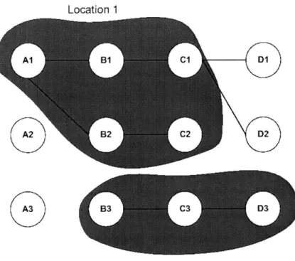
3-1 Cell graph, and significant locations as clusters of individual cell towers

within the graph. . . . . 26 3-2 Bipartite cell graph, with each node representing an hour of the day for

that cell. E.g. Al is cell A at 1 AM. Colored clusters indicate merged locations. . . . . 31

4-1 GPS location clusters and names associated with them. . . . . 34 4-2 Resulting bases from edge-weighted offline algorithm. Arrows indicate

cells that overlap mutliple clusters. . . . . 35

4-3 Transition base consisting of mostly transition cells. . . . . 37

4-4 Base cells for theater cluster. . . . . 38

4-5 Online algorithm bases. Bases are enclosed in black boxes. Larger bases and more single cell bases present were found. . . . . 39

List of Tables

4.1 Average time spans for each base for weekdays and weekends for edge-weighted offline algorithm. . . . . 41 4.2 Percentage overlap for edge-weighted offline algorithm base cells for

given time period, averaged over all weekdays. . . . . 42 4.3 Time spans for bases for Bipartite edge weighted graph algorithm . . 42 4.4 Percentage overlap for base cells for Bipartite edge-weighted algorithm,

Chapter 1

Introduction

The mobile device is the ideal tool for learning patterns of human behavior because it is always with the user. Access to this contextual information allows us to dynamically adapt the application to the user. While location is an important contextual piece on its own, it can also be used as a basis for discovering other contextual information. We believe that relying on GSM-based location discovery, despite its shortcomings, is more desirable compared to other methods since the infrastructure is already in place, and the data can be directly obtained from the mobile device with minimal effort.

1.1

Motivation

Humans are habitual creatures. While we have the potential to be spontaneous, the routines of everyday life usually revolve around the same recurring activities. For example, a typical (week) day might be described as getting up in the morning, breakfast, commuting to work, lunch, and going home. Not surprisingly, the context in which these activities occur, such as time and location, also follow the same pattern of recurrence. If the application can observe and learn these patterns, then the

information presented and actions taken by the application will be more relevant and personalized to individual.

an individual's daily routine that a desktop PC cannot observe simply because the device is usually with the user wherever he goes. As a platform, the mobile device has been widely adopted in nearly every country in the world. Over 800 million cell phones were sold the previous year alone, which translates to one in every six people in the world, dwarfing PC sales

[29].

These advantages make the mobile device the ideal medium for observing and recording the events of everyday life for analysis and learning. The benefits of doing so are as follows:

* Effective querying and viewing of past events, ideally in human terms. For example, the user can ask the application "When was the last time I called my wife when I was in Europe?"

* Provide real time contextual information based on the user's current context to make the overall presentation more meaningful. For example, a tourist guide that shows nearby tourist attractions, such as restaurants, museums, theatres based on the user's current location.

e Dynamically adjust the use of device resources. For example, if we know the

user is moving outdoors from one location to another, then the rate of Bluetooth device scanning can be reduced, which can significantly increase battery life. o Make predictions about user actions on past behavior. For example, instead of

having the user scroll through their entire contact list, present a refined list of people that user is likely to contact based on the current context.

The use of location and time in context aware pervasive computing has been going on for well over a decade, ranging from various location-based services such as Cyber-guide

[15

to personal applications that assist with daily tasks such as Cybreminder

[5] and Place-Its

[23].

However, many of these applications use predefined location infrastructures that are not necessarily personalized to the individual, and often the contextual information is presented in form that is easily processed by a computer, but not necessarily meaningful to the human. A classic example is describing the

user's location in terms of GPS coordinates, as opposed to a more meaningful de-scription such as "workplace". Our goal is to learn how to identify these locations without restricting them to predefined descriptions.

1.2

Location as a Basis for Behavior

This thesis looks at the discovery of significant places that users visit during their typ-ical daily routines using trace logs of GSM cell towers. This discovery process allows us to personalize the information to the individual, rather than using predetermined spots that may not be meaningful to everyone. We then attempt to correlate those locations with time to see how well location can used to determine significant time pe-riods during the day. Since we utilize discovery as opposed to predefined parameters, the results are highly personalized and more meaningful to the individual.

We chose to use cell towers exclusively because the information is readily available almost anywhere without additional hardware or setup, and only requires that the user's device is connected to the cellular network a majority of the time. In contrast, using a more traditional method such as GPS is not as practical since most devices do not include built-in GPS receivers, and those that do require line-of-sight that prohibit them from working well indoors. However, relying on GSM cell traces exclusively has its own drawbacks:

" Cell coverage areas can be very large (several kilometers), especially in

non-urban areas.

" Cells often overlap with each other, so a single location can often see several

cells.

" A one-to-one correspondence between a cell and a location is difficult to

deter-mine due to signal interference

Thus, the accuracy of results obtained using GSM alone can be poor compared to the exact positioning available via GPS. Despite these drawbacks, we found that

using GSM traces alone can still provide a decent approximation of significant places, without relying on sophisticated equipment or expensive data filtering and analysis.

1.3

Outline

In Chapter 2, we describe previous work dealing with collecting and learning be-havioral patterns using mobile devices. We also describe various approaches used to determine location, with focus on GSM-based and hybrid approaches. Chapter 3 looks at the specific algorithms and methodology used in our evaluation, and Chapter 4 describes the results of applying our analysis to an individual's data log over a one month period. Finally, in Chapter 5 we discuss the limitations of our approach and evaluation, and suggest future work and refinements based on what we learned.

Chapter 2

Related Work

This chapter looks at past research in location discovery. We first describe two projects that are particularly relevant to the methods we employed in this thesis, then describe various types of location information used, with emphasis on GSM based approaches.

2.1

ContextPhone

ContextPhone is a cell phone platform developed by the Context Group at the Univer-sity of Helsinki, Finland ((http: //www. cs.helsinki. f i/group/context/) designed to make contextual information readily available to developers. The application runs on conventional Nokia series 60 phones, and has sensors that can detect and log almost every event that occurs on a phone, including GSM and GPS, application status, media capture such as photos taken with the camera, communication such as calls and SMS messages, and devices in the surrounding environment via Blue-tooth [21]. Using this platform the Context Group built several applications. One such application is ContextLogger, which logs the sensor data can then be uploaded via HTTP or Bluetooth periodically in the background for offline analysis, without prompting the user to perform it manually. Another is ContextMedia, which is a file sharing application that can automatically annotate uploaded media with contextual information obtained from the sensors.

The advantages of ContextPhone, namely its ability to record all contextual data available to the cell phone, and its ability to run seamlessly in the background without user interaction make it the ideal platform for observing daily events in a natural setting.

2.2

Reality Mining

The Reality Mining group (http: //reality.media.mit .edu/) at MIT's Media Lab

used a modified version of ContextPhone to record the contextual information of 100 MIT students and faculty over the course of 9 months, amounting to over 350,000 hours of behavioral data as seen from the cell phone. The goal is to provide a rich, expansive data set that can be used explore behavioral patterns on both an individual and group level.

Analysis of the dataset utilized the proximity of Bluetooth devices in many in-stances. For example, Bluetooth IDs were used to detect proximity with other people, and then used to infer actual social relationships between people [8]. Based on this information, a user profile was created, and used as a means of introducing people in proximity that shared similar profile attributes. For location discovery, a hybrid approach correlating cell tower distributions and Bluetooth device distribution was used. For example, cell tower IDs, Bluetooth IDs, and time (hour and weekday vs. weekend) were incorporated in an Hidden Markov Model used to find location clus-ters with accuracy around 95% for some subjects, using predefined dimensions of (office,home,elsewhere) [7]. The results of the analysis were then used to quantify the amount of predictable structure in an individual's life, using an entropy-based metric. Not surprisingly, subjects with "low entropy" tended to have well-defined time periods based on location, while subjects with "high" entropy tended to have

irregular schedules that were much harder to predict.

It is also interesting to note the demographic of the subjects used in the study. The majority were either undergraduate or graduate students who work and live on the MIT campus or surrounding area. Not only is work and home often within a few

minutes walk from each other, but the regular schedule of work hours may not be consistent depending on schedule of classes and student group activities.

2.3

GPS Localization

As described in Section 1.2, the drawback of using GPS-based location discovery methods is their reliance on a GPS receiver and a clear, consistent signal over an extended period. However, under ideal conditions, GPS can provide exact locations with accuracy within several meters. The most common method of identifying loca-tions with GPS readings is by clustering of data points. One common approach was devised by Ashbrook and Starner using a k-means clustering algorithm to identify locations, and further refined those locations by the amount of time the user spent in them

[1].

In comMotion, Marmasse and Schmandt used GPS signal gaps as indication the user entered a significant location, namely a building [17].

Other approaches often incorporate some aspect of Markov modeling and Bayesian filtering. These approaches are often used to predict movement patterns of users, but require significant computation in terms of the modeling and training. For example, Liao et. al. built a hierarchical Markov model using GPS traces, acceleration, and the mode of the cellular device to predict significant outdoor locations where the user changes mode of transportation [14].

2.4

GSM Localization

There exists a significant amount of research on using GSM based location discov-ery. Due to the drawbacks of using GSM based localization, there is a conception that using these approaches is inherently inadequate. Indeed, experimental analy-sis performed by Trevisani and Vitaletti in urban, suburban, and highway environ-ments showed that directly associating the device's location with that of the Base Transceiver Station covering the current cell resulted in differences of 800 meters or more, compared to the actual location recorded via GPS [24]. Based on their analysis,

the authors concluded that direct use of cell IDs for even the simplest location-based services would be inappropriate. Despite this discouraging result, Varshavsky et. al. summarized how past and current research in more advanced GSM localization techniques can obtain sufficient location information appropriate for a wide range of applications that require indoor, outdoor, and place-based location information

[25].

GSM localization methods can be categorized based on the type of signal metric

used and the algorithm employed. In general, the measurements taken include a sub-set consisting of signal strength, signal propagation time, time of arrival (TOA) and time difference of arrival (TDOA), angle of arrival (AOA), and carrier phase

[6].

Once these readings are taken, various types of algorithmic analysis are performed. Some of the more signal-processing intensive techniques include Extended Kalman filters (EKF) [19], hidden Markov models (HMM) [16], and Monte Carlo-based methods

[9]. The methods used in these papers can also be generalized to other kinds of radio

signal networks, such as GPS, WiFi, and conventional AM-FM radio. Accuracy of these signal-processing based methods can vary considerably, ranging from zero to several hundred meters, depending on the type of measurement taken, the amount of noise in the environment, and the frequency of measurement or availability of the particular metric desired. In particular, methods utilizing TOA, TDOA, and AOA require line-of-sight between the receiving device (mobile phone) and the set of base stations. In addition, both TAO and TDAO require synchronized clocks, with the former between base station and device, and the latter between the base stations themselves. The complexity of the analysis and the equipment needed to make the measurements prohibits these algorithms from running on the client side. Further-more, the results are usually more pertinent for the cellular service provider rather than the individual for providing location-based services.

In contrast, GSM localization methods that are geared more to the user's end (client side) rely mostly on the signal strength metric. Additional location informa-tion, such as GPS coordinates, is then used to map the cell towers to physical locations where their signal strength is the strongest. Chen et. al. describe and compare three commonly used algorithmic techniques in this regard - centroid computation,

fin-gerprinting, and Monte Carlo localization with signal propagation [3]. The centroid algorithm simply tries to calculate the center of a set of cells based on GPS coor-dinates as the location value. Fingerprinting utilizes trace logs to detect recurring patterns, and is described in more detail below. The Monte Carlo algorithm is quite similar to signal processing methods described earlier. Of the three, the centroid al-gorithm was the least accurate, while fingerprinting exhibited the highest accuracy in densely populated areas, and the Monte Carlo algorithm in less populated residential areas. Increasing the number of cells used to calculate position improved accuracy significantly in all three cases. Interestingly, Chen et. al. also tested what would happen if the device could scan cell towers from different service providers at the same time. In this case, the Monte Carlo algorithm showed significant improvement, while the fingerprinting algorithm actually performed worse.

Of the algorithms tested by Chen et. al., fingerprinting is by far the most

com-monly used since it is the least dependent on additional location data for support. The algorithm utilizes a trace log of waypoints - in this case, cell towers and their associated parameters such as signal strength or GPS coordinates. It then attempt to determine what the significant places are by detecting the frequency a user revis-its these locations. This process usually involves gathering a large dataset for the training and testing phases.

Laitinen et al. used fingerprints consisting of the 6 strongest cells and a database correlation technique for outdoor localization, and were able to obtain relatively high accuracy in densely populated urban areas [12]. Interestingly, Otason et. al. were able to use GSM fingerprints for localization in an indoor environment as well. They used wide signal strength to include not only the 6 strongest cells, but also up to 29 additional channels that were strong enough to be detected, and were able to obtain results comparable to WiFi-based indoor localization methods [18]. One problem with using wide range GSM fingerprints is that typical cell phone programming interfaces only provide the ID of the current cell tower they are connected to. To obtain the data necessary for these methods, additional equipment such as commercial GSM modems are required.

There are also hybrid approaches that supplement GSM readings with other signal sources (besides GPS) in order to refine some of the inaccuracies of using GSM alone. For example, PlaceLab [13] and BeaconPrint [10] employ both GSM IDs and WiFi Access Point IDs to determine significant locations within a respectable range of accuracy, with the former using premapped beacon locations to physical locations, and the latter introducing an algorithmic approach that does not rely on coordinate-based data. However, most cell phones available today do not have built-in WiFi capability, and the additional drain on battery life of doing WiFi scans continually is particularly costly. The Reality Mining project utilized nearby Bluetooth devices along with GSM logs to determine location (see Section 2.2), but doing so restricts this method to detecting indoor locations exclusively.

To the best of our knowledge, the clique-based fingerprinting algorithm devel-oped by Laasonen et. al. [11] is currently the only GSM localization method that considers cell hand-off patterns, thus requiring no additional hardware and minimal programming to interface with the cell phone. Initial experimental evaluation by Laasonen et. al. showed that their approach does quite well in finding significant locations pertaining to home, work, and leisure. Their approach is particularly at-tractive since the data input required can be readily obtained from ContextPhone as well as simple, home-brewed applications. The simplistic nature of the algorithm also allows it to successfully run online on a cell phone. So far, this technique has been employed successfully on several context-aware applications, including Placelts [23], a location-based cell phone reminder application, and Reno [22], an application for sharing location information among individuals in a social network.

2.5

Other Localization Techniques

One of the earliest location-based systems is the Active Badge system, designed to locate individuals within an office complex by having them wear badges that trans-mit their location to a central server [26]. WiFi signals are also used extensively for location discovery in both indoor and outdoor settings. For example, the RADAR

location system developed at Microsoft utilizes multiple wireless base stations sta-tioned throughout a building and signal propagation modeling to determine a user's location [2]. Cheng et. al. investigated the feasibility of deploying a WiFi network on a city-wide scale, and the accuracy of current WiFi localization algorithms in such a setting with minimal calibration

[4].

Finally, the Cricket location system, which uses strategically placed beacons that transmit radio signals to mobile listener de-vices, introduced a method of location discovery in indoor environments using cheap, off-the-shelf components [20].

Chapter 3

Location and Time Discovery

We present out method for location discovery using GSM trace logs, with entries consisting of a timestamp and the ID of the cell tower the device is connected to. Our method is based on the algorithm devised by Laasonen et. al., but we take advantage of some offline computation in order to be make better informed decisions in the algorithm. Based on the locations discovered, we then correlate them with time periods during the day, averaged over the entire dataset.

3.1

Graph-based Location Discovery

Since the input data consists of timestamped data points, a logical model for the data is a graph of cell transitions, with nodes representing a cell tower, and edges representing the cell phone switching from one cell tower to another. The goal of the graph based approach is to find cluster of cell towers that are "close to each other" and correspond to a significant location, as seen in Figure 3.1.

The key insight provided by Laasonen et. al. is that when the user is at a

location, there is oscillation between several cell towers, meaning the coverage of

those cell towers overlap at that location. However, physical movement back and forth movement often indicates a location of importance, such as an office. Thus, if on average, the time a user spends visiting a cluster is greater than the individual transition times, then there is cell oscillation. Specifically, cell clusters are considered

Coffee shop

k Home

Work

Figure 3-1: Cell graph, and significant locations as clusters of individual cell towers within the graph.

locations if they satisfy the following properties:

1. The subgraph C induced by the cells has max diameter 2.

2. The average length of a visit to a cluster Tagc > |CKmaxTac where JCJ is the number of cells, and max Tavgc is an upper bound on the max length of a transition.

3. Any proper subset of C does not satisfy condition 2.

Condition 1 ensures that cell transitions in a location occur close succession and in a circuitous fashion, thus forming a stable pattern. Condition 2 says that a set of cells is a location if the average time the user spends during a visit is greater than the time spent if the user were to perform a simple walk in the subgraph formed by the location's cells. If there is oscillation among the cells, then additional transition times would be accounted for in Tagc, but not in time for the simple walk. Condition 3 is a minimality condition that tries to ensure locations contain the minimum number of cells required to fulfill conditions 1 and 2, and is an attempt to exclude cells that have large coverage areas.

Significant locations, or bases are then the minimal subset of locations where the user spends a majority of the time.

The definition assumes that when the user is stationary, the set of oscillating cell towers follows a stable pattern. That is, the cell transitions are circuitous, whereas

when the user is on the move, the pattern of cell transitions are more linear. In-tuitively, this assumption makes sense because if the user travels directly from one place to another, the user should also be constantly exiting and entering new cells if he is making consistent forward progress. However, as we found in our evaluation (Chap. 4), these assumptions are not necessarily valid for urban areas with densely positioned cell towers with significant overlapping coverage.

Unfortunately, direct implementation of the definitions proposed by Laasonen et. al. proved to be extremely expensive computationally and impractical for large data sets. The main problem arises from the requirements of conditions 1 and 2. Borrowing terminology from social networking, the subgraphs the algorithm tries to find are essentially n-clubs, which is considered a very difficult problem since they do not enforce the global maximality condition of n-cliques and n-clans [27]. Brute force methods of finding n-clubs are especially intractable for dense graphs such as cell graphs since they require recursive searches for each node in the graph.

3.2

Approximating Locations

The online version of Laasonen et al's algorithm (henceforth referred to as just the online algorithm) used a greedy approximation to the definitions proposed due to the computing resource constraints imposed by cell phone. In the approximation, instead of exhaustively searching for potential clusters, cell clusters are merged incrementally if they satisfy the conditions. We take a similar approach in our offline variant, but take advantage of offline computing resources by building the complete cell graph before hand and calculating time parameters over the entire history of the dataset. The pseudocode for the offline graph building algorithm follows:

Algorithm 1 Build Cell Graph using GSM log. Input is timestamp t and cell tower

c. G is the directed cell graph. t' and c' are the previous timestamp and cell tower. 1: elapsedltime <-- t - t'

2: if elapsed-time < threshhold then

3: if edge(c, c') exists in G then

4: count(edge) <- count(edge) + 1

5: time(edge) <- time(edge) + elapsed-time

6: else

7: add edge(c, c') to G with count = 1 and time = elapsed-time 8: end if

9: end if

In the online algorithm, the total time spent at a location and the number of visits is associated with each cell tower or node in the graph. In our version, we associate the values with each edge transition. Since a location (a subgraph) can be uniquely identified either by its set of nodes or set of edges. By doing so, we reduce the amount of history we need to maintain when computing total and average times since we can just use total sums, whereas using node statistics we would need to partition the total time for each cell based on what percentage was actually spent during visits to this particular subset. We will henceforth refer to this algorithm as the edge-weighted offline version.

The condition on line 2 checks to make sure that there is not a significant gap between consecutive data points (threshold value was set to 1 hour in our analysis). Otherwise, transition times in a cluster might be artificially inflated if the user was actually moving outside of the location, but had the cell phone or logging application turned off.

Once the cell graph is built, the algorithm proceeds to merge cells into locations

by making a second pass through the dataset. The insight here is that since locations

are composed of cells that are "close to each other", they will also appear close to each other in sequentially in time in the GSM trace log. Thus, by looking at a selected window size of cells at a time, we can form the locations incrementally. The

pseudocode for our location merging algorithm follows:

Algorithm 2 Merge cells in cell graph. Input is timestamp t and cell tower c. G is

the directed cell graph. t' and c' are the previous timestamp and cell tower. R is the list of recent locations. s is the maximum size of R.

1: L -- location containing c

2: if L not in R and |R1 >= 2 then 3: merged +- false

4: k +- 2

5: while not merged and k <= R| do 6: m = {ri, ... , rk}

7: if subgraph formed by m satisfies location definition then 8: merge m into new location

9: update R

10: merged <-- true

11: end if

12: k +- k + 1 13: end while

14: if not merged and

JR

= s then

15: remove oldest entry in R

16: end if

17: add new location for c to R

18: end if

The algorithm builds locations from the most recently observed locations. When-ever a new location is encountered, the previous locations are considered for merger if there is a sufficient number. Checking that the subgraph satisfies the necessary con-ditions (line 7) involves calculating the average visit time for the cluster versus the average time for a single tour of the subgraph. These values can be calculated easily using the values associated with the edges in the cluster based on the calculations in Algorithm 1. The average time for cluster is the total time spent transitioning

between cells, divided by the total number of visits. We use a similar weighting func-tion for average times as described in Laasonen et. al. to minimize the impact of cell towers only seen a few times comparatively. The parameter s can impact how locations are merged, since if s is too large, the size of merged locations will also be large. The set of locations returned includes all merged locations, as well as any single-cell locations that were not merged.

Once the set of locations is determined, we sort the set of locations in descending order based on total time spent in them, and select the first n locations that cover a percentage p of the total time. As noted by Laasonen et. al., the choice of p affects the number of bases selected, since if p is too large, then some bases may not actually

correspond to locations that hold any meaning to the user.

One consequence of doing the mergers in this greedy fashion is that if a cell can be associated with multiple locations, it is always merged with the location that is encountered first in the dataset. For example, given locations Li and L2, if cell c can potentially be merged with either, but Li (the cells associated with LI) appeared in the dataset before L2, then c will be merged with L1, and anytime afterwards, c

will always be associated with L1. By forcing cells to be distinct among locations, there is the potential for locations to be too large since they can include cells whose coverage areas actually overlap multiple locations. We attribute this problem to the fact that when building the cell graph, information is lost regarding when in time the cell towers actually appeared together, since we only record aggregate sums of time and visits.

In this fashion, the edge-weighted offline algorithm can produce different locations compared to the online version since the online version merges based on the history of cells seen so far, whereas we utilize the entire history. Using the previous example, in the online version, if cell c was not seen enough times so far to be merged with

L1, but fulfills the definition when associated with L2, then c will be merged with L2 and will be associated with L2 for the duration of execution.

Furthermore, the online algorithm has the potential to produce more single cell locations because the mergers always occur after enough history has accumulated.

Location 1

(A2 B

2D

Location 2

Figure 3-2: Bipartite cell graph, with each node representing an hour of the day for that cell. E.g. Al is cell A at 1 AM. Colored clusters indicate merged locations.

That is, if there is insufficient evidence to validate merging LI with L2 at a particular point even though they could be if we consider the entire history, then Li might be merged with L3 at some later point, and possibly invalidating any possible merger with L2 afterwards.

In order to correct this problem, we devised another scheme, whereby each cell tower node in the graph is divided into 24 duplicate nodes, each one representing the hour of the day. Thus, cell clusters now have a time of day value associated with them. Figure shows 3.2 the type of graph produced.

Mergers between cells and locations now occur between sets of nodes in a bipartite graph. Thus, we effectively split cells that overlap multiple locations, allowing them to be associated with multiple locations as well. This approach will also produce duplicate locations or locations that share a large number of the same cell tower IDs. We resolve this problem by simply merging these locations into a single location once the algorithm completes. Space requirements, however, will most likely increase

dramatically and can be a concern. We will refer to this version as the bipartite edge-weighted offline algorithm.

3.3

Time Period Discovery

After discovering the significant locations or bases, we then correlate those locations with time periods during the day. Our hypothesis is that if the user follows a regular routine each day, then important locations where the user visits can also be used to define significant time periods, or vice versa. Thus, our goal is to see how strong of a correlation there is between location and time, and how well our method of location discovery can be used to discover those time periods.

One approach to accomplish this task is to build a Hidden Markov Model that tries to learn the patterns of association between time and each GSM log event. We instead opted to adopt a simpler approach by observing patterns of cell towers within a specified time window. We proceed sequentially through the logs, looking for sequences of cell towers that correspond to a discovered base. Once found, we continue scanning until we encounter a sequence of cell towers that are either not bases, meaning the user is most like moving from one location to another. This then denotes a significant time period. We maintain a running average of time periods for each base, for time periods that are near other to account for visits to the same location at drastically different times during the day.

One problem that could arise is when during a time window, multiple bases show up, without either having a clear majority. This situation arises if the bases are physically close each other, but were merged separately in Algorithm 1 due to the approximations made. It is unclear what exactly this situation means physically -is the user moving from one location to another, or is he still at a single location, but just happens to be also in range of another location's cell towers? In our evaluation, we chose to interpret this situation as the latter case, given that the physical locations used in our dataset are relatively close to each other.

Chapter 4

Empirical Evaluation

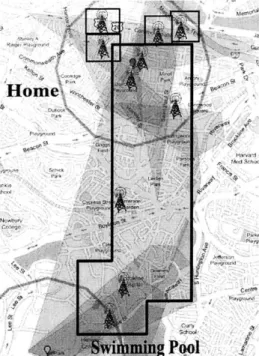
We evaluated the location discovery algorithms using data collected over a one month period on a single subject. The subject's daily routine consists commuting from home to work at MIT's Stata Center during the morning hours, working from the office from midday through the afternoon, and returning home during the evening. The subject also frequently visits recreational locations near his home. The data was collected using a simple, home-brewed Python application than ran on a Nokia 6680 cell phone. Each data point consisted of a timestamp, current GSM tower, and GPS coordinates if the receiver was on. Readings were taken approximately once every 7 seconds and logged to a file for offloading. The log entries were then parsed and stored in a relational database for ease of querying.

4.1

Location Discovery Evaluation

nitial analysis of the dataset was done by Yu to identify significant locations using both GPS and GSM [28]. The analysis used the method developed by Ashbrook and Starner to create the initial clusters, then further refined those locations by calculating

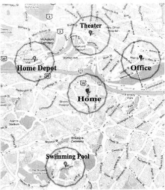
GSM cell coverage polygons. Figure 4.1 shows the locations found by clustering GPS

coordinates, and their corresponding names.

We will use the results of this analysis as basis to judge the accuracy of the locations found using our discovery algorithms.

Theater

4

1ome Depot ,OfficeI

Figure 4-1: GPS location clusters and names associated with them.

4.1.1

Edge-weighted Offline Algorithm Results

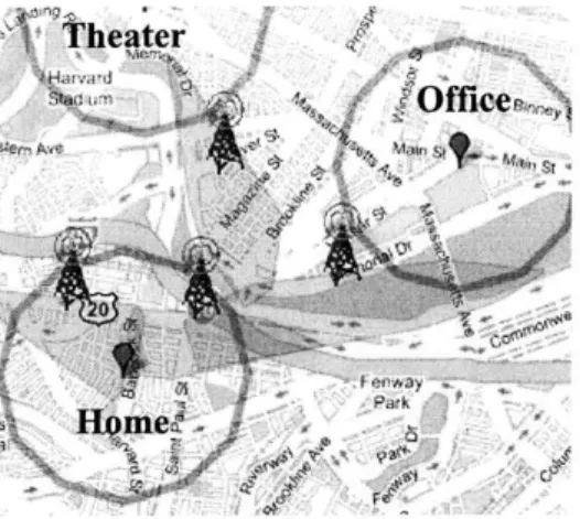
Using the offline algorithm without splitting the nodes based on time, we found 5 bases. Figure 4-2(a) thru Figure 4-2(e) shows how the GSM bases, Base 1-5 re-spectively, correspond to the GPS clusters that were discovered. Note that the pink polygons denote the coverage polygons for each cell tower.

In general, the cell towers for each base were fairly decent in terms of the group-ing. Each cell tower's polygon exhibited some overlap with the base cluster it was associated with. In most cases, the polygons overlapped with a significant portion of the cluster, which agrees with the results found in [28 that these cell towers define the cluster. However, as we noted in the previous chapter, approximations via pair-wise mergers can create bases that are too large. We see this exact situation arise in our results, as can be seen in Figures 4-2(a), 4-2(b), 4-2(d), and 4-2(e). The problem is that these bases include cells (indicated by arrows) that overlap multiple clusters, and thus should have either been included in multiple bases as well, or eliminated altogether.

(a) Base 1 (b) Base 2

(c) Base 3 (d) Base 4

T tm

(e) Base 5

According to Yu's analysis of the dataset, cells such as these indicated with long, narrow coverage polygons indicate transitional cells the device sees when the user moves from one location to another. Due to the close proximity of the various loca-tions in the experiment, these transitional cells were usually still in range when the user arrived at the location, and appeared often enough to satisfy the conditions for merger. In Figure 4-2(d), we see two large transition cells included in the location. In the extreme case almost all of the cells are transition cells like in Figure 4-2(a). These results reveal the flaws in the assumptions make about how a user travels from location to location, using the location definition.

The first assumption is that only when the user is at a base location do the cell towers oscillate in a stable pattern. However, it is conceivable that if the user is in an area where many cell towers are in range, and is moving slowly enough, then the towers may oscillate in a stable pattern as well, particularly if the user is moving between locations in close proximity. Thus, over time, if the user moves along this path often enough, the transition edges between these towers will accumulate enough time to actually fulfill the definition of a location. In Figure 4-2(d)'s case, the subject often commutes between home and office via bicycle at a steady pace.

In Figure 4-2(a)'s case, while the subject commutes between home and the swim-ming pool via car, the actual route that was taken was non-linear. That is, the route included numerous back and forth turns. Thus, actual forward, linear progress is far less compared the total time spent going back and forth, the cell hand-off patterns can once again exhibit stable oscillation. Once again, close proximity between the

starting location and destination makes this situation even more likely to occur. Unfortunately, we were unable to discover any base corresponding to the "The-ater" GPS cluster. Most likely this is due to the low number of times that particular location was visited compared to others, since our algorithm tries to minimize the impact of cell towers that are only seen a few times via weighting. It is also interesting to note that the choice of parameter p had minimal impact on the resulting bases.

Again, we attribute this phenomenon primarily to the sparseness of the data that was collected.

VI

-*

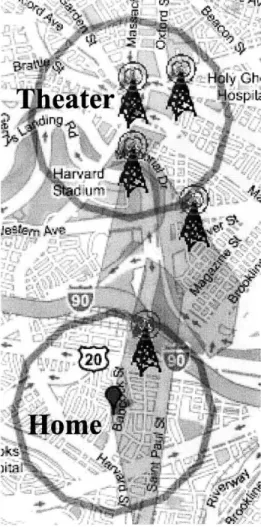
Figure 4-3: Transition base consisting of mostly transition cells.

4.1.2

Bipartite Edge-Weighted Offline Algorithm Results

Next, we looked at the bases that were found if we used time division nodes in the cell graph. While we expected this version to take considerably longer to execute, in reality running time was about the same as the non-bipartite version. Again, since our dataset is rather sparse, even though there are considerably more nodes in the graph, the number of edge transitions is still quite small. The bases found by the algorithm were also smaller on average in terms of the amount of area covered by the cells, and several bases included copies of the same cell, achieving the desired effect. Specifically, there were several bases that covered the home cluster which could conceivably be merged together. Unfortunately, due the size of coverage areas for some cells, we were unable to completely exclude transition cells. For example, the coverage of cells in the area between "Home" and "Swimming Pool" are quite large, and appeared as bases in multiple instances. However, in general, there was better separation between cluster bases and transition bases, as can be seen in Figure 4.1.2. Interestingly, the algorithm also identified a base that corresponds to the theater as seen in Figure 4.1.2. Most likely this base emerged because of multiple copies of the same node available for merger. These additional nodes allowed the other cells in the Theater cluster to merge successfully to satisfy the location definition, whereas previously those cells were merged with other locations and unavailable later on for consideration.

Figure 4-5: Online algorithm bases. Bases are enclosed in black boxes. Larger bases and more single cell bases present were found.

However, we were unable to obtain a base for the "Home Depot" cluster. We attribute this shortcoming to the fact that the "Home Depot" cluster appeared only once or twice in the dataset, and at different enough times such that without an aggregate, we the time stayed at the location was insufficient. The complete set of bases found can be found in Appendix A.

4.1.3

Online Algorithm Results

For comparison sake, we also ran Laasonen et. al.'s online algorithm on our dataset. The results were rather inconsistent. The online algorithm found significantly more bases. In some instances the bases were quite large, but many also consisted of only single cells. We described how this situation can arise in Section 3.2. In our dataset, this situation occurred fairly often because there were significant time gaps between a set of readings. Thus, during any particular iteration, transitions may not have occurred enough times or even at all to validate merger between cells. Figure 4.1.3 shows a partial view of the bases found.

It is not surprising that the online algorithm did not perform as well as the offline variants. Since it is designed to run in real time, it must make decisions based on limited information, so that given a sparse and inconsistent dataset, it has even less information to work with.

4.2

Time Correlation Evaluation

To correlate location with time, we scanned through the dataset sequentially based on time and record time spans where the sequence of cell towers corresponds to a base. We then compared the results of the regular and bipartite cell graph algorithms. We include in the appendix average time spans per day for each base for both algorithms.

A major issue we encountered while performing the scanning is due to close

phys-ical proximity of the various locations, often cells associated with one location are in range fairly consistently even though the user is in another location. The edge-weighted offline algorithm was especially susceptable. Cells associated with Base 1

(Swimming Pool) overlapped significantly with cells in Base 2 and to some extent in Base 4. Therefore, time spans when the user is actually at home, during the evening and overnight hours are included in Base 2's average time spans. This issue impacted results more in the regular cell graph than the bipartite one.

A second issue encountered is that the dataset contains significant gaps of several

hours in time between one reading and the next caused by the user turning off the application or phone, or losing signal while indoors. This issue occurred often enough such that using our initial approach of using the exact times when base cells were observed and not observed resulted in time spans that were extremely short and far apart. Without additional data or analysis to fill in these gaps, we handled this case

by buffering start and end times for the spans by a proportion of the gap time.

4.2.1

Edge-Weighted Offline Time Periods

Average time spans over individual days were fairly inconsistent, with some days even lacking time information for certain bases. However, if we instead look at the time

Weekday Weekend Base 1 7:54 - 14:36 7:29 - 14:54 Base 2 6:43 - 19:21 4:54 - 20:14 Base 3 11:46 - 19:11 12:54 - 17:13 Base 4 9:27 - 15:56 5:18 - 8:16 Base 5 4:06 - 12:58 9:28 - 16:46

Table 4.1: Average time spans for each base for weekdays and weekends for edge-weighted offline algorithm.

spans on a larger scale, namely weekday versus weekend, the average time spans tend to distinguish a little more, as shown in Table 4.1. Specifically, on weekdays the subject spends mornings and evenings around his residential area (Base 1, Base 2,

and Base 4), and works from his office during the midday and afternoons (Base 3). The results for Base 5 are rather inconsistent due to the large transition cell included between Home and Home Depot. The results for the weekend appear more arbitrary, and are difficult to interpret since the subject does not have a particular routine that he follows during those days. However, times for Base 5 appear more consistent for when visits are made to the shopping center.

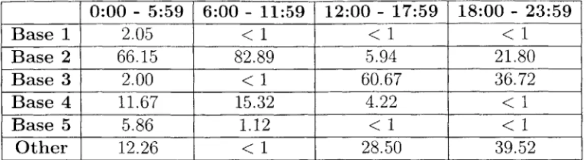
We then looked how much contribution each base makes during set time periods of morning, midday-afternoon, and evening. The goal is to determine whether the overlaps are significant, or caused by just a few towers from a neighboring location that happens to be in range. The results are shown in Table 4.2.1 averaged over all weekdays. The "Other" row is a useful indication of when the subject is poten-tially moving from one location to another, or a base that our algorithm did not discover. Note in our analysis, the time period 6:00-11:59 significantly fewer data points compared to the others.

From these values, we can see that Base 2 seems to provide a good indicator of when the subject is home, and Base 3 for when the subject is at the office, which supports the results we obtained earlier. Base 4 supports our previous conjecture that is more of transition base. Base 1 and 5 appear very infrequently in the dataset, so that even though their time spans overlap quite a bit with the other time spans, they can be disregarded. In three of the four time periods, other cell towers appear

0:00 - 5:59 6:00 - 11:59 12:00 - 17:59 18:00 - 23:59 Base 1 2.05 < 1 < 1 < 1 Base 2 66.15 82.89 5.94 21.80 Base 3 2.00 < 1 60.67 36.72 Base 4 11.67 15.32 4.22 < 1 Base 5 5.86 1.12 < 1 < 1 Other 12.26 < 1 28.50 39.52

Table 4.2: Percentage overlap for edge-weighted offline algorithm base cells for given time period, averaged over all weekdays.

Weekday Weekend Base Home 8:42-12:39, 16:50-20:34 7:45 - 13:20 Base Home-Pool 5:53 - 7:55 8:43 - 11:00 Base 2 9:24 - 12:50 9:50 - 13:00 Base 4 11:04 - 15:14 7:24 - 14:42 Base 5 7:42 - 16:00 12:54 - 15:27 Base 7 9:26 - 11:37 8:32 - 11:40

Table 4.3: Average time spans for bases for Bipartite edge weighted graph algorithm.

a significant amount of time, and in the last period, they occur the most often. It is quite possible that some of bases are missing cells that should have been included, but it is also the result of the dataset representing a relatively small physical area with densely populated cell towers.

4.2.2 Bipartite Edge-Weighted Offline Time Periods

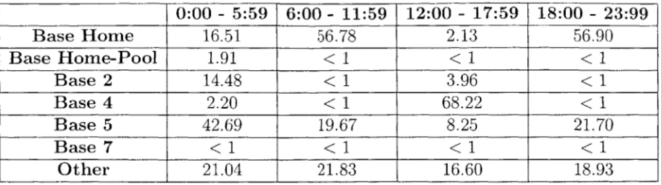
Since the output of the bipartite cell graph algorithm contained bases that shared many of the same cell towers, the time spans for bases overlap ever more. However, the time spans are also significantly shorter given the smaller base sizes. Appendix B lists the time spans for all 8 bases. To make the time spans more distinct, we merged bases that shared a majority of the same cells and preferably contained no transition cells. Specifically, Base 1 and Base 8 were merged into "Base Home", while Base 3 and Base 6 were merged into "Base Home-Pool". Table 4.2.2 shows the time spans for the bases after the mergers.

0:00 - 5:59 6:00 - 11:59 12:00 - 17:59 18:00 - 23:99 Base Home 16.51 56.78 2.13 56.90 Base Home-Pool 1.91 < 1 < 1 < 1 Base 2 14.48 < 1 3.96 < 1 Base 4 2.20 < 1 68.22 < 1 Base 5 42.69 19.67 8.25 21.70 Base 7 < 1 < 1 < 1 < 1 Other 21.04 21.83 16.60 18.93

Table 4.4: Percentage overlap for base cells for Bipartite edge-weighted algorithm, averaged over all weekdays.

the results from the normal cell graph in Table 4.1. In particular, Base Home showed two distinct time spans as opposed to one continuous span. Base 2 also appears as a possible candidate for merging with Base Home. Base 5 is the only base that still covers a large time span, but since it's cells overlap with 2 other location clusters, we would expect it to do so.

Finally, we look again at the percentage of cell overlap for certain time periods. Table 4.2.2 shows these values.

First, we see how Base Home more clearly defines the morning and evening time periods when the subject is commuting to or from home or is at home. Second is that the transition Base 5 appears fairly consistently across all time periods for long durations. This result is consistent with the large, overlapping cells contained in base

5. Finally, looking at the "Other" row, compared to Table 4.2.1, the amount of time

spent in range of non-base cells is consistent across all time spans. Since the bipartite cell graph produced time spans that were shorter in duration, but more disjoint, these extra cells were consistently seen to "fill" the gaps in time.

Overall, it appears that the bipartite graph algorithm produces more desirable results, with respect to some of the nuisances of the dataset we worked with.

Chapter 5

Limitations and Future Work

One major limiting factor in our experimental evaluation was the sparseness of the dataset. Not only did the dataset only cover a single month, it also contained signifi-cant gaps in time between readings that required the use of time padding. Despite the algorithms giving decent results, evaluation with a more extensive dataset covering a longer period time is needed to further test its effectiveness.

Another issue is our limited ability to verify the correctness of the locations discov-ered. In our evaluation, we used previous analysis that incorporated GPS information as well for verification. However, if we were to evaluate a larger dataset that contained only timestamps and cell tower IDs, then correctness can really only be judged with direct verification with the user. This issue also arises if attempt to apply our ap-proach to the Reality Mining dataset, since it also does not contain GPS coordinates, though it does include names that the subjects gave to specific cell towers.

We noted in our evaluation how proximity of locations and density of cell towers can impact the results of the algorithm. It would be interesting compare the algo-rithm's performance by varying these factors. Also, since we knew ahead of time that the subject tended to follow a regular schedule, we could try to determine how much variation the algorithm allows for before results deteriorate considerably.

Since Laasonen et. al. intended to run their algorithm in real-time on the cell phone, it would be interesting to see how locations could be restructured if it were given bases that were discovered first in offline analysis.

While we tried to personalize the information by not associating locations with descriptions that are not meaningful to a human, the next step would be to learn meaningful descriptions for locations and time periods automatically without prompt-ing the user every time this information is needed. At the very least, we could learn when it is convenient to ask the user such questions, based on their current context.

In this thesis, we looked at correlating location with time. However, there are numerous other types of contextual information that could be correlated. For ex-ample, if we assume people routinely do the same things again and again, then we can assume that they also tend to call the same people routinely while they are at a certain location. This could also be applied to what applications they us and what people they come into contact with. In this thesis, we attempted to correlate location with time. It would interesting to see also if whether a dependency relationship can be establish. That is, whether time is dependent on location or vice versa for the user. Doing so could produce more accurate predictions and also help fill in missing contextual information or reinforce existing information.

Chapter 6

Conclusion

The cell phone is more than just a portable phone. It is a feature-rich platform that can be used to learn things about the user and adapt dynamically in ways conventional PCs cannot. One of most important distinctions is the mobile device's ability to take into account real-time contextual information since it is almost always with the user. We showed how by using conventional phone interfaces and some simple graph analysis, we can determine locations that a user frequents, and then correlate that with time to discover important time periods during a day's routine. The more we can learn about the patterns of user behavior, the more we can truly make mobile computing human-centric.

Appendix

Bases for Bipartite Edge-Weighted

Algorithm

(b) Base 2

(c) Base 3 (d) Base 4

(a) B ase 1

IL 4! o d

(e) Base 5 (f) Base 6

Appendix B

Time-span average results

B.1

Edge-weighted algorithm

Monday: Base 1:('02:24:00', Base 3:('16:32:00', Base 2:('10:33:00', Base 5:('03:06:00', Base 4:('10:43:00', Tuesday: Base 1:('07:47:00', Base 3:('12:14:00', Base 2:('07:00:00', Base 5:('04:21:00', Base 4:('10:15:00', Wednesday: Base 1:('12:47:00', Base 3:('10:03:00', Base 2:('03:49:00', Base 5:('02:43:00', Base 4:('08:29:00', '08:10:00') '23:51:00') '19:54:00') '15:10:00') '14:15:00') '14:18:00') '18:18:00') '20:33:00') '15:42:00') '15:44:00') '19:21:00') '17:41:00') '19:30:00') '11:17:00') '17:52:00')

Thursday: Base 3:('08:58:00', Base 2:('08:06:00', Base 4:('10:39:00', Friday: Base 1:('06:51:00', Base 3:('14:01:00', Base 2:('03:52:00', Base 5:('06:04:00', Base 4:('07:53:00', Saturday: Base 1:('08:56:00', Base 3:('11:52:00', Base 2:('01:21:00', Base 5:('08:16:00', Base 4:('09:11:00', Sunday: Base 1:('02:23:00', Base 3:('18:00:00', Base 2:('11:19:00', Base 5:('00:53:00', Base 4:('10:11:00', '19:32:00') '19:46:00') '18:47:00') '14:37:00') '19:31:00') '16:42:00') '12:15:00') '13:55:00') '16:24:00') '16:37:00') '19:20:00') '11:20:00') '15:50:00') '09:37:00') '20:16:00') '21:50:00') '03:39:00') '19:05:00')

B.2

Bipartite edge-weighted algorithm

Monday: Base 8:('00:27:00', Base 1:('12:46:00', Base 3:('10:44:00', Base 2:('12:41:00', Base 5:('10:54:00', Base 4:('13:52:00', Base 7:('18:58:00', Base 6:('10:44:00', Tuesday: Base 8:('16:17:00', Base 1:('13:42:00', Base 3:('11:57:00', Base 2:('13:53:00', Base 5:('15:51:00', Base 4:('13:02:00', Base 7:('11:28:00', Base 6:('11:57:00', Friday: Base 8:('13:15:00', Base 1:('15:41:00', Base 3:('15:12:00', Base 2:('15:13:00', Base 5:('14:48:00', Base 4:('13:53:00', Base 7:('18:19:00', Base 6:('15:12:00', Wednesday: '00:43:00') '16:14:00') '12:20:00') '14:56:00') '13:10:00') '17:08:00') '23:59:00') '12:20:00') '20:06:00') '15:39:00') '16:13:00') '16:13:00') '18:42:00') '19:44:00') '12:50:00') '16:13:00') '17:06:00') '19:58:00') '19:02:00') '20:39:00') '19:07:00') '21:18:00') '21:42:00') '19:02:00')