HAL Id: halshs-01223321
https://halshs.archives-ouvertes.fr/halshs-01223321
Preprint submitted on 2 Nov 2015
HAL is a multi-disciplinary open access archive for the deposit and dissemination of sci-entific research documents, whether they are pub-lished or not. The documents may come from teaching and research institutions in France or abroad, or from public or private research centers.
L’archive ouverte pluridisciplinaire HAL, est destinée au dépôt et à la diffusion de documents scientifiques de niveau recherche, publiés ou non, émanant des établissements d’enseignement et de recherche français ou étrangers, des laboratoires publics ou privés.
Parents’ education and child body weight in France:
The trajectory of the gradient in the early years
Bénédicte H. Apouey, Pierre-Yves Geoffard
To cite this version:
Bénédicte H. Apouey, Pierre-Yves Geoffard. Parents’ education and child body weight in France: The trajectory of the gradient in the early years. 2015. �halshs-01223321�
WORKING PAPER N° 2015 – 36
Parents’ education and child body weight in France: The trajectory
of the gradient in the early years
Bénédicte H. Apouey
Pierre-Yves Geoffard
JEL Codes: I12
Keywords: Children; BMI-for-age z-score; Body Weight; Overweight;
Socioeconomic Status; Education
P
ARIS-
JOURDANS
CIENCESE
CONOMIQUES48, BD JOURDAN – E.N.S. – 75014 PARIS
TÉL. : 33(0) 1 43 13 63 00 – FAX : 33 (0) 1 43 13 63 10
www.pse.ens.fr
CENTRE NATIONAL DE LA RECHERCHE SCIENTIFIQUE – ECOLE DES HAUTES ETUDES EN SCIENCES SOCIALES ÉCOLE DES PONTS PARISTECH – ECOLE NORMALE SUPÉRIEURE – INSTITUT NATIONAL DE LA RECHERCHE AGRONOMIQUE
Parents’ education and child body weight in France:
The trajectory of the gradient in the early years
B´en´edicte H. Apouey, Pierre-Yves Geoffard October 30, 2015
B´en´edicte H. Apouey (corresponding author)
Paris School of Economics - CNRS, 48, Boulevard Jourdan, 75014 Paris, France. Phone: 33-1-43-13-63-07.
Fax: 33-1-43-13-63-55.
E-mail address: benedicte.apouey@psemail.eu; benedicte.apouey@gmail.com.
Pierre-Yves Geoffard
Paris School of Economics - CNRS, 48, Boulevard Jourdan, 75014 Paris, France. E-mail address: pierre-yves.geoffard@psemail.eu.
ABSTRACT
This paper explores the relationship between parental education and offspring body weight in France. Using two large datasets spanning the 1991-2010 period, we examine the existence of inequalities in maternal and paternal education and child reported body weight measures, as well as their evolution across childhood. Our empirical specification is flexible and allows this evolution to be non-monotonic. Significant inequalities are observed for both parents’ education – maternal (respectively paternal) high education is associated with a 7.20 (resp. 7.10) percentage points decrease in the probability that the child is reported to be overweight or obese, on average for children of all ages. The gradient with respect to parents’ education follows an inverted U-shape across childhood, meaning that the association between parental education and child body weight widens from birth to age 8, and narrows afterward. Specifically, maternal high education is correlated with a 5.30 percentage points decrease in the probability that the child is reported to be overweight or obese at age 2, but a 9.62 percentage points decrease at age 8, and a 1.25 percentage point decrease at age 17. The figures for paternal high education are respectively 5.87, 9.11, and 4.52. This pattern seems robust, since it is found in the two datasets, when alternative variables for parental education and reported child body weight are employed, and when controls for potential confounding factors are included. The findings for the trajectory of the income gradient corroborate those of the education gradient. The results may be explained by an equalization in actual body weight across socioeconomic groups during youth, or by changes in reporting styles of height and weight.
HIGHLIGHTS
• We examine the gradient in parental education and reported child body weight across childhood.
• Maternal high education is associated with a 7.20 percentage points decrease in child overweight.
• Our specification allows the evolution of the gradient to be non-monotonic with child age.
• The gradient follows an inverted U-shape with age: maternal high education is correlated with 5.30, 9.62, and 1.25 percentage points decreases in child overweight at ages 2, 8, and 17, respectively.
• The results suggest an equalization in body weight or a change in reporting style in youth.
JEL classification: I12.
Keywords: Children; BMI-for-age z-score; Body Weight; Overweight; Socioeconomic
1
Introduction
The overweight rate among youth is relatively low in France and it has remained stable between 1990 and 2006. However, recent trends in overweight for boys are a public health concern: their rate of overweight has increased by 2.8 percentage points between 2006 and 2010. In 2010, around 15% of children were overweight (OECD, 2014). Overweight reduces quality of life in the physical, emotional, social, and school functioning domains (Schwim-mer et al., 2003). In addition, overweight in childhood has adverse health consequences in adulthood, including diabetes, cardiovascular diseases, some cancers, and premature mor-tality (Reilly and Kelly, 2011). There is also some evidence that overweight is associated with lower skills attainment, although this result is mixed (Murasko, 2015; Palermo and Dowd, 2012). Finally, overweight in the early years is associated with poorer labor market outcomes (Sargent and Blanchflower, 1994). Therefore, the importance of understanding the determinants of child body weight is clear.
Family socioeconomic status (SES) tends to be inversely related to child body weight (Apouey and Geoffard, 2014; Costa-Font and Gil, 2012; Murasko, 2009; Steckel, 1995).
This association may be explained by two mechanisms.1 First, SES may have an impact
on body weight, for instance if low-SES families are more likely to buy high-fat, energy-dense foods because they are less expensive (Drewnowski and Specter, 2004), or if low-SES individuals live in neighborhoods in which access to healthy food is limited (Baker et al., 2006). Second, the association between family SES and child body weight may be an artefact due to the omission of third factors, such as genetics.
The evolution of the gradient in family SES and child body weight over childhood is a rather unexplored topic. On the one hand, one could expect that the association between SES and body weight increases with age. That will be the case if body weight develops over long periods and reflects the cumulative effect of family SES. On the other hand, the increase in social inequalities across childhood may not be irreversible. Indeed, older children and adolescents may progressively detach themselves from their parents and
1
Child body weight should only have a limited effect on family SES. Suppose that our SES variable of interest is education. Note first that in France, people tend to have children after they leave the education system – in 2010, parents have their first child at age 28 (INED, 2010), which is a long time after they finish full time education. Note also that among the small proportion of young parents who stop going to school, the share of those who do it because of their child weight must be limited. As a consequence, we expect the impact of child body weight on parents’ education to be negligible. On a related issue, the literature on the gradient in family income and child general health has established that the impact of child general health on family income is statistically small and only explains a very small share of the gradient (Apouey and Geoffard, 2013; Case et al. 2002).
spend more time with their peers. As a result, they may all be influenced by the same social norms regarding ideal body weight irrespective of their family SES, and low-SES children may be actively controlling their body weight to lose weight, which would lead to a decrease in the gradient with age. Using data on children ages 2-19, Murasko (2009) finds that the association between income and obesity is stable with age in the US. In a sample of individuals transitioning from early to middle adulthood, Baum and Ruhm (2009) find that the gradient in maternal education and offspring body weight widens with offspring age in the US. This implies that the negative effect of poor maternal education accumulates over child lives. This result is consistent with previous findings on child general health by Case et al. (2002), who highlight that the correlation between family income and child general health strengthens as children grow older in the US.
Our article asks whether family SES matters for child body weight, and how the relationship between SES and child body weight changes as children get older in France. Our data come from two surveys, the Survey on Health and Medical Care (“Enquˆete sur la Sant´e et les Soins M´edicaux” – ESSM) for 1991-1992 and 2002-2003 on the one hand, and the Health, Health Care, and Insurance Survey (“Enquˆete sur la Sant´e et la Protection Sociale” – ESPS) for 1996-2010 on the other hand, which contain approximately 40,000 observations of children in total.
Family SES can be defined in a number of ways, using for instance education, income, wealth, or profession. Education and income capture slightly different aspects of family SES: education by itself may be related to social norms, awareness, knowledge, and access to information, whereas income should capture the ability to pay. This explains why in the published literature the trajectories of the education and income gradient are sometimes different: in Case et al. (2002) for instance, the gradient in education and child general health is stable as children grow older, while the gradient in income strengthens with age. In this paper, we focus on parents’ education and we measure it in two different ways. However, we also present results on income, which are consistent with those on education but are less robust (see Section 4.2.1).2
There are two types of anthropometric data: in the objective approach, height and 2
We focus on education rather than income for several reasons. First, even if our results on income and education are consistent, the findings on education are clearer and more robust. This might be due to measurement error in the income variables. Second, for space reasons. Third, although we are not aware of any study that compares the role of income with that of education on child body weight in France, there is some suggestive evidence that education matters more than income in explaining body weight. Indeed, a report argues that education is a stronger determinant of diet quality than income in France (Recours and Hebel, 2006).
weight are measured, whereas in the subjective approach, height and weight are self-reported. Reported data are important because they capture how people perceive their body, and perceived body weight will have an influence on weight control, eating behaviors, and physical activity – individuals who do not perceive that they are obese won’t try to lose weight. The ESPS and ESSM surveys contain reported data, and using these piece of information, we compute child body mass index (BMI)-for-age z-score and a dichotomic variable for whether the child is overweight or obese.
To uncover the evolution of the gradient across childhood, we start by investigating the correlation between parents’ education and child body weight separately by child age groups, using the ESSM data. The results enable us to develop a specification that ac-counts for the shape of the gradient across childhood. We then examine whether this shape is statistically significant using the large sample of children of all ages. Overall, our em-pirical specification allows for the possibility that during childhood there may be periods of convergence among children from diverse social environments, followed by periods of divergence, or the contrary. In other words, we account for the fact that inequalities may not monotonically increase with age, which means that they may not necessarily be cumu-lative. In further analysis, we investigate whether our results are robust to the inclusion of potential confounding factors (e.g. parents’ labor market status, family income, and parents’ body weight). At the same time, we look at the trajectory of the income gradient. We also re-estimate our model (for education) including cohort or child fixed effects, since the age-profile of the gradient may be obscured by cohort or child characteristics. In a subgroup analysis, we examine the gradient separately by child gender and survey year.
This paper contributes to the literature on social disparities in body weight and health in the early years on several fronts. First, we contribute to the literature on health inequal-ities in France. In 2000, Anne Tursz lamented that knowledge on the relationship between social environment and child health in France was limited and we are under the impression that only little progress has been made since then (Tursz, 2000). In particular, the existing literature on the gradient in childhood uses data from specific child age groups or specific regions (Currie et al., 2012; Guignon and Bad´eyan, 2002; Kaminski and Saurel-Cubizolles, 2000; Klein-Platat et al., 2003), with very few exceptions (Apouey and Geoffard, 2014, 2015). It is thus an open question whether the findings can be generalized to all French children. In contrast, in this article, we study inequalities using two nationally representa-tive samples of French children, which hopefully enables us to get general results. Second,
by focusing on France, we also complement the literature on the evolution of the social gradient in child anthropometric measurements across childhood, which has solely focused on the UK and the US so far. Indeed, the results for the UK and the US may not hold in France because the health care system is different,3 the prevalence of overweight and
obesity is smaller,4
and social norms are probably stronger in France.5
Third, to uncover the evolution of the gradient across childhood, we use an econometric specification that allows the impact of parental education on child outcomes to be non-monotonic with child age. In contrast, the recent literature often assumes that the gradient in body weight is a monotonic function of child age. Fourth, we study the impact of paternal education on child body weight outcomes in addition to maternal education. Previous research has generally investigated the role of the mother’s education only.
2
Background
A negative association between economic conditions and child body weight is found in most developed countries (Classen and Hokayem, 2005; Murasko, 2009, 2011; Zhang and Wang, 2006). In what follows, we only present the small number of papers that focus on France. Using data on children ages 2 to 17 from the 1996-2010 waves of the ESPS, Apouey and Geoffard (2014) highlight that family income is negatively correlated with child BMI-for-age and overweight status. For a sample of 30,000 children ages 5 and 6 in 2000-2001, Guignon and Bad´eyan (2002) show that children living in poorer areas are more likely to have weight problems. Employing a dataset containing 2863 adolescents aged 12 from the Department of Bas-Rhin in 2001, Klein-Platat et al. (2003) highlight that the mother’s educational level and the family income tax level are negatively and significantly correlated with the probability of overweight or obesity, whereas the father’s educational level is not.6 Finally, in the 2009-2010 Health Behaviour in School-Aged Children (HBSC)
3
France has a mixed public-private social insurance system, and private insurance provides cover against public sector co-payments on prescription medicines and dental care in particular; in the UK, the system is public and tax-financed; and in the US, the system is predominantly private.
4The share of overweight or obese children is 13.1% for boys and 14.9% for girls in France (in
2006-2007, for children ages 3-17, using the IOTF standards), 35.6% for boys and 36.3% for girls in Eng-land (in 2013, for children ages 11-15, using the 85th percentile cut-off), 33.6% for boys and 27.4% for girls in Scotland (in 2012, for children ages 2-15, using the 85th percentile cut-off), and 35.1 for boys and 33.2 for girls in the US (in 2009-2010, for children ages 5-17, using the IOTF standards). See http://www.worldobesity.org/site media/library/resource images/Child Global 10th June 2015 WO .pdf
5
Indeed, for adults, ideal body weight is smaller in France than in the UK (for both men and women) and underweight is considered in a more positive light in France than in the UK (for women) (De Saint Pol, 2009b).
study, adolescents from less affluent families are more likely to be overweight or obese (Currie et al., 2012).
The evolution of the gradient in family SES and body measures across childhood is a rather unexplored topic, and the literature has only focused on the UK and the US so far. Howe et al. (2013) use data on a cohort of British children born in 1991-1992 from the Avon Longitudinal Study of Parents and Children. They demonstrate that maternal education differences in offspring total body fat mass (assessed by whole body dual x-ray accelerometry scan) is significant and increases with age for females, while it is insignificant and stable for males. Using cross-sectional data on children ages 2-19, Murasko (2009) finds that the association between income (measured by the poverty-to-income ratio) and obesity is stable with age in the US. Murasko (2013) exploits longitudinal data on US children ages 6 to 14 from the Early Childhood Longitudinal Study, 1998-1999 Kindergarten Cohort (ECLS-K), to examine the gradient in BMI (and height). His results suggest that the impact of (the log of) income on BMI decreases (linearly) with age. Of particular relevance is also research by Baum and Ruhm (2009): using data from the National Longitudinal Survey of Youth (NLSY) on individuals moving through early adulthood, these authors show that disparities in obesity increase (linearly) with age in the US, which is consistent with an age-pattern during childhood.
This literature provides evidence on the evolution of the gradient in the UK and the US, and one can wonder whether the results are universal. In addition, some of these articles use a model that regresses child outcomes on family SES, child age, an interaction term between family SES and child age, and controls, which tests whether the association between family SES and child outcomes monotonically increases or decreases with age
(Baum and Ruhm, 2009; Murasko, 2013).7
In this paper, we complement the previous literature by using data for France and allowing the evolution of the gradient in parental SES and child outcomes to be non-monotonic.
3
Data and methods
3.1 The ESSM and the ESPS
Our primary data source is the ESSM for 1991-1992 and 2002-2003. In 1991-1992, the sur-vey was carried out by the “Institut National de la Statistique et des Etudes Economiques”
7
The model does not include an interaction term between family SES and higher order polynomials of child age.
(INSEE) and the “Centre de Recherche, d’Etudes et de Documentation en Economie de la Sant´e” (CREDES), and in 2002-2003, the survey was carried out by the INSEE. The survey is cross-sectional and it is done every ten years approximately – the 1991-1992 and 2002-2003 surveys are the two most recent waves. The data are collected by face-to-face interviews and self-completion questionnaires. To our knowledge, the ESSM data have been used to study social inequalities in body weight in adulthood (De Saint Pol, 2009a; Etil´e, 2014; Singh-Manoux et al., 2010), but not in childhood yet.
We complement the ESSM with the ESPS data between 1996 and 2010. The exact survey years are 1996, 1997, 1998, 2000, 2002, 2004, 2006, 2008, and 2010.8
The survey is carried out by the “Institut de Recherche et Documentation en Economie de la Sant´e” (IRDES) and the “Caisse Nationale de l’Assurance Maladie des Travailleurs Salari´es” (CNAMTS). The survey is a rotating panel, and some households are re-interviewed ap-proximately every four years. However the number of children that are actually followed over time is small, and consequently we pool all the waves and do not take advantage of the longitudinal nature of the data in our main specification. We exploit the longitudinal aspect of the ESPS in a robustness check though. The data are collected by a combination of phone interviews, face-to-face interviews, and self-completion questionnaires.
To our knowledge, these surveys provide the two largest samples containing children of all ages matched with their parents for France. The samples are representative of French households. In this paper, we define a child as an individual aged 0-17, who is the child of the respondent or his partner. The ESSM sample contains 14,080 children, and the ESPS sample, 24,908 observations.
Note that the ESSM contain less observations than the ESPS. However, the questions on education are consistent across waves in the ESSM, allowing us to create for each parent two education variables, whereas they are not in the ESPS, which explains why we are only able to create for each parent one education variable that suffers from measurement error (see Section 3.2.2). This is the reason why the ESSM data is our preferred dataset in this analysis.
8
We do not use the 1994 wave of the ESPS because there is no information on the month when the child height and weight are reported.
3.2 Variables
3.2.1 Reported child body weight
Both surveys contain child reported height and weight. Height and weight are reported by the parents in the ESSM data, and either by the parents or by the child (or by an
unknown household member) in the ESPS data.9
We use information on the child height and weight, gender, and age in months at the time of the interview, to derive the gender- and age-adjusted BMI-for-age z-scores, using the “zanthro” Stata function (Vidmar et al., 2013) with the WHO reference growth chart. The Stata “zanthro” function allows to use the WHO, UK, or US growth reference chart. We chose the WHO reference because our study is for France and so international standards seem more appropriate. The WHO growth chart uses the “WHO Child Growth Standards” and “WHO Reference 2007” composite data files as the reference data. The “WHO Child Growth Standards” are the result of the Multicentre Growth Reference Study, which focuses on children ages 0-5 years and contains growth data on infants and young children from Brazil, Ghana, India, Norway, Oman, and the US. The “WHO Reference 2007” contains information on children and adolescents ages 5-19.
In addition, we create two dummy variables for whether the child is overweight or obese, using the cut-off points of the WHO and of the IOTF. To create the overweight or obesity dummy using the WHO standards, we consider that a child ages 0-5 is overweight if his z-score is greater than +2, and that a child ages 5-17 is overweight if his z-score is greater than +1, following the guidelines of the WHO.10 To create the overweight or
obesity dummy using the IOTF standards, we use the “zbmicat” Stata command. The IOTF standards are derived from BMI data from Brazil, Great Britain, Hong Kong, the Netherlands, Singapore, and the US. The overweight or obesity status derived from the IOTF reference is only defined for children older than 2 years.
Reported height and weight capture weight perceptions. They are different from mea-sured/actual body measures. Adolescents tend to over-report their height and under-report their weight (Chau et al., 2013; Robinson et al., 2014; Sherry et al., 2007). A 9Before 2008, there are no guidelines containing the age at which children are allowed to report their
height and weight. In 2010, children ages 16 and 17 are asked to report their own height and weight. Between 1996 and 2010, 14.71% of children report their own height and weight. 4.3% of children less than 10 report their own height and weight (these may simply be mistakes in the answers to the question on the identity of the respondent). At age 12, 19.5% of children report their own height and weight, at age 14, 29.5%, at age 16, 42.0%, and at age 17, 52.0%.
10
See www.who.int/nutgrowthdb/about/introduction/en/index5.html for children under 5 and http://www.who.int/growthref/who2007 bmi for age/en/ for children ages 5-17.
regression-based procedure to correct self-reported data has been developed for French data, but it only applies to adolescents, while our sample also contains young children, and it requires information on body shape perception, that is not available in our data (Legleye et al., 2014). Consequently, the findings below are based on original self-reported data.
3.2.2 Parental education
Our main SES variable is parental education, although in some analyses we examine the role of family income. The ESSM data contain information on the parent’s highest degree, which we recode in three categories: “low education,” which corresponds to having a degree less than “baccalaur´eat,” “medium education,” which captures a “baccalaur´eat” diploma, and “high education,” which corresponds to a diploma higher than “baccalaur´eat.” Using this information, we create two dummies for parents’ education, that we will alternatively use in our econometric models: (1) a dummy for whether the parent has a medium or high education, we call this variable “medium or high edu,” and the reference category is then that he has a low education; and (2) a dummy for whether he has a high education, we call this variable “high edu,” and the reference category is then that he has a low or
medium education.11
In the ESPS, the questions on education are inconsistent across waves. Between 1996 and 2004, individuals are asked about the highest grade they attended. We know whether individuals attended university or not, but we do not know their highest grade at university. In 2006, individuals are asked about their highest grade and also their highest degree. Finally, in 2008 and 2010, they are asked about their highest degree; and if they do not have any degree, they are asked about their highest grade. Using this information, it is impossible to construct a consistent variable for education in three categories like we did in the ESSM data. Instead, we create a dichotomic variable “high edu”, which equals one if the parent attended higher education (in 1996-2004) or if the parent received a university degree (in 2006-2010). Since it is possible to attend higher education without getting any degree, this variable is not perfectly consistent across waves.
11
Another way to go would be to estimate a model that would regress a child health outcome on a dummy for the parent’s high education and a dummy for the parent’s medium education (and controls) and use the parent’s low education as the reference category. However, because we want to include interaction terms between the parent’s education and child age and age square, this approach makes the results unnecessarily difficult to interpret. See the method and results below.
3.2.3 Control variables
In our econometric models, we include the following list of basic controls: a dummy for the child gender, dummies for the presence of the mother and father in the household, the ages of the mother and the father interacted with their presence, and survey year dummies.
When we use the ESPS data, we also include dummies for the identity of the respondent to the child height and weight questions. The questions on the child height and weight can be answered either by the child himself, his parents, or an unknown person. We control for the identity of the respondent to account for potential differences in reporting styles.
Our list of controls is very similar to the one used in the previous literature on the gradient in health in childhood (Case et al., 2002; Currie and Stabile, 2003; Khanam et al., 2009; Reinhold and J¨urgen, 2012).
3.3 Descriptive statistics
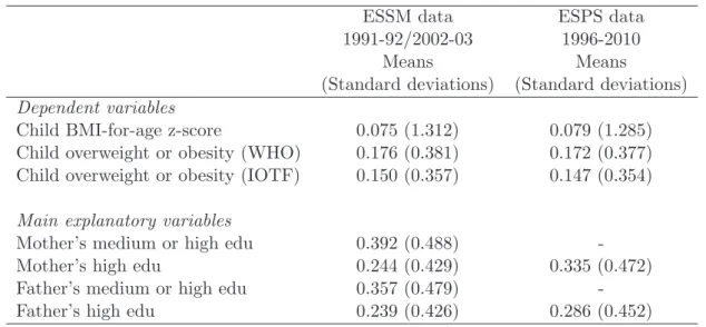
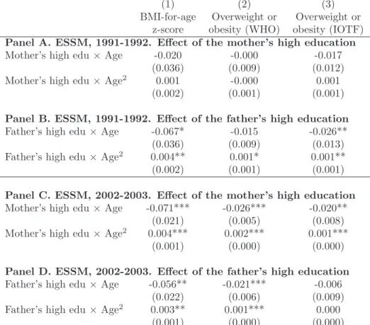
The definitions and summary statistics of the variables of interest are given in Table 1. In the ESSM sample, 17.6% of children are overweight or obese according to the WHO standards and 15.0% according to the IOTF reference. That the prevalence is higher according to the WHO definition than to the IOTF definition has already been found in the previous literature (Gonzalez-Casanova et al., 2013; Rangelova et al., 2014). Note that mean BMI-for-age z-scores and overweight or obesity prevalence are similar across surveys, which suggests that reported height and weight are reliable in the sense that they are stable. The distributions of the education variables in the ESSM and ESPS are somewhat different, because the education variables are not defined in the same way due to data limitations.
[Insert Table 1 here]
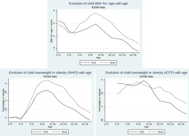
Figure 1 displays the BMI-for-age z-score and the overweight or obesity status as a function of age, separately for boys and girls, in the ESSM data. For the z-score and for overweight or obesity status according to WHO standards, we use the following age groups: 0-2, 1-3, ..., 15-17. For overweight and obesity status according to the IOTF standards, the age groups go from 2-4 to 15-17, since overweight is not defined for children less than 2 in this approach. A non-linear pattern is found for all (proportional) body weight measures for both genders. BMI-for-age and overweight increase or remain stable between birth (or
age 2) and age 8, and decrease afterward. Between ages 2 and 8, the increase in BMI-for-age and overweight status (WHO) seems to be faster for boys than for girls. In contrast, there is some evidence of a decrease in BMI-for-age and overweight (WHO and IOTF) after age 8 for boys and girls. Moreover, in our data, the decrease is greater for girls than for boys. Additional descriptive statistics show a decline in overweight prevalence from 21.3% at ages 8 to 6.3% at age 17, using the two waves of the ESSM.
We also find a decrease in overweight prevalence from 20.2% at ages 7-9 (in 2002-2003) to 8.7% at ages 14-15 (in 2002-2003), for girls, using one single wave of the ESSM.12
We observe a steep decline in overweight for girls in the ESPS as well, from 19.4% (in 2002-2004) and 18.3% (in 2006-2008) at ages 7-9, to 11.1% (in 2002-2002-2004) at ages 14-15.13
The overweight prevalence at ages 14-15 is greater in the ESPS; given that the sample size is larger in the ESPS than in the ESSM, the descriptive statistics from the ESPS might be more reliable here. In any case, since we observe the same pattern in both the ESSM and ESPS, we believe that the sharp decrease in overweight with age for girls is not statistical noise.
This steep decline in reported proportional body weight for girls goes hand in hand with a decrease in measured proportional body weight, but this decrease in smaller: using measured data, it has been shown that approximately 19.5% of girls (in 2007) are over-weight or obese at ages 7-9, versus 16.0% (in 2003-2004) at ages 14-15 (DREES, 2011). Thus for girls ages 7-9, overweight prevalence in the ESSM and ESPS is consistent with the prevalence from DREES (2011). But for girls ages 14-15, the prevalence is much smaller in the ESSM and ESPS than in DREES (2011). This gap is due to difference in the type of data: reported data (in the ESSM and ESPS) capture body weight perceptions, while measured data (in DREES) reflect actual body weight. Reported data are relevant be-cause perceptions likely determine weight-related control behaviors – in other words, one cannot expect an individual who does not perceive he is overweight to be careful with his weight.14
[Insert Figure 1 here]
12Here we use the survey year that is the nearest to the survey years from DREES (2011), for comparison
purposes.
13
We chose the survey years to match those of the ESSM and of DREES (2011), for comparison purposes.
14
Our model (1) is estimated separately by age groups, so it perfectly controls for any change in unob-served variables with are correlated with age. We estimate this model using our reported body weight data and find that the gradient in education is U-shaped with age. Our descriptive statistics highlight that the gap between reported and measured body weight is a function of age. If that gap depends only on age, then our findings imply that the gradient in education and measured body weight is U-shaped.
Figure 2 shows age-related changes in BMI-for-age and overweight, separately by parental educational level, in the ESSM data. Both maternal and paternal education levels are negatively associated with child body weight: children whose parents have a high education have a lower BMI-for-age and are less likely to be overweight than those whose parents have a low or medium education.
Overall, between ages 2 and 8, proportional body weight generally increases or re-mains stable for both children whose parents have a low or medium educational level and children whose parents have a high educational level. After age 8, proportional body weight decreases. We find some evidence that before age 8, the speed of the increase in (proportional) body weight is greater for children whose parents have a low and medium education. Moreover, after age 8, the decrease in body weight is sharp for children whose parents have a low or medium level of education, whereas it is at most slow for children whose parents have a high level of education. As a result, the gap between the two curves first increases and then decreases with age, which suggests that there is process of diver-gence in body weight among children before age 8, followed by a process of converdiver-gence afterward.
In the bottom left subfigure, the probability of overweight (IOTF) for children whose mother has a low or medium level of education follows the same pattern: it first increases and then decreases with age. But the trajectory of overweight for children whose mother has a high level of education is different, since the probability of overweight continuously decreases with age. In spite of this difference, the gap between children also strengthens before age 8 and weakens afterward in this subfigure.
[Insert Figure 2 here]
3.4 Methods
To describe the evolution of the gradient across childhood and adolescence in a precise manner, we use the following model, that we estimate separately for different age groups:
BC = α + SESPβ+ DAC + XC,Pχ+ v (1)
where BC denotes a child body weight outcome, SESP the SES variable (i.e. parental
education or family income), DAC a series of dummy variables for the child age, and XC,P child- and parents-level control variables. The coefficient of interest is β which indicates
whether the gradient in SES and child body weight is positive and significant. The model is estimated separately for children ages 0-2, 1-3, 2-4, ... and 15-17. Note that these age groups overlap, in order to smooth our estimates of the gradient.
Like Figure 2 in the descriptive statistics, this multivariate model will highlight that the association between SES and child body weight outcomes has a U-shape across childhood. To describe this non-monotonic evolution of the gradient, we use the following model for the total sample of children:
BC = α + SESPβ+ ACδ1+ A2Cδ2+ [SESP × AC]φ1+ [SESP × A2C]φ2+ XC,Pχ+ v (2)
where AC and A2C denote the child age and age squared; SESP × AC is an interaction
term between SES and child age; and SESP × A2C denotes the interaction between SES
and child age square. If φ1 is negative and significant and φ2 is positive and significant,
then the inverted U-shape of the gradient is statistically significant.
When estimating equation (2), we generally include the control variables, without interacting them with child age and age square. We thus assume that the impact of the controls is stable with age. In some analyses, we relax this assumption and allow the impact of the controls to change with age. Specifically, we estimate a fully interacted model in which the controls are all interacted with age and age square.
Equation (2) is flexible enough to allow the relationship between body weight and age to be different for low- and high-SES children. Indeed, equation (2) can be rewritten as:
BC = α + SESP[β + ACφ1+ A 2
Cφ2] + [ACδ1+ A 2
Cδ2] + XC,Pχ+ v (3)
For low-SES children (for instance, parental education is low, i.e. SESP = 0), the
association between body weight and age is captured by BSESP=0
C = α + [ACδ1+ A2Cδ2] +
XC,Pχ+ v. In contrast, for high-SES children (SESP = 1), the association between body
weight and age is different and is captured by BSESP=1
C = α + [β + AC(φ1+ δ1) + A2C(φ2+
δ2)] + XC,Pχ+ v.
Note that the model does not assume that both children for whom SESP = 0 and for
whom SESP = 1 have a peak in body weight during childhood. It does not assume either
that when there is a peak for both children for whom SESP = 0 and for whom SESP = 1,
peak will be at age −δ1
δ2,
15
and there will be no peak if δ1 = 0. For children for whom
SESP = 1, the peak will be at age −φ1 +δ1
φ2+δ2,
16 and there will be no peak if if φ
1+ δ1= 0.
The models are estimated using OLS. When the child body weight outcome is a dummy variable, the model is then a linear probability model (LPM). Although in this case we could have used a logit or a probit model, we prefer to use a LPM because standard sta-tistical software do not estimate the real magnitude of the interaction effects in nonlinear models, especially when they are several interaction terms like in our models (Ai and Nor-ton, 2003) and coefficients are easier to interpret in LPMs . We calculate robust standard errors.
4
Results
4.1 Main results
To accurately depict the evolution of the gradient in body weight and SES across child-hood, we start by estimating equation (1) separately for children ages 0-2, 1-3, 2-4, ... 15-17, using the ESSM data. We alternatively use child BMI-for-age and overweight or obesity status as our dependent variables. Our main explanatory variables are either the dummy for whether the mother has a high educational level or the dummy for whether the father has a high educational level. In Figure 3, we graph the βs coefficients on the parents’ education as a function of child age group.
For the top left subfigure, the sample contains children who live in the same house-hold as their mother (i.e. children who live with their mother and father, or only with their mother), the dependent variable is the child BMI-for-age, and the main explana-tory variable is the mother’s high education. The dots represent the β coefficients on the mother’s high education, whereas the bars capture the confidence intervals. For any age group, the correlation between the mother’s education and the child BMI is negative and significant. In addition, the association follows a U-shape with child age: the correlation between the mother’s education and child BMI first strengthens (in absolute values) be-tween birth and age 5 approximately, and then weakens from age 5 to 17. This implies that social differences in (reported) body weight first increase in early childhood and then decrease at the end of childhood and during adolescence. The left subfigure on the second
15
The algebra is: ∂B
SESP =0 C
∂AC = 0 ⇔ AC= − δ1 δ2. 16The algebra is: ∂BCSESP =1
∂AC = 0 ⇔ AC= − φ1+δ1 φ2+δ2.
row presents the gradient in the mother’s high education and child overweight or obesity status using the WHO reference. Again, the association is negative and significant for all age groups, which implies that there are social inequalities during all childhood years. The gradient follows a (an inverted) U-pattern, meaning that social inequalities increase and then decrease over childhood. These results are consistent with those found when the dependent variable is child BMI. Finally, the bottom left subfigure shows that at any age the mother’s education is negatively and significantly associated with the probability that the child is overweight or obese according to the IOTF standards. Consistent with the previous findings, the association follows a U-shape.
Previous research on child inequalities in childhood has mainly focused on the impact of the mother’s education on child health, leaving the father’s education aside. One of our contributions here is to explore the effect of the father’s education. The right hand side subfigures in Figure 3 show our results. The findings are very similar to those obtained for maternal education. A significant association between the father’s education and the child BMI and overweight or obesity is found for most age groups. Moreover, the gradient follows an inverted U-pattern for our three outcomes.
[Insert Figure 3 here]
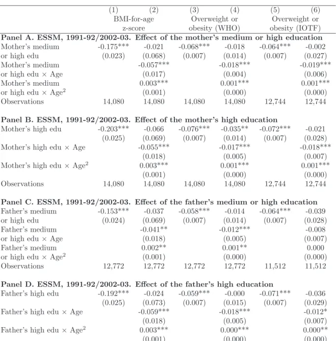
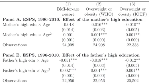
The results presented so far are based on separate estimations of equation (1) by child age groups, and suggest that the gradient reinforces and then weakens with age. To go one step further, we specify this functional relationship between parents’ education and child outcomes, in equation (2). This model is estimated using a sample of children of all ages from the ESSM data and the findings are presented in Table 2. In the four panels, we use alternative parents’ education variables. In columns (1) and (2), the dependent variable is the child BMI-for-age; in columns (3)-(4), the overweight or obesity status according to the WHO definition; and in columns (5)-(6), the overweight or obesity status using the IOTF reference. Columns (2), (4), and (6) present the estimates of equation (2).
In panels A and B, we focus on the impact of the mother’s education, and the sample contains children who live in the same household as their mother. Panel A, column (1), presents the slope of the gradient in the mother’s high/medium education and child BMI-for-age. The correlation is negative and significant. The model in column (2) adds the interaction terms between the mother’s medium or high education and child age and age square. The coefficient on the mother’s education now gives the relationship between
education and BMI for children aged 0. This coefficient is not significant, which means that the slope of the gradient is not significant for children aged 0. The interaction term between education and age is negative and significant, whereas that between education and age square is positive and significant. This implies that the gradient has an inverted U-shape, and that social inequalities in reported BMI rise and then decline across childhood. The gradient is the largest around age 9.17 Columns (3) and (5) suggest that the mother’s
medium or high education is correlated with a 6.4-6.8 percentage points significant decrease in the probability that the child is overweight or obese. Consistent with the results in column (2), the interaction terms in columns (4) and (6) reveal that social inequalities in reported overweight first widen and then narrow during childhood.
In panel B, the main explanatory variable is a dummy for whether the mother has high education, rather than medium or high education. The results are qualitatively similar to those in panel A. The association between the mother’s education and child BMI and overweight is negative and significant. The interaction terms in columns (2), (4), and (6) indicate that the association follows a U-shape over childhood. For instance, maternal high education is correlated with a 5.30 percentage points decrease in child overweight or obesity (IOTF) at age 2, but a 9.62 percentage points decrease at age 8, and a 1.25 percentage point decrease at age 17.18
The gradients in child BMI and overweight reach their peak around the age of 8.
Panels C and D show that the father’s education is also negatively and significantly correlated with the child BMI and overweight. The size of the gradient in the father’s education is either similar or slightly smaller than the gradient in the mother’s education. Like for maternal education, the gradient in paternal education generally follows a signif-icant inverted U-shape with child age. For instance, paternal high education is correlated with a 5.87 percentage points decrease in child overweight or obesity (IOTF) at age 2, but a 9.11 percentage points decrease at age 8, and a 4.52 percentage points decrease at age 17.19
[Insert Table 2 here] 17
We use estimates with four decimals, rather than just three like in the table. The second derivative with respect to education and to age equals zero around age 9. The algebra is the following: −0.0571 + 2 × 0.0033 × Age = 0 for Age = 8.65.
18
Using the estimates with four decimals, the size of the gradient in maternal high education and child overweight or obesity at each age equals −0.0210 − 0.0182 × Age + 0.0011 × Age2.
19
The size of the gradient in paternal high education and child overweight or obesity at each age equals −0.0367 − 0.0124 × Age + 0.0007 × Age2.
4.2 Robustness analysis
4.2.1 Additional control variables and the income gradient
We here investigate whether our result on the trajectory of the education gradient is robust to the inclusion of additional controls – family income and interaction terms between income and age polynomials in particular. By doing so, we also examine the trajectory of the income gradient in childhood.
First, we include three additional explanatory variables in our model, namely family income, maternal labor market status, and parental body weight. Indeed, parents’ edu-cation may be a proxy for other SES variables, such as family income or parents’ labor market status. To isolate the effect of parents’ education, we thus need to re-estimate our model controlling for these variables. Moreover, parents’ body weight may be an omitted variable in our model if it has an impact on both parents’ education and child body weight. In particular, the recent literature provides evidence on the intergenerational transmission of body weight (Classen, 2010; Classen and Hokayem, 2005; Monheit et al., 2009, for the US; Costa-Font and Gil, 2012, for Spain).
In the ESSM, income is defined as monthly pre-tax family income. In the 1991-1992 wave of the data, income is given in ten brackets, and we thus compute the middle of the brackets. Consequently there is some measurement error in the income variable. In the 2002-2003, the exact income level is available. Using the consumer price index, we adjust income so that the variable is comparable across waves. In our specification, we take the logarithm of income to account for the non-linearity in the relationship between income and body weight.
We measure maternal labor market status using a dummy for whether the mother participates actively in the labor market (i.e. she is employed or unemployed). Parental body weight indicators are parents’ BMI and dummy variables for whether the parents are overweight or obese.
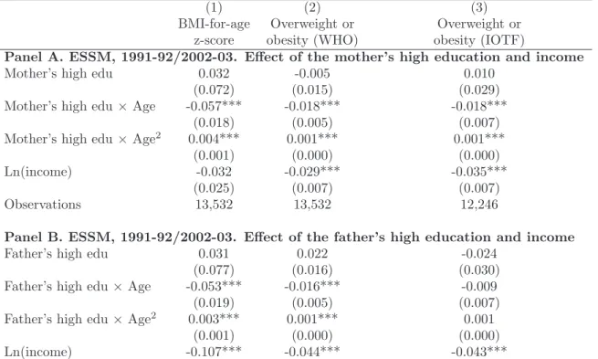
Our findings are presented in Table 3. The models control for child age and age square, the basic controls, and income. In addition, regressions in panels A control for the mother’s education, the mother’s labor market status, and the mother’s body weight, whereas regressions in panel B control for the father’s education and the father’s body weight. In most specifications, the coefficients on the interaction terms remain highly significant, which implies that our main results on the education gradient are robust to
the inclusion of additional controls. Moreover, the coefficients on income are negative and generally significant, suggesting that income plays a protective role against overweight. For instance, in panel A, column (2), when the logarithm of income increases by 1 (i.e. when income is multiplied by 2.7), the probability that the child is overweight (WHO) decreases by 2.9 percentage points.20
[Insert Table 3 here]
We now test whether our results on the trajectory of the education gradient are affected by the inclusion of interaction terms between income and age polynomials, and investigate the shape of the gradient in income at the same time. We start by estimating equation (1) using the logarithm of income as our SES variable, separately by age groups. Here we do not control for parents’ education. The results, which are presented in Figure 4, show that for most age group family income is negatively and significantly associated with body weight. Moreover, the gradient in income has an inverted U-shape across childhood.
[Insert Figure 4 here]
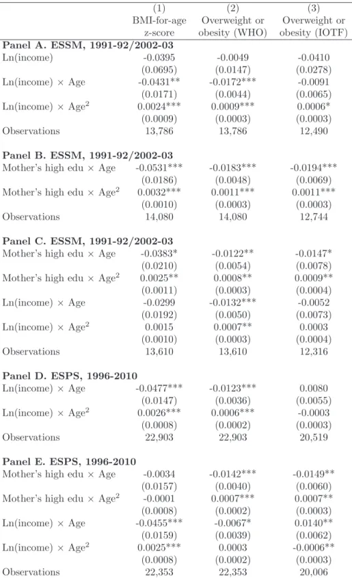
We then estimate equation (2), still using income as our SES proxy, for the sample of children of all ages. We first include the basic controls, not interacted with age and age square. The results (available upon request) show that the interaction terms between income and age and age square are not significant, whether we control for parents’ edu-cation or not. However, this model assumes that the effect of the control variables does not depend on child age. Given that interaction terms between the control variables and age could play the role of third common hidden factors in the equation, omitting these variables from our model may bias our estimates on interaction terms between income and age. We thus estimate a fully interacted model (that relies on weaker assumptions), in which all the control variables are interacted with age and age square. The results are shown in Table 4.
In panel A, we do not control for parental education. In both columns (1) and (2), the gradient in income has a significant inverted U-shape. Column (1) implies that the correlation between income and BMI-for-age is the strongest in absolute values at age 9.
20
The results also show that maternal labor market status is not significantly associated with child body weight and that parents’ body weight is positively and significantly correlated with child body weight. We also estimate models that control for parents’ general health, using the 2004-2010 ESPS data. The results are consistent with an inverted U-shape gradient in education.
In column (3), the signs of the coefficients are consistent with the U-shape trajectory, but one of the interaction terms is not significant.21
In panel B, we estimate the fully interacted model using the mother’s high education as our SES variable. We show the coefficients on the interaction terms, but not that on the mother’s education, for space reasons. The shape of the education gradient clearly emerges. Moreover, the coefficients on the interaction terms have the same magnitude as in the model in Table 2, panel B (in which the controls are not interacted). Thus for education, the results of the specification in which we do not interact the controls are similar to those from the fully interacted model – for this reason, in Tables 5-9 in which we will only focus on education, we won’t interact the control variables.
In Table 4, panel C, family SES is measured using both education and income. In columns (1) and (3), the interaction terms for income are no longer significant. In con-trast, in column (2), the evolution of the income gradient with age remains significant. Interestingly, this panel highlights that the trajectory of the education gradient is robust to the inclusion of interaction terms for income.
Finally, in panels D and E, we re-do our analysis using the ESPS data. Panel D corroborates the findings on the trajectory of the income gradient from panel A. In panel E, we add the mother’s high education. Column (1) still shows an (inverted) U-shape for the income gradient. In column (2), the results on income are less clear. In column (3), the interaction terms on income switch signs. This surprising result is due to multicollinearity (i.e. the high level of correlation between income and education in this specific model, in other words we “overcontrol” for family SES here), and does not mean that inequalities in income and overweight (IOTF) decrease and then increase in childhood.
Table 4 thus provides some evidence that the gradient in income has the same shape as the gradient in education. However, the results on the education gradient are clearer and more robust, maybe because there is less measurement error in education than in income. For this reason (and for space reasons), the rest of the paper only investigates the role of education.
[Insert Table 4 here] 21
We find that the difference in our results (between the model in which the controls are not interacted and the fully interacted model) is mainly due to the inclusion of the interaction terms between survey year dummies and age and age square. Indeed, there is a correlation between year dummies and income on the one hand, and year dummies and body weight on the other hand. The correlation between year dummies and income may be due to the change in the income variable over time (in 1991-1992, income is given in brackets, whereas in 2002-2003, we have information on the exact family income level).
4.2.2 Cohort fixed effects
The variation in the education gradient with age that we show above will not quantify the evolution of social inequalities in health over the life cycle in the presence of cohort effects. A natural strategy is then to include cohort fixed effects in the model. We assume that all children born in a 5-year interval belong to the same cohort. If we were to control for cohort fixed characteristics in our model when we use the ESSM data, they would be very highly correlated with child age and with the survey year fixed effects, because the ESSM survey is only carried out every ten years (1991-1992 and 2002-2003). Consequently, we would face a multicollinearity problem.
In contrast, it is possible to include cohort fixed effects in our model when we use the ESPS data, because this survey is done every one or two years. We create a series of cohort dummies for children born before 1984, between 1985 and 1989, between 1990 and 1994, ... and between 2005 and 2010, and re-run our model including these cohort dummies. The standard list of controls is also included. The results, which are reported in Table 5, show that the gradients in the mother’s education and child overweight or obesity, in the father’s education and child BMI, and in the father’s education and child overweight or obesity still take the form of an inverted U-shape.
[Insert Table 5 here]
To explore more in depth the role of cohorts’ characteristics, we compare the effect of parental education on child body weight when we control for cohort fixed effects and when we do not. We focus on the impact of the mother’s high education and child BMI-for-age, for space reasons. We represent the effect as a function of age in Figure 5.22
The figure underlines that accounting for cohort fixed effects only has a small influence on the trajectory.
[Insert Figure 5 here] 22
To get the curve for the model “not accounting for cohort fixed effects,” we proceed as follows: we estimate equation (2) not including cohort fixed effects; using the estimated coefficients ˆβ, ˆφ1, and ˆφ2, we
compute the effect EF of the mother’s education, which is the difference in body weight between children whose mother has a high level of education (SESP = 1) and children whose mother has a low level of
education (SESP = 0), which writes EF = ˆBSESP =1
C − ˆB
SESP=0
C = ˆβ+ ACφˆ1+ A2Cφˆ2; finally we graph
the curve representing the effect EF as a function of age. To get the curve for the model “accounting for cohort fixed effects,” we follow the same steps but include the cohort fixed effects when we estimate equation (2). The curves in Figure 5 are below zero because of the negative correlation between parents’ education and child BMI-for-age.
4.2.3 Child fixed effects
Our main results could also be biased because we do not account for child fixed char-acteristics. To test the robustness of our findings, we re-estimate our model using the ESPS data and including child fixed effects (which capture race or ethnicity for instance). In that setting, the interaction terms between education and child age are still identified because child age varies over time. The number of observations that we use is smaller than in our main specification, because only a fraction of children are followed over time. In particular, the observations from the 2010 wave are dropped due to the fact that the ESPS sample was completely renewed in 2010. The results, which are presented in Table 6, are consistent with the (inverted) U-shape of the gradient.
[Insert Table 6 here]
4.2.4 Other robustness tests
Our BMI z-scores are derived from the WHO Growth Charts. However, our results on the (inverted) U-shape of the gradient seem to be robust to the use of alternate growth references. Indeed, when we use z-scores derived from the British 1990 Growth Charts or the 2000 CDC Growth Charts, the gradient either slightly strengthens or remains stable from birth to age 8, and clearly weakens after age 8.
So far, our models have accounted for either the mother’s education or the father’s education. We also estimate models in which we control for both maternal and paternal education and all interaction terms. The results are consistent with the (inverted) U-shape of the gradient. However, these results are not as clear as when we control for either maternal or paternal education, since the interaction terms are smaller and some of them lose their significance. The reason is that maternal and paternal education are correlated, due to assortative mating in particular. It seems to us that maternal and paternal education are too correlated to be included in the same model.
Note also that when we estimate the evolution of inequalities using our equation (2) but controlling for child age dummies instead of child age and age squared, the results are almost unaffected.
Moreover, there is no evidence that the U-shape is due to a change from parents’ reported height and weight to child reported height and weight. Indeed, when in the ESPS data we only keep children whose body measures are reported by their parents, the
U-shape still clearly appears.
Finally, we also re-estimate our models dropping children ages 0-2. Indeed, evaluating overweight/obesity at ages 0-2 is touchy. Clinicians disagree on whether there can be an overweight problem in infancy. In addition, overweight in infancy is poorly defined – the literature and clinical guidelines use different criteria to define overweight in early childhood (Heinzer, 2005). The results, which are presented in Table 7, are consistent with our previous findings: the interaction terms always have the expected sign, the two interaction terms are significant in all the models for the mother’s education (panel A, columns (2), (4) and (6)) and in one model for the father’s education (panel B, column (4)).
We now compare Table 7 with Table 2, for which very young children were included in the sample. For the mother’s high education, the significance level is 1% or 5% in Table 7, whereas it was always 1% in Table 2, and the magnitude of the interaction terms is either similar or slightly larger in absolute value. For the father’s high education, the interaction terms are no longer significant in column (2), there is only one significant interaction term in column (6) – the loss of significance could be due to the decrease in the sample size – and the coefficients are slightly greater in absolute value in column (4).
[Insert Table 7 here]
4.3 Additional results
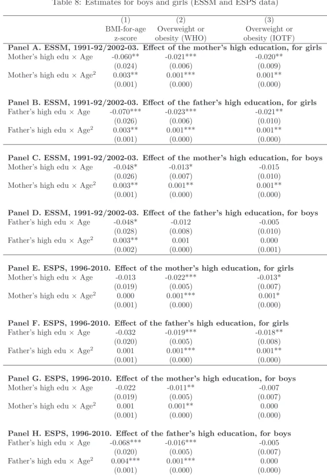
4.3.1 Analysis by gender
We now relax the assumption that there is the same evolution of the gradient with age for boys and girls. This analysis is motivated by previous studies for the US highlighting that the evolution of the gradient with age is different between genders (Wang and Zhang, 2006). To this end, we re-estimate our model separately for boys and girls and show our estimates in Table 8. The results are in line with our previous results. Indeed, the signs on the interaction terms are consistent with an inverted U-shaped gradient in all models. In addition, the coefficients are significant in a number of models. Interestingly, the relationship between parents’ education and child body weight is not sex-specific, since we find it for mothers-daughters and fathers-sons, but also for mothers-sons and fathers-daughters.
4.3.2 Analysis by survey year
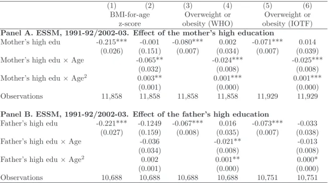
We also re-estimate our model separately for 1991-1992 and 2002-2003, in the ESSM, and for 1996-2004 and 2006-1010, in the ESPS, to see whether the shape has emerged over time. Note that when we use the ESPS, we include several survey years to avoid small samples. The results are presented in Table 9. In all panels, the signs on the interaction terms are consistent with a U-shape. The U-shape can be observed as of 1991-1992, and in each subsequent period.
[Insert Table 9 here]
5
Discussion
Using two datasets containing approximately 40,000 children observations, we investigate the relationship between parental education and child reported body weight across child-hood in France. Reported data capture body weight perceptions, which likely have an influence on weight-related behaviors on their own. Our findings indicate that children whose parents have a high level of education have a lower BMI-for-age and are less likely to be overweight (Table 2). Our results for French children echo findings for French adults, which are also based on reported height and weight data. Specifically, De Saint Pol (2009a) highlights significant differences in BMI depending on occupation, standard of living, and educational level, for both females and males, in 2003. Moreover, Etil´e (2014) uses the recentered influence function technique to quantify the role of education in BMI and finds that educational expansion decreased BMI inequalities between 1981 and 2003. Finally, Singh-Manoux et al. (2010) highlight that inequalities in socioeconomic status (measured by education or income) and height have remained significant and stable between 1970 and 2003.
The evolution of reported (proportional) body weight across childhood is non-monotonic in our data. BMI-for-age and overweight status generally increase between ages 2 and 8 and decrease afterward (Figure 1). The increase in early childhood is consistent with the adiposity rebound, which refers to the increase in BMI that starts (after a nadir) between ages 3 and 8 in most countries. Note however that the adiposity rebound is assessed using the unadjusted BMI (computed using measured height and weight) and body composi-tion measures in the medical literature, and not BMI-for-age z-scores or overweight status (computed using reported data). In our data, additional results show that the rebound
in unadjusted BMI happens between ages 4 and 6. Moreover, we show a sharp decrease in overweight after age 8 for girls. This pattern is found in our two datasets, which sug-gest that it is not due to statistical noise. In general, the whole trajectory of reported body weight across childhood in our analysis is in line with international findings: for instance, Costa-Font and Gil (2012) also use reported height and weight and find a peak in overweight in childhood in Spain.
In the absence of any control variable, our data already suggest that the gradient follows an inverted U-shape with age. Specifically, when we distinguish the trajectory of body weight according to parental education, we observe that between ages 2 and 8 the speed of the increase in body weight is greater for children whose parents have a low and medium education than for children whose parents have a high educational level, and that later on, the speed of the decrease in body weight is also larger for children whose parents have a low or medium educational level (Figure 2). These differences in the trajectory of body weight with age between children imply that the correlation between family SES and child body weight strengthens in early childhood and then weakens for older children. The econometric specification, that includes control variables, support this finding. The gradient in parents’ education and child body weight has an inverted U-shape across childhood, which implies that the gradient first widens and then narrows as children get older. They reach their peak at the age of 8. This result holds when we estimate our models separately by age group and when we use the full sample of children of all ages. This results is also found when we account for maternal labor market status, family income, parental body weight, cohort fixed characteristics, or child fixed traits. Consistent with education, the income gradient is also U-shaped across childhood, although our results may be less robust.
Our findings on the trajectories of the education and income gradients in child body weight in France are somewhat different from related results from the literature. Indeed, Murasko (2013) finds a strengthening of the gradient in family income and child (measured) BMI in the US. Howe et al. (2013) show that the gradient in maternal education and offspring fat mass increases with age for girls, and remains stable for boys, in the UK. Moreover, the gradient in family income and child health becomes more pronounced as children get older in France, which implies that the health of children from families with low income erodes faster with age (Apouey and Geoffard, 2014). In addition, recent research shows a stability of the gradient in general health in the UK (Apouey and Geoffard, 2013;
Howe et al., 2013), although this is still a debated conclusion (Currie et al., 2007; Case et al., 2008; Propper et al., 2007). Taken together, these findings highlight that the trajectory of the gradient in childhood depends on the country and on the child outcome of interest (reported or measured anthropometric outcomes, general health, etc).
A possible explanation for the inverted U-shape of the gradient emphasizes the role of socialization and schooling in youth, echoing the theory of West (1988, 1997). This author focuses on the UK and argues that social health inequalities are strong in childhood, that they decrease or virtually disappear in youth (starting age 12 in his approach), and re-emerge in late youth. The empirical results of West have been recently discussed, as several authors did not find any weakening of health inequalities during adolescence in the UK (Apouey and Geoffard, 2013; Case et al., 2008). However, West’s intuition on the role of socialization remains relevant in our context to explain the decrease in the education gradient after age 8 (note that in West’s approach, inequalities start decreasing later, around age 12). For West, one of the causes of the decrease in youth is that adolescents progressively detach themselves from their parents and their parental home, and spend more time at school and with their peers (West, 1988, 1997). In the context of our study, socialization at school may have an influence on weight-related behaviors and body weight perceptions. It is possible that starting age 8 this socialization effect becomes more prominent while the effect of parents’ education starts decreasing. Consistent with this intuition, another strand of literature has shown significant peer effects in primary and secondary schools, related to body weight, body perception, physical activity, and eating habits in Canada and the US (Ali et al., 2011; Fortin et al., 2011; Halliday et al., 2009; Renna et al., 2008; Trogdon et al., 2008). Finally, (mandatory) physical education courses in primary school may also lead to a weakening of the association between parents’ education and body weight.
The inverted U-shape in the gradient in reported body weight may reflect an inverted U-shape in the gradient in measured body weight. In that case, social inequalities in body weight are neither cumulative nor irreversible, since inequalities would start decreasing around age 8. In this approach, a potential explanation of the shape of the gradient has to do with “selective overweight.” Indeed, reported body weight follows an inverted U-shape across childhood for both boys and girls in France (see Figure 1). In parallel, there is some evidence that measured body weight also follows this shape, although the
age of the peak is uncertain and might be around 10-11.23
In age groups in which few children are overweight, before age 4 and after age 14, there may be almost no selection at play: only the most prone to overweight (because of genetic factors, not necessarily related to parental characteristics) will be overweight. In that case, parental education will only play a minor role and the gradient will be small. In contrast, in age groups in which overweight is more prevalent (because child weight is particularly affected by socioeconomic and environmental conditions), parental education will play an important role. Hence, in age groups where overweight is more widespread, a selection process may be at play, which may explain why a stronger gradient is observed. Overall, if there is such a selection process, the equalization of body weight after age 8 will be due to the “natural” decline in BMI and to the decline in selectivity in overweight with respect to parental education.24
Given that reported anthropometric data differ from measured data (there is a so-called “bias” or “reporting style” in reported data), the shape of the education gradient across childhood may also partly capture a change in the association between parents’ education and the reporting style across childhood. More precisely, parents may become worried about social norms regarding body weight around age 8, soon after the child enters primary school. If children whose parents have a low level of education under-report their true body weight starting age 8, then we will observe that the gradient has an inverted U-shape although in reality the gradient increases with age (assuming that children whose parents have a high level of education do not over-report their body weight, which is an acceptable assumption in our opinion).25 In that case, the change in reporting style with
education and age will bias the measurement of the evolution of health disparities. Of particular relevance would thus be research on the evolution of the bias with family SES and age (taken together). As far as we are aware, this topic has not been explored so far. Indeed, the literature that assesses the validity of self-reported body weight in the 23
We did not find data on the evolution of the BMI-for-age z-score with age in France. A report based on measured data shows that for girls overweight prevalence remains constant or slightly increases between ages 7-9 and 10-11, and then clearly decreases between ages 10-11 and 14-15. The peak is then at ages 10-11. For boys, overweight prevalence increases between ages 7-9 and 10-11, and then decreases between ages 10-11 and 14-15. The peak is also at ages 10-11 (DREES, 2011). However, these measured data on overweight by age are not precise, since they are only calculated for some specific age groups (ages 5-6, 7-9, 10-11 and 14-15), and not at each age. Consequently, there is some uncertainty about the exact age of the peak, which might in reality be before age 10.
24
We are thankful to a referee for suggesting this explanation.
25
Computing the extent of the bias that would change the U-shaped trajectory into an increasing tra-jectory is difficult. It would be possible only if information on the coefficients of the model that regresses measured body weight on child age, parents’ education, their interaction terms, and the control variables was available.