HAL Id: hal-00304647
https://hal.archives-ouvertes.fr/hal-00304647
Submitted on 1 Jan 2002HAL is a multi-disciplinary open access archive for the deposit and dissemination of sci-entific research documents, whether they are pub-lished or not. The documents may come from teaching and research institutions in France or abroad, or from public or private research centers.
L’archive ouverte pluridisciplinaire HAL, est destinée au dépôt et à la diffusion de documents scientifiques de niveau recherche, publiés ou non, émanant des établissements d’enseignement et de recherche français ou étrangers, des laboratoires publics ou privés.
in rainfall-runoff models illustrated using the PDM
R. J. Moore, V. A. Bell
To cite this version:
R. J. Moore, V. A. Bell. Incorporation of groundwater losses and well level data in rainfall-runoff models illustrated using the PDM. Hydrology and Earth System Sciences Discussions, European Geo-sciences Union, 2002, 6 (1), pp.25-38. �hal-00304647�
Incorporation of groundwater losses and well level data in
rainfall-runoff models illustrated using the PDM
R.J. Moore and V.A. Bell
Centre for Ecology and Hydrology, Wallingford, Oxon, OX10 8BB, UK
Email for corresponding author: [email protected]
Abstract
Intermittent streamflow is a common occurrence in permeable catchments, especially where there are pumped abstractions to water supply. Many rainfall-runoff models are not formulated so as to represent ephemeral streamflow behaviour or to allow for the possibility of negative recharge arising from groundwater pumping. A groundwater model component is formulated here for use in extending existing rainfall-runoff models to accommodate such ephemeral behaviour. Solutions to the Horton-Izzard equation resulting from the conceptual model of groundwater storage are adapted and the form of nonlinear storage extended to accommodate negative inputs, water storage below which outflow ceases, and losses to external springs and underflows below the gauged catchment outlet. The groundwater model component is demonstrated through using it as an extension of the PDM rainfall-runoff model. It is applied to the River Lavant, a catchment in Southern England on the English Chalk, where it successfully simulates the ephemeral streamflow behaviour and flood response together with well level variations.
Keywords: groundwater, rainfall-runoff model, ephemeral stream, well level, spring, abstraction
Introduction
Ephemeral rivers pose special problems for rainfall-runoff modelling. A water balance needs to be maintained over periods when flow ceases in order to simulate correctly the time at which flow restarts. The water balance of catchments where groundwater influences dominate is often affected by the artificial influence of pumped abstractions. Also the lack of a water balance closure within the surface catchment, due to subsurface transfers of water across the catchment boundary, requires special consideration. External spring flow and underflow beneath the gauging station can be important influences.
The purpose here is to develop a generic model component for representing groundwater storage under the influence of pumped abstractions, spring flows and underflows. This model component can be used as part of the configuration of a rainfall-runoff model for application to groundwater dominated catchments. Application of the model component is illustrated here by using it to create an extended form of the PDM rainfall-runoff model, widely used in the UK for flow forecasting (Moore, 1999; Institute of Hydrology, 1992, 1996; CEH, 2000). By way of background, the first part of
the paper reviews the basic form of the PDM model. It then focuses on the PDM’s nonlinear storage representation of an aquifer and how this can be extended to represent ephemeral flows at times when recharge fails to offset “groundwater losses”, particularly those associated with pumped abstractions.
Application of the extended PDM rainfall-runoff model is demonstrated using the Lavant catchment situated on the Chalk of southern England. At times of high groundwater levels, this catchment can become highly responsive to rainfall causing flooding of the town of Chichester. It is demonstrated how both the long-term seasonal response and the dynamic storm response of the catchment are captured by the model when used to simulate both flows and groundwater levels.
The Probability Distributed Model
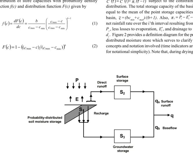
The Probability Distributed Model, or PDM, is a fairly general conceptual rainfall-runoff model which transforms rainfall and evaporation data to flow at the catchment outlet (Moore, 1985, 1986, 1999). Figure 1 illustrates the general
form of the model. The PDM has been designed more as a toolkit of model components than as a fixed model construct and extending a component, as done here to represent ephemeral flows, can be relatively straightforward. Several options are available in the overall model formulation which allows a broad range of hydrological behaviours to be represented.
Runoff production at a point in the catchment is controlled by the absorption capacity encompassing canopy interception, surface detention and soil water storage processes. This can be conceptualised as a simple store with a given storage capacity. By considering that different points in a catchment have differing storage capacities and that the spatial variation of capacity can be described by a probability distribution, it is possible to formulate a simple runoff production model which integrates the point runoffs to yield the catchment direct runoff prior to translation to the catchment outlet as surface runoff (Moore, 1985). Other models utilising this probability distributed principle include the Xinanjiang model (Zhao et al., 1980) and Arno model (Todini, 1996).
The standard form of PDM employs a truncated Pareto distribution of store capacities with probability density function f(c) and distribution function F(c) given by
(1)
(2)
such that cmin≤ c ≤ cmax. Here the shape parameter b controls the form of variation between the minimum capacity, cmin, and the maximum capacity, cmax. Over the i’th time interval
(t, t+∆t) with net rainfall rate πi, the volume of basin direct runoff per unit area generated from this distribution of stores is
(
t t)
t (S(t t) S(t))V +∆ =πi∆ − +∆ − (3)
where the total water in store across the basin, expressed as a depth over the basin, is given by
( )
{
(
)
1}
min max * max min min ( )1 ( ()) ( ) + − − − − + =c c c c C t c c b t S (4)with a maximum value Smax when C*(t) = c
max. Here, C*(t) is
the critical store capacity below which all stores are saturated at time t and generating runoff. This capacity is uniquely related to the water in store across the basin, S(t), such that (5) and evolves over the interval according to
( )
C( )
t +( )
tC*τ = * πi τ− subject to the constraints of the
distribution. The total storage capacity of the basin, Smax, is equal to the mean of the point storage capacities over the basin, c =(bcmin+cmax)/(b+1). Also, πi=Pi−Ei′−di is the
net rainfall rate over the i’th interval resulting from rainfall,
Pi, less losses to evaporation, Ei′, and drainage to recharge,
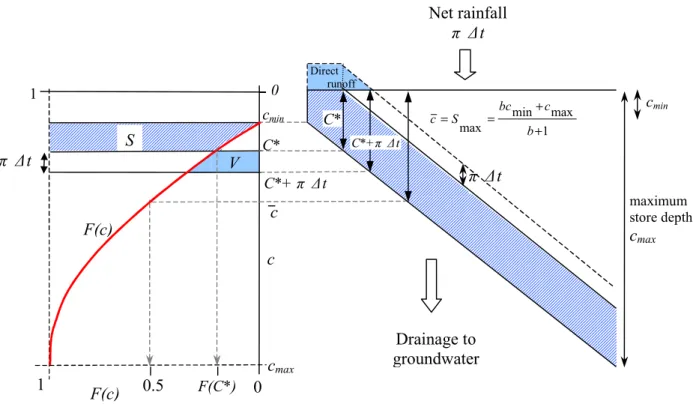
di. Figure 2 provides a definition diagram for the probability distributed moisture store which serves to clarify the main concepts and notation involved (time indicators are omitted for notational simplicity). Note that, during drying, water is
( )
( )
c c c c c c b dc c dF c f b max min max 1 max min − − − = = −Fig. 1. The PDM rainfall-runoff model
c c cmin≤ ≤ max
( )
c(
c c c c)
F b min max max ) ( ) ( 1− − − =( )
{
(
)
1/( )1}
min max min max min ( )1 ( ()) ( ) * + − − − − + =c c c S S t c c b t Cassumed to distribute freely between stores of different depth so as to maintain an equal water depth across stores that are not full (Moore, 1985).
Water is lost as evaporation at a rate Ei′ from the water in
store as a function of the potential evaporation rate, Ei, and soil moisture deficit, Smax-S(t), such that
( )
(
)
be i i S t S S E E − − = ′ max max 1 . (6)The exponent be is usually set to 1 or 2 to obtain linear or quadratic forms but higher values can be used to sustain evaporation even for high soil moisture deficits.
Drainage from the probability-distributed moisture store passes into groundwater storage as recharge. The rate of drainage (expressed as a depth over the basin per unit time) is in proportion to the water in store in excess of a tension water storage threshold, St , such that
( )
(
t)
b g i k S t S d = −1 − g (7)where kg is a drainage time constant and bg is an exponent (usually set to 1 when kg has units of time). The tension
water threshold can be used to maintain water in store available to evaporation and can be particularly important for permeable catchments.
Runoff generated from the saturated probability-distributed stores contributes to the surface storage, representing routing of water via fast pathways to the basin outlet. This is usually represented in the PDM by a cascade of two linear reservoirs recast as an equivalent transfer function model (O’Connor, 1982).
The groundwater storage, representing routing of water to the basin outlet via slow pathways, is usually taken to be of cubic form, with outflow proportional to the cube of the amount of water in store. The extension of this storage component to represent pumped abstractions from groundwater, losses to underflow and external springs is the main development of this paper.
The outflow from surface and groundwater storages, together with any fixed flow representing, say, compensation releases from reservoirs or constant abstractions, forms the model output. The parameters involved in the basic form of PDM model, excluding those involved in the extension to incorporate groundwater losses, are presented in Table 1.
Fig. 2. Definition diagram for the probability distributed moisture stores. On the right is shown stores of depths in the range cmin
to cmax containing water up to a depth C*. An addition of net rainfall, π∆t, over a time interval (t, t+∆t) increases the water in
store and generates direct runoff. On the left is shown the corresponding distribution function of store depth, F(c), with shaded areas indicating the volumes of water in store initially, S, and generated subsequently as direct runoff, V. The fraction of the
catchment that is saturated and generating runoff at the start of the interval is F(C*).
maximum store depth
c
max1
0.5
0
F(c)
c
maxS
π ∆t
V
c
C*+ π ∆t C* cmin Direct runoff C* 0π ∆t
C*+π ∆t 1 max min max + + = = b c bc S c cminF(c)
Net rainfall
π ∆t
Drainage to
groundwater
1c
F(C*)Groundwater storage
The probability-distributed store of the PDM partitions rainfall into direct runoff, groundwater recharge and soil moisture storage. Direct runoff is routed through surface storage: a “fast response system” representing channel and other fast translation flow paths. Groundwater recharge from soil water drainage is routed through subsurface storage: a “slow response system” representing groundwater and other slow flow paths. The routing of recharge through the groundwater system can be represented by a variety of types of nonlinear storage. For notational convenience, S(t) is again used to denote the volume of stored water, expressed as a depth over the basin, but now it relates to a nonlinear groundwater storage and not to a probability-distributed moisture storage.
The rate of outflow per unit area from a nonlinear storage,
q
≡
q(t), is considered to be proportional to some power, m,of the volume of water held in the storage per unit area,
S
≡
S(t), so that 0 0 , k> , m> S k q= m (8)where k is a time constant with units of inverse time. The storage here can be conceptualised as a reservoir with a bottom outlet representing aquifer storage and the release of water from it as the baseflow component of catchment flow. Combining the nonlinear storage equation above with the equation of continuity
q, u = dt dS − (9)
where u
≡
u(t) is the input to the store, gives(
u q)
q , q> , <b< , = a dt dq b 0 1 ∞ − − (10)Table 1. Parameters of the basic PDM model. Parameter name Unit Description
fc none rainfall factor
td h time delay
Probability-distributed store
cmin mm minimum store capacity
cmax mm maximum store capacity
b none exponent of truncated Pareto distribution
controlling spatial variability of store capacity
Evaporation function
be none exponent in actual evaporation function
Recharge function
kg h groundwater recharge time constant
bg none exponent of recharge function
St mm soil tension storage capacity
Surface routing
ks h time constant of cascade of two equal linear
reservoirs (ks=k1=k2) Groundwater storage routing
kb h mmm-1 baseflow time constant
m none exponent of baseflow nonlinear storage
Artificial influences
qc m3 s-1 constant flow representing returns/abstractions
1 bg
where a=mk1/m and b=(m-1)/m are two parameters. The
input, in the present context, is the groundwater recharge in the form of the rate of drainage from the soil per unit area. This ordinary differential equation has become known as the Horton-Izzard model (Dooge, 1973) and can be solved exactly for any rational value of m (Gill, 1976, 1977).
Horton (1945) considered nonlinear storage models as descriptors of the overland flow process. He found that the exponent m for fully turbulent flow is 5/3, and for fully laminar flow is 3. This allowed Horton to define an “index of turbulence”, I=¾(3-m), ranging from 1 for turbulent flow to 0 for laminar flow. Horton (1938) found a solution in terms of tanh (the hyperbolic tangent) when m=2 (the quadratic storage function), corresponding to I=0.75, which he referred to as the “75% turbulent flow” case. It is given a conceptual interpretation as an “unconfined or non-artesian” storage element by Ding (1967) based on Werner and Sundquist’s (1951) theoretical analysis of flow from a deep non-artesian aquifer based on Darcy’s law and Dupuit’s assumption (they also show that m=1 is appropriate for confined or artesian aquifers). Todd (1959) provides an accessible introduction to the groundwater theory involved. The quadratic storage function was used by Mandeville (1975) as the basis of the Isolated Event Model (IEM) used in the UK Flood Study (NERC, 1975) and later adapted for real-time flood forecasting by Brunsdon and Sargent (1982). It is also used in the Thames Catchment Model (TCM) to represent release from groundwater storage (Greenfield, 1984).
The choice of nonlinear storage to use in the PDM includes the linear, quadratic, exponential, cubic and general nonlinear forms. The theoretical work of Werner and Sundquist (1951) and Ding (1967) suggests the use of linear and quadratic forms for confined (artesian) and unconfined aquifers respectively. However, a cubic form corresponding to the laminar flow case (I=0, m=3), has been found useful in practical applications of the PDM where the hydrograph recession is initially steep but subsequently is sustained and slowly decreasing. In this case where q=kS3, an approximate
solution utilising a method due to Smith (1977) yields the following recursive equation for storage, given a constant input u over the interval (t, t+∆t):
(
) ( )
( )
{
exp(
3 ())
1}(
())
. 3 1 2 3 2 kS t t u kS t t kS t S t t S +∆ = − − ∆ − − (11) Discharge may then be obtained simply using the nonlinear relation(
t t)
k S(
t+ t)
.q +∆ = 3 ∆
(12)
Solutions for the other nonlinear forms are presented in Appendix A. When used to represent groundwater storage, the input u will be the drainage rate per unit area, di, from the probability-distributed moisture storage, and the output
q(t) will be the “baseflow” component of flow per unit area qb(t). The parameterisation kb=k-1 with units h mmm-1 is also used. Explicit allowance for groundwater abstractions is incorporated in the extension of the PDM which can also utilise well level data. The theoretical basis of this extension is outlined next.
Incorporation of pumped abstractions
Water held in groundwater storage can be lost to the surface catchment by pumped abstractions, by underflow below the gauged catchment outlet or by spring flow external to the surface catchment. Losses via underflow and spring flow will be considered later. In the case of abstractions, A, the nonlinear storage theory introduced in the previous section requires extension to consider the case of negative net input to storage, u, and the possibility of storages being drawn down below a level at which flow at the catchment outlet ceases. This extension allows for the modelling of ephemeral streams typical of catchments on the English Chalk.
Formally, the input to the nonlinear storage, u, may be defined as recharge d, less abstractions, A, dropping the time suffix for notational simplicity. With u=d–A, the prospect arises of negative inputs to storage leading to the cessation of flow. Consider the time interval (t, t+∆t) within which cessation of flow occurs after a time T´. Using the cubic storage, q=kS3, for the purposes of illustration, then Eqn.
11 gives the time to flow cessation, T´, by solving
( )
( )
{
(
kS( )
tT)
}
(
u kS( )
t)
t kS t S 2 3 2 exp 3 1 3 1 0= − − ′ − − which gives( )
ln 1 3( )
( )
. 3 1 3 3 2 − + − = ′ t kS u t kS t kS T (13)An extended form of storage is now conceptualised which, instead of emptying at zero flow, allows for further withdrawal of water for abstraction (Fig. 3). The “negative storage” at the end of the interval can then be calculated as
(
) (
)
( )
( )
( )
( )
( )
( )
− + ∆ + ∆ = − + ∆ + ∆ = ′ − ∆ = ∆ + t q u t q t tq a t u t kS u t kS t t kS t u T T u t t S 3 1 ln 1 1 3 1 ln 3 1 1 3 / 2 3 3 2 (14) where a = 3k1/3.With further abstractions from storage the negative storage can be calculated by simple continuity. When recharge exceeds abstractions the storage is replenished and at some time flow is initiated once more. The time interval within the model interval ∆t in which this occurs is calculated by simple continuity and the residual time interval used in Eqn. 11 in place of ∆t (with S(t)=0). The normal calculations apply whilst the storage is in surplus. Expressions for the time to flow cessation, T´, and the initial negative storage,
S(t+∆t), for other types of nonlinear store are given in Appendix B. As previously indicated, in practice the parameterisation kb=k-1 with units h mmm-1 is used.
To cater for situations where information on all abstractions affecting the catchment water balance does not exist, an abstraction model which scales and adds to known abstractions is included in the overall model formulation; thus A=cA+fAAr where Ar is the recorded total abstraction for a time interval and cA and fA are parameters.
Incorporation of well level data
If well measurements of groundwater level are available it is possible to relate the model storage, S≡S(t), to the well level, Wº≡Wº(t). Well measurements normally record the depth of the water table from the ground surface. By
introducing a maximum groundwater storage, Sg max, then the groundwater storage deficit can be calculated as
S S
D= g −
max (15)
for both positive and negative values of S. This storage deficit can be used to calculate the depth to the water table as
.
D Y
W = s (16)
Here, Ys is the specific yield of the groundwater reservoir, defined as the volume of water produced per unit aquifer area per unit decline in hydraulic head. This dimensionless parameter takes values typically in the range 0.01 to 0.3 (Freeze and Cherry, 1979). An additional datum correction corresponding to the height of the ground surface at the well, hw, is required to relate W to observed well levels, Wº, when these are referenced to Ordnance Datum; then the modelled depth W is comparable with the observed depth
hw - Wº. The above provides the basis of incorporating well
level measurements into both the model calibration process and the model state updating procedure. The use of well level data in model calibration is illustrated in the case study that follows. Their use for model data assimilation as part
Fig. 3. Conceptualisation of extended nonlinear storage
Losses g Smax
D
max D Baseflow ) 1 ( b b q q = −α ′ u = d – A flow spring External b e q q =α ′ S b q′ flow Under u qof a real-time state correction procedure is beyond the scope of the present paper, which focuses on the simulation performance of the model.
Incorporation of losses to underflow
and external springs
Having extended the theory of nonlinear storage models to accommodate pumped abstractions, it is now appropriate to consider the conceptualisation of losses to underflow and external spring flow. Flow emerging from the catchment beneath the ground surface of the gauging station is referred to here as underflow. It is reasonable to suppose that underflow is controlled by the hydraulic head and thus the water in storage. If Dmax is the maximum deficit for underflow to occur then the rate of underflow can be defined as
(
max)
,1 D D
k
qu = u− − (17)
where ku is the underflow time constant (units of time). This is depicted in Fig. 3 as an additional lower outlet to the nonlinear storage. Note that this conceptualisation of
underflow excludes any local phenomenon more strongly linked to local river flow than to the groundwater system.
The normal outflow from the nonlinear storage arising from positive values of storage, S, has been assumed to be the baseflow component of the flow at the catchment outlet. An extension allows a fraction, α, to contribute as springs external to the catchment with flow, qe, whilst the remaining fraction, (1–α), contributes as the baseflow, qb, at the
catchment outlet (Fig. 3).
The additional parameters introduced into the extended form of the model are summarised in Table 2.
The Lavant catchment: a case study
application
INTRODUCTION
The Lavant catchment in southern England was selected as a case study to develop and evaluate the extension of the PDM model to groundwater-dominated catchments. It has experienced serious flooding at times of high water table levels and its water balance is affected by pumped abstractions, external springflow and underflows beneath the gauging station (Thomson et al., 1988).
The surface catchment extends over an area of 87 km2 to its gauging station at Graylingwell, situated north-east of the main town of Chichester. It is an ephemeral Chalk stream on the dip-slope of the South Downs, characterised by high permeability and a rural land use of agriculture with significant woodland and only a little urban development close to Graylingwell. Significant groundwater abstractions
Table 2. Additional parameters of the extended PDM
model
Parameter name Unit Description
Underflow
ku h underflow time constant
Dmax mm maximum deficit for
underflow t External springs
α none fraction of groundwater
outflow contributing to external springs Abstraction
cA mm h-1 constant abstraction
fA none factor on recorded
abstractions Well level
S
maxg mm maximum groundwaterstorage
Ys none specific yield of
aquifer
hw m well level datum
Fig. 4. The Lavant catchment to Graylingwell gauging station
showing abstraction, well level and raingauge sites (grid co-ordinates in km); inset map shows location of catchment in southern England.
from wells at Brick Kiln and Lavant reduce river flows. The gauging structure is a flat-V weir with a weir capacity of 6 m3 s-1. Bypassing occurs during extreme events, such as the January 1994 flood peak of 7.1 m3 s-1 estimated at 8.1 m3 s-1.
Figure 4 provides a map of the catchment to the gauging station at Graylingwell showing the location of the abstraction and well level sites used in this study and the recording raingauge at Chichester, a town which can suffer flooding from the River Lavant.
THE CHICHESTER FLOOD OF 1994
The “Chichester Flood” of January 1994, whilst modest by international standards, was noteworthy in the UK and resulted in relatively large damages in the Lavant catchment and Chichester in particular (Posford Duvivier, 1994). Whilst groundwater levels were fairly low at the start of the winter, these rose quickly from 28 November to mid-January as a result of 350 mm of rain, 40% of which fell in just six days. The well at Chilgrove (Grid Reference: 4836 1144) became artesian from 7 January for 18 days and flows in the Lavant rose from 0.3 m3 s-1 in mid-December to a peak of 8.1 m3 s-1 on 10 January. The normally slow-responding flow regime became flashy as the Chalk became saturated. Above a well level of 69.5 mAOD at Chilgrove, river flows started to increase markedly faster than groundwater levels. It has been speculated that above this level a zone of high permeability Chalk functions as an overflow, providing a rapid flow path to the river system.
HYDROGEOLOGY
A key feature of the Chalk is its particular form of dual porosity. The Chalk matrix is so fine-grained and the pore throats so small in size that the pore water suctions remain high, stopping the pores from draining fully. This means that even above the water table the matrix remains largely saturated and evaporation rates are maintained. This is represented in the PDM model by the tension water component controlled by the storage tension threshold parameter, St, below which free drainage is inhibited whilst water is made available for evaporation. The zone above the water table (at atmospheric pressure) is still described as unsaturated, since pore water pressures are less than atmospheric pressure. At high pore water suctions (potentials of less than –5 kPa) hydraulic conductivity is quite constant at between 1 and 6 mm d-1. With decreasing suctions a rapid increase in conductivity occurs with typical values in the range 100 to 1000 mm d-1 as the fracture network becomes saturated and dominates the flow regime. It is estimated that 10 to 30% of recharge is via fracture or bypass flow rather
than as “piston” flow through the Chalk matrix. This is not represented explicitly in the current form of the model.
Because of the high porosity (15 to 45%) the matrix is not readily drained; the effective groundwater storage thus depends primarily on the fracture network and larger pores and is probably only 1% of the total saturated Chalk volume. Pumping tests yield typical values of 0.002 for the storage coefficient and 500 m2 d-1 for transmissivity. However, estimates of hydraulic conductivity using a gas permeameter give typical values of 0.0025 m d-1, implying a very low transmissivity of 0.25 m2 d-1 for a 100 m thick aquifer. This serves to highlight the importance of secondary permeability to groundwater flow in Chalk. Further details of the Chalk aquifer of the South Downs can be found in the recent survey edited by Jones and Robins (1999).
MODEL APPLICATION
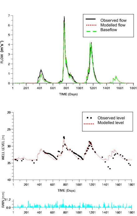
The extended PDM model was first applied to the Lavant catchment using a daily time-step over the period 8 December 1991 to 1 January 1997. Potential evaporation was represented by a simple sine curve over the year with a mean value of 1.4 mm day-1. The calibration to observed flow data gave an R2 value of 0.942 (Table 3), accounting for 94% of the variability in the observed flow series. The simulated flow hydrograph shown in the upper part of Fig. 5 demonstrates the model’s ability to reproduce the ephemeral behaviour of the river, including the inception and cessation time of runoff, as well as the flood peaks. Calibration to the well level data for West Dean Nursery gave an R2 value of 0.854. The well level hydrograph shown in the middle part of Fig. 5 shows very good agreement until the winter of 1995/96. At this point the modelled well levels rise and the River Lavant begins to flow whilst in reality the well levels fall steeply before recovering to normal levels and there is no river flow. This failing of the model is under investigation. The lower graph shows catchment average rainfall in mm over the five-year period.
Note that a formal split sample test involving independent calibration and evaluation periods has not been invoked since there are only three flood peaks over the five-year record. Model performance is regarded as satisfactory on the basis of visual inspection of the hydrographs, paying especial attention to the time of initiation and cessation of runoff, the flood peak magnitude and the shape of the rise and recession of the hydrograph. The R2 statistic has been chosen for presentation here as an overall measure of “goodness-of-fit”; however, other performance measures were assessed, including root mean square error and bias statistics. Comments on the model parameters available for calibration relevant to the robustness of the fitted model are made at the end of this section.
Table 3. Assessment of model performance for the Lavant. Time-step and Objective Calibrated Model
period function (yes/no) performance, R2
Daily Flow yes 0.942
8/12/1991 – 1/1/1997 Well level yes 0.854
15 minute Flow no 0.958
1/8/1993 – 1/9/1994 Well level no 0.985
Fig. 5. Observed and simulated hydrographs of flow and well level depth (m) together with catchment
rainfall (mm) for the Lavant. Daily time-step model for the period 8 December 1991 to 1 January 1997.
Observed level Modelled level Observed flow Modelled flow Baseflow (m 3 s -1 )
The continuous time formulation of the model allows it to be run, without change, at different time-steps. Applying the model at a 15-minute time-step over a 13 month period from 1 August 1993 to 1 September 1994, encompassing the “Chichester Flood” of January 1994, again gave an excellent R2 value of 0.958 in terms of flow (Table 3). This was achieved with the model calibrated using daily data without further adjustment. Assessing the model performance in terms of simulating well levels gave an R2 of 0.985, again using the model parameters obtained from
the daily calibration. The simulated flow and well hydrographs are shown in Fig. 6 along with corresponding 15-minute rainfall totals.
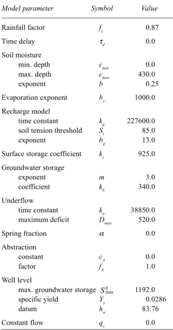
Table 4 shows the parameters of the calibrated model. Worthy of note are the large values for soil tension threshold,
St, and the evaporation exponent, be, which serve to sustain evaporation losses. The adoption of a cubic form for the groundwater storage was based on past experience with the PDM; however, quadratic and linear forms — theoretically more appropriate for non-artesian and artesian conditions
Fig. 6. Observed and simulated hydrographs of flow and well level depth (m) together with catchment rainfall
(mm) for the Lavant. 15 minute time-step model for the period 1 August 1993 to 1 September 1994.
Observed level Modelled level Observed flow Modelled flow Baseflow (m 3 s -1 )
respectively — were trialled but failed to improve performance. The complete knowledge of pumped abstractions from the Lavant and Brick Kiln wells has meant that the abstraction model parameters are set to their nullified values. The external spring component is not invoked as this failed to improve model performance; it might be thought to be accommodated implicitly within the underflow component. This lack of identifiability in conceptual models which incorporate processes known to be operating in a catchment, but for which measurements are not available to support model calibration, is well understood. Whilst the overall model encompasses as many as 21 parameters, many
are included to invoke special forms of behaviour, only some of which will be required for a given catchment. Some parameters can be set to standard values whilst others can be set to nullify the model function they relate to. This results in a model with only a modest number of active parameters for calibration whilst having the advantage of greater flexibility when this is required. Application of the model to ungauged catchments would aim to establish a minimum parameterisation, where possible through establishing physically-based linkages with digital datasets on terrain, soil, land use and geology as exemplified by the approach of Bell and Moore (1998a,b).
Conclusion
The representation of ephemeral flow in conceptual rainfall-runoff models has been shown to require special treatment. Groundwater storages conceptualised as nonlinear storage models, and represented through solutions of the Horton-Izzard equation, require adaptation and extension. Adaptation is required to cater for negative inflows arising when pumped abstractions exceed natural recharge. Extension is needed to represent cessation of flow below a given storage, the build-up of storage deficits, and the subsequent replenishment leading to renewal of flow in the stream channel. Further extensions may be required to accommodate transfers of flow across the topographic boundary of the catchment that are not gauged at the catchment outlet. These include external spring flows outside the catchment’s watershed and underflows beneath the gauging station.
It has been shown how this extended conceptual groundwater storage element can be incorporated in existing rainfall-runoff models, using the PDM model for purposes of illustration. Application to a Chalk catchment in Southern England has served to demonstrate the success of the model in simulating both the intermittency of flow and the flood peak response. Incorporation of well level data into the model calibration process has also shown that good agreement with observed water levels can be obtained. Lack of identifiability of the external spring component served to confirm the well understood difficulty of representing too many processes explicitly in a conceptual model without sufficient observations to support calibration.
The model’s capability of simulation across the full range of flows in permeable catchments means that its utility extends from water resource applications, through real-time flood forecasting, to continuous simulation for land use/ climate change impact assessment and design studies.
Table 4. Extended PDM model parameters for the Lavant
catchment
Model parameter Symbol Value
Rainfall factor fc 0.87
Time delay τd 0.0
Soil moisture
min. depth cmin 0.0
max. depth cmax 430.0
exponent b 0.25
Evaporation exponent be 1000.0
Recharge model
time constant kg 227600.0
soil tension threshold St 85.0
exponent bg 13.0
Surface storage coefficient ks 925.0
Groundwater storage
exponent m 3.0
coefficient kb 340.0
Underflow
time constant ku 38850.0
maximum deficit Dmax 520.0
Spring fraction α 0.0
Abstraction
constant cA 0.0
factor fA 1.0
Well level
max. groundwater storage Sg
max 1192.0
specific yield Ys 0.0286
datum hw 83.76
Acknowledgements
The research has been carried out with the support of the Science Budget of the Centre for Ecology and Hydrology (CEH). Dick Bradford of CEH Wallingford is thanked for discussion of the hydrogeological processes operating in the Lavant catchment. The Environment Agency is thanked for providing the data supporting this investigation.
References
Bell, V.A. and Moore, R.J., 1998a. A grid-based distributed flood forecasting model for use with weather radar data: Part 1. Formulation. Hydrol. Earth Syst. Sci., 2, 265-281.
Bell, V.A. and Moore, R.J., 1998b. A grid-based distributed flood forecasting model for use with weather radar data: Part 2. Case Studies. Hydrol. Earth Syst. Sci., 2, 283-298.
Brunsdon, G.P. and Sargent, R.J., 1982. The Haddington flood warning system, in Advances in Hydrometry (Proc. Exeter Symp.), IAHS Publ. no. 134, 257-272.
Central Water Planning Unit, 1977. Dee Weather Radar and
Real-time Hydrological Forecasting Project. Report by the Steering
Committee, 172 pp.
Centre for Ecology and Hydrology, 2000. PDM Rainfall-Runoff
Model, Version 2.0, CEH Wallingford, UK..
Ding, J.Y., 1967. Flow routing by direct integration method, Proc.
Int. Hydrology Symp., Fort Collins, 1, 113-120.
Dooge, J.C.I., 1973. Linear theory of hydrologic systems, Tech. Bull. 1468, Agric. Res. Service, US Dept. Agric., Washington, 327 pp.
Freeze, R.A. and Cherry, J.A., 1979. Groundwater. Prentice Hall, 604pp.
Gill, M.A., 1976. Exact solution of gradually varied flow, J.
Hydraul. Div., ASCE, 102, HY9, 1353-1364.
Gill, M.A., 1977. Algebraic solution of the Horton-Izzard turbulent overland flow model of the rising hydrograph, Nord. Hydrol.,
8, 249-256.
Greenfield, B.J., 1984. The Thames Water Catchment Model. Internal Report, Technology and Development Division, Thames Water, UK.
Horton, R.E., 1938. The interpretation and application of runoff plot experiments with reference to soil erosion problems. Soil
Sci. Soc. Amer., Proc., 3, 340349.
Horton, R.E., 1945. Erosional development of streams and their drainage basins: hydrophysical approach to quantitative morphology, Bull. Geol. Soc. Amer., 56, 275-370.
Institute of Hydrology, 1992. PDM: A generalized rainfall-runoff
model for real-time use, Developers’ Training Course, National
Rivers Authority River Flow Forecasting System, Version 1.0, March 1992, Wallingford, UK. 26pp.
Institute of Hydrology, 1996. A guide to the PDM. Version 1.0, January 1996, Wallingford, UK. 45pp.
Jones, H.K. and Robins, N.S. (Eds.), 1999. National Groundwater
Survey. The Chalk aquifer of the South Downs. British
Geological Survey Hydrogeological Report Series. British Geological Survey, Keyworth, UK, 111pp.
Lambert, A.O., 1972. Catchment models based on ISO-functions.
J. Instn. Water Engineers, 26, 413-422.
Mandeville, A.N., 1975. Non-linear conceptual catchment
modelling of isolated storm event, PhD thesis, University of
Lancaster.
Moore, R.J., 1983. Flood forecasting techniques. WMO/UNDP Regional Training Seminar on Flood Forecasting, Bangkok, Thailand, 37pp.
Moore, R.J., 1985. The probability-distributed principle and runoff production at point and basin scales. Hydrol. Sci. J., 30, 273-297.
Moore, R.J., 1986. Advances in real-time flood forecasting practice. Symposium on Flood Warning Systems, Winter meeting of the River Engineering Section, Inst. Water Engineers and Scientists, 23 pp.
Moore, R.J., 1999. Real-time flood forecasting systems: Perspectives and prospects. In: Floods and landslides:
Integrated Risk Assessment, R. Casale and C. Margottini (Eds.),
147-189, Springer.
Natural Environment Research Council, 1975. Flood Studies
Report, Vol. 1, Chap 7, 513-531.
O’Connor, K.M., 1982. Derivation of discretely coincident forms of continuous linear time-invariant models using the transfer function approach, J. Hydrol., 59, 1-48.
Posford Duvivier, 1994. River Lavant Flood Investigation. Report Commissioned by National Rivers Authority Southern Region. Smith, J.M., 1977. Mathematical Modelling and Digital
Simulation for Engineers and Scientists, Wiley, Chichester, UK.
332 pp.
Thomson, J.M., Ellis, J. and Headworth, H.G., 1988. South Downs
Investigation. Report on the Resources of the Chichester Chalk Block. Southern Water Sussex Division, 79pp plus figs.
Todd, D.K., 1959. Groundwater hydrology. Wiley, Chichester, UK. 336pp.
Todini, E., 1996. The ARNO rainfall-runoff model. J. Hydrol.,
175, 339-382.
Werner, P.H. and Sundquist, K.J., 1951. On the groundwater recession curve for large watersheds, Proc. AIHS General Assembly, Brussels, Vol. II, IAHS Pub. No. 33, 202-212. Zhao, R.J., Zhuang, Y., Fang, L.R., Lin, X.R. and Zhang, Q.S.,
1980. The Xinanjiang model. In: Hydrological Forecasting (Proc. Oxford Symp., April 1980), IAHS Publ. no. 129, 351-356.
Appendix A:
Solutions to the Horton-Izzard
equation
The Horton-Izzard equation (Dooge, 1973) for a flow per unit area, q
≡
q(t), and an input per unit area u≡
u(t), is(
u q)
q , q> , <b<, = a dt dq b 1 0−∞ − (A.1)where a=mk1/m and b=(m-1)/m are two parameters related
to those of the nonlinear storage equation q = k Sm, where
S
≡
S(t) denotes storage per unit area at time t. This ordinarydifferential equation can be solved exactly for any rational value of m (Gill, 1976, 1977). Recursive solutions are presented here for linear (m=1), quadratic (m=2), exponential (b=1) and cubic (m=3) cases for a constant input
u over the interval (t, t+T), and for the general case when u=0.
LINEAR STORAGE
For m=1 (b=0) the Horton-Izzard equation reduces to the linear reservoir model with the solution
(
e)
u. q e = q -Tk t -Tk T + t + 1− (A.2)This is used in the Thames Catchment Model (Greenfield, 1984) to represent unsaturated soil storage. Werner and Sundquist (1951) and Ding (1967) showed theoretically that the linear form is applicable to flows from confined or artesian aquifers.
QUADRATIC STORAGE
The solution for m=2 for a positive input, u, is
(
)
(
(
)
)
, u q u q + aTu z z z u q t t / t T t − = + − = + 2 / 1 2 / 1 2 1 2 1 1 exp where 1 1 (A.3) or alternatively(
)
{
( )
}
(
q u)
{
( )
uk T}
. + T uk + u q u = q t t 2 T + t 2 / 1 2 / 1 2 / 1 2 / 1 tanh 1 tanh (A.4)This predictive equation forms the basis of the Isolated Event Model (NERC, 1975) and is used in the Thames Catchment Model to represent release from groundwater storage (Greenfield, 1984). Werner and Sundquist (1951) and Ding (1967) showed theoretically that the quadratic form is applicable to flows from unconfined or non-artesian aquifers.
For a negative input, u, relevant when abstractions exceed recharge in groundwater systems, then a valid solution of the Horton-Izzard equation is
( )
(
) (
)
{
tan}
. tan2 -1 q u ukT u qt+T =− √ t − −√ − (A.5) EXPONENTIAL STORAGEWhen b=l (m→∞) in the nonlinear storage model (A.1) then Moore (l983) shows that the model derives from the storage equation
(
+aS)
= q aS + = q γ or expγ log (A.6)where a is the same parameter as appears in (A.1), and γ is an intercept parameter. The solution of the Horton-Izzard equation in this case is
(
) (
) (
)
(
aTu) (
+ q u)
(
(
aTu)
)
. q = aTu u q + u q q = q t t t t t T + t − − − − − exp 1 exp exp 1 (A.7)This is the “log-storage” model, or more properly the exponential storage model, derived by Lambert (l972), and which has been used for flood forecasting on the River Dee (Central Water Planning Unit, l977).
CUBIC STORAGE
When m = 3, so the relation q = k S3 holds, no simple
recursive solution can be obtained. An approximate recursive solution can be developed based on the piecewise linear difference equation solution suggested by Smith (1977, p213). The recursive solution in terms of storage is
(
)
(
2)(
3)
2 exp 3 1 3 1 t t t t T t S kS kS T u kS S+ = − − − − (A.8)from which flow can be predicted as . 3 T t T t kS q+ = + (A.9)
Horton (1945) showed theoretically that the cubic form is applicable to laminar overland flow.
GENERAL STORAGE IN RECESSION
For the recession case when the input, u=0, then the Horton-Izzard equation can be solved for all permissible values of
m and k to give
(
q +abT)
b ; = q -b -/b t T + t 0 1 ≠ (A.10)also for the linear reservoirs case (m=1, b=0), then
(
)
.exp kT q =
qt+T − t (A.11)
Appendix B:
Groundwater abstraction, negative
storage and ephemeral flows
When the input, u, to the nonlinear storage is allowed to be negative and the storage is allowed to develop negative values, with no outflow, then additional theory is required.
Such a case might arise when the nonlinear storage is used to represent a groundwater catchment with input, u, given by natural recharge less pumped abstractions with the possibility of ephemeral flows. Two additional expressions are needed to cater for the transition from the normal nonlinear storage with positive outflow to the case of zero outflow and a simple water balance calculation of negative storage values. If (t, t+T) is the time interval containing the transition then two quantities are required: the time to flow cessation T´ (at time t+T´) and the initial negative storage,
S(t+T). Expressions for these are given below for each type
of nonlinear storage. LINEAR STORE: − − = ′ t q u u k T 1ln (B.1) . ln 1 − + = + t T t q u u k T u S (B.2) QUADRATIC STORE: 2 / 1 1 2 / 1 tan 1 − − − = ′ − u q ku T t (B.3)
( )
2 tan . 1 2 / 1 1 2 / 1 − − − = − + u q u aT uT S t T t (B.4) EXPONENTIAL STORE:This storage is inappropriate for ephemeral flows since positivity of flow is required.
CUBIC STORE: