HAL Id: hal-00318180
https://hal.archives-ouvertes.fr/hal-00318180
Submitted on 20 Oct 2006
HAL is a multi-disciplinary open access
archive for the deposit and dissemination of
sci-entific research documents, whether they are
pub-lished or not. The documents may come from
teaching and research institutions in France or
abroad, or from public or private research centers.
L’archive ouverte pluridisciplinaire HAL, est
destinée au dépôt et à la diffusion de documents
scientifiques de niveau recherche, publiés ou non,
émanant des établissements d’enseignement et de
recherche français ou étrangers, des laboratoires
publics ou privés.
comparisions between CMAM (with interactive
chemistry) and MFR-MetO observations and data
A. H. Manson, C. Meek, T. Chshyolkova, C. Mclandress, S. K. Avery, D. C.
Fritts, C. M. Hall, W. K. Hocking, K. Igarashi, J. W. Macdougall, et al.
To cite this version:
A. H. Manson, C. Meek, T. Chshyolkova, C. Mclandress, S. K. Avery, et al.. Winter warmings, tides
and planetary waves: comparisions between CMAM (with interactive chemistry) and MFR-MetO
observations and data. Annales Geophysicae, European Geosciences Union, 2006, 24 (10),
pp.2493-2518. �hal-00318180�
www.ann-geophys.net/24/2493/2006/ © European Geosciences Union 2006
Annales
Geophysicae
Winter warmings, tides and planetary waves: comparisions between
CMAM (with interactive chemistry) and MFR-MetO observations
and data
A. H. Manson1, C. Meek1, T. Chshyolkova1, C. McLandress2, S. K. Avery3, D. C. Fritts4, C. M. Hall5, W. K. Hocking6, K. Igarashi7, J. W. MacDougall6, Y. Murayama7, D. C. Riggin4, D. Thorsen8, and R. A. Vincent9
1ISAS, University of Saskatchewan, Canada
2Department of Physics, University of Toronto, Canada 3University of Colorado, Boulder, CO, USA
4Colorado Research Associates, Boulder, CO, USA
5Auroral Observatory, University of Tromsø, Tromsø, Norway
6Department of Physics and Astronomy, University of Western Ontario, London, Canada 7National Institute of Information and Communications Technology, Tokyo, Japan
8Department of Electrical and Computer Engineering, University of Alaska, Fairbanks, USA 9Department of Physics, University of Adelaide, Australia
Received: 17 January 2006 – Revised: 16 August 2006 – Accepted: 24 August 2006 – Published: 20 October 2006
Abstract. Following earlier comparisons using the
Cana-dian Middle Atmosphere Model (CMAM, without interac-tive chemistry), the dynamical characteristics of the model are assessed with interactive chemistry activated. Time-sequences of temperatures and winds at Tromsø (70◦N) show that the model has more frequent and earlier strato-spheric winter warmings than typically observed. Wavelets at mesospheric heights (76, 85 km) and from equator to po-lar regions show that CMAM tides are generally po-larger, but planetary waves (PW) smaller, than medium frequency (MF) radar-derived values.
Tides modelled for eight geographic locations during the four seasons are not strikingly different from the earlier CMAM experiment; although monthly data now allow these detailed seasonal variations (local combinations of migrat-ing and non-migratmigrat-ing components) within the mesosphere (circa 50–80 km) to be demonstrated for the first time. The dominant semi-diurnal tide of middle latitudes is, as in the earlier papers, quite well realized in CMAM. Regarding the diurnal tide, it is shown here and in an earlier study by one of the authors, that the main characteristics of the diurnal tide at low latitudes (where the S (1,1) mode dominates) are well captured by the model. However, in this experiment there are some other unobserved features for the diurnal tide, which are quite similar to those noted in the earlier CMAM experiment: low latitude amplitudes are larger than observed
Correspondence to: A. H. Manson
(alan.manson@usask.ca)
at 82 km, and middle latitudes feature an unobserved low al-titude (73 km) summer maximum. Phases, especially at low and middle (circa 42◦N) latitudes, do not match observations well.
Mesospheric seasonal tidal variations available from the CUJO (Canada U.S. Japan Opportunity) radar (MFR) net-work (sites 40–45◦N) reveal interesting longitudinal differ-ences between the CMAM and the MFR observations. In addition, model and observations differ in the character of the vertical phase variations at each network-location.
Finally, the seasonal variations of planetary wave (PW) ac-tivity available from CMAM and the MFR show quite good agreement, apart from the amplitude differences (smaller in CMAM above 70 km). A major difference for the 16-d PW is that CMAM shows large amplitudes before the winter sol-stice; and for the 2-d PW, while both CMAM and MFR show summer and winter activity, the observed summer mesopause and winter mesospheric wave activities are stronger and more extended in height.
Models such as CMAM, operated without data-assimilation, are now able to provide increasingly realistic climatologies of middle atmosphere tides and PW activity. Differences do exist however, and so discussion of the various factors affecting tidal and PW characteristics in atmospheres, modelled and observed, is provided. Other diagnostics of model-characteristics and of future desirable model experiments are suggested.
1 Introduction
In our earlier papers (Manson et al., 2002a, b; Papers 1 & 2), which used CMAM model data from an experiment carried out without interactive chemistry, the emphasis was upon gravity wave (GW) effects, and tides (observed and mod-elled) during the months of January, April, July and October. The parameterized GW drag included that due to topogra-phy (McFarlane, 1987), and the effects of non-orographically excited waves were due to two different schemes (Medvedev and Klaassen, 1995; Hines, 1997a, b). The ozone distribu-tion in CMAM at that time was consistent with the COSPAR International Reference Atmosphere (CIRA, Keating et al., 1990) and the latent heat release from deep convection was due to the parameterization of Zhang and McFarlane (1995). Very briefly, the comparisons of GW spectra in Paper 1 showed, for the first time, the differences in spectral inten-sity between the resolved GW in CMAM and the observed GW from the MF radars at mesospheric heights (72–78 km). For periods less than 2h the differences were substantial (sev-eral orders of magnitude), due to both limited time and space sampling (20 min and 400 km grid spacing). It is not pos-sible to infer, in spectral format, the contribution of GW from the non-resolved parameterized GW. The parameteriza-tion due to Medvedev and Klaassen produced more realistic zonal winds (EW), as shown in latitudinal contour plots for the mesosphere (60–87 km). Regarding the tides, as shown in Papers 1 and 2, the CMAM 12-h (semi-diurnal, SD) tide was quite similar to observations: amplitudes and phases were both often similar, with “Medvedev and Klaassen” tides being more regular than the “Hines-parameterized” results. For the 24-h (diurnal, D) tide agreements were less satis-factory: modeled amplitudes at lower latitudes (≤35 N) and near 80 km were larger than observed in equinoxes; summer mid-latitude values were anomalously large for both param-eterizations; and although phases at low latitudes were quite similar for CMAM and MFR data, at middle latitudes sig-nificant differences occurred for both GW parameterizations. Indeed for this tide the specific tidal models of GSWM (1995 and 2000 versions of the “Global Scale Wave Model”) were better regarding phase variations with season (1 month sam-ples), altitude and latitude. The amplitudes, which in the 2000 version were effectively normalized to satellite vations (UARS-HRDI), were also closer to the radar obser-vations near 80 km.
A new series of experiments using the CMAM with in-teractive chemistry (de Grandpr´e et al., 2000, 1997) pro-vided an opportunity to further assess the model’s capabil-ity in producing realistic tidal and PW fields. It is to be expected that the modifications in ozone distributions, now consistent with the dynamics and radiation, will modify the modelled tides in the mesosphere. The differences in model characteristics are described later in Sect. 2. For the experi-ment described here, 21 years of continuous model data were provided, which allowed us to assess the seasonal variations
of the waves within the mesosphere with 10-day resolution. This allowed demonstration of the seasonal tidal evolutions (amplitudes and phases; 55–88 km) at eight specific locations (these are then combinations of migrating and non-migrating components) for the first time, the assessment of inter-annual variability, and also consideration of longitudinal variabil-ity over the locations of the CUJO (Canada U.S. Japan Op-portunity) MFR network. The latter has allowed consider-ation of the effects of migrating and non-migrating compo-nents. The seasonal mesospheric tidal evolutions shown by McLandress (2002a) are for the migrating components only, due to averaging of satellite data (UARS-WINDII: Upper At-mosphere Research Satellite-Wind Imaging Interferometer) over all longitudes. It is important to reiterate that the tides discussed here are for radar observations at particular geo-graphic locations, and the CMAM tides are also for those same latitudes-longitudes. As such, the tides shown here in-clude both migrating and non-migrating components.
In Sect. 2 the characteristics of the radars and the CMAM are provided, along with description of the common anal-ysis methods applied to both data sets. In Sect. 3, time-sequences for a high latitude location (70 N, Tromsø) from CMAM, MFR and MetO data (UK Meteorological Of-fice, data-assimilation products) are compared, to assess the stratospheric winter warmings and their characteristics. Sec-tion 4 provides spectral wavelets (6-h to 30-d) for CMAM and MFR data and follows that with high resolution variance spectra of CMAM and MFR to investigate the spectral nature of the tidal signals. The seasonal variations and climatologies of tides (12-, 24-h) and planetary waves, along with indica-tions of latitudinal, inter-annual and longitudinal variabilities are given in Sects. 5 and 6, respectively. We conclude in Sect. 7.
2 Description of radars, CMAM, MetO, and data anal-ysis
2.1 MF radars
These systems have been described in Paper 1 and 2, so the comments here are relatively brief. The basic analysis ap-plied to the complex radar signals is the full correlation anal-ysis (FCA) for spaced antenna systems. The variant devel-oped by Meek (1980) is used for several stations (Tromsø 70 N, 19 E, Saskatoon 52 N, 107 W, London 43 N, 81 W, Plat-teville 40 N, 105 W), partly due to its usefulness in dealing with correlograms that are noisier; while the classical method due to Professor Basil Briggs (Adelaide) e.g. Isler and Fritts, 1996), is used at the other stations (Yamagawa 31 N, 131 E, Wakkanai 45 N, 142 E, Hawaii 22 N, 159 W and Christmas Island 2 N, 157 W). Comparisons have shown no significant differences between these methods. The radars provide sam-ples of wind every 2 or 3 km (circa 70–100 km) and 2 or 5 min on a continuous basis. Some loss of data occurs if the
ionospheric scatterers are weak or less numerous, and if the criteria for the FCA are not met. In this paper, the years of 2001 and 2002 were selected as the best years for the MFR data, given the comparative newness of several radars (data from 1994 were retained for the equatorial location, due to their superior quality).
Generally, and based upon data from Platteville, Saska-toon and Tromsø (middle to high latitudes), the observed inter-annual variations of the seasonal positions of tidal max-ima, and of vertical phase structure, are modest (especially evident in the seasonal (12-month) height-versus-time con-tour plots (Sect. 2.4)). However at lower latitudes inter-annual variations of amplitude for the diurnal tide are large near the March equinoctial-maxima and discussions will be appropriately included in later sections (5.2 and 5.4) (Vin-cent et al., 1998; Manson et al., 2002b). The only radar new to the CMAM studies is Platteville, and it along with Saska-toon, London, Wakkanai and Yamagawa comprise the new CUJO network.
Since model-radar wind and tide comparisons are made later, some comment upon the accuracy of the radar-winds is appropriate. Examples of system-comparisons includ-ing MFR, Meteor Wind Radars (MWR), Fabry-Perot In-terferometers, UARS-HRDI (Upper Atmosphere Research Satellite-High Resolution Doppler Interferometer), rockets and radars, have been extensive over the last 10 years e.g. Manson et al. (1996), Meek et al. (1996) and Paper 1. In all of these studies the phases of the tides, or directions of the winds, have generally been satisfactorily consistent (e.g. means within standard errors), as assessed by the au-thors. Most recently we have exhaustively compared MFR and MWR winds data from systems at Tromsø (70 N, 19 E) and Esrange (68 N, 21 E) separated by 200 km (Manson et al., 2004a). The MWR/MFR annual mean ratios were 1.1 at 82 km and 1.1 (summer) to 1.3 (winter) at 85 km. (The larger winter values are thought to be due to a seasonal variation in radar scattering statistics.) The latter is the maximum height used comparatively, in this study. However the mean ratio was 1.6 at 97 km (similar to the HRDI/MFR ratio of Meek et al., 1997), and some mention of that will be made when the MFR amplitudes at the maximum height in the plots are discussed.
There is one last comment to be made. Studies made over recent years (e.g. Papers 1 and 2; Manson et al., 2004c) have shown a tendency for the London wind amplitudes to be somewhat smaller than those at nearby latitudes. Assess-ment of the analysis method used at London, has indicated differences in the algorithm used for the correlograms within the FCA; preliminary wind speed comparisons using two in-dependent analysis systems operating on the same raw radar data sequences, one similar to that used at Saskatoon, has re-vealed a small-bias for London values of 1.2. This correction factor has been applied to some figures in the study (Figs. 2, 4, 9, 11 and 12).
2.2 CMAM
The CMAM is a 3-D spectral general circulation model (GCM) extending from the ground to a height of approx-imately 100 km. The prognostic fields are expanded in a series of spherical harmonic functions with triangular trun-cation at total wave number n=32 (T32) corresponding to a horizontal grid spacing of about 600 km at middle latitudes. The model contains 65 levels in the vertical, with a resolu-tion of approximately 2 to 2.5 km above the tropopause. Re-alistic surface topography, planetary boundary-layer effects, parameterizations of shallow and deep convection, and com-prehensive shortwave (solar) and longwave (terrestrial) radi-ation schemes are all included in the model. The reader is referred to Beagley et al. (1997) for further details.
The finite resolution of CMAM and other GCMs makes it impossible to explicitly represent the effects of GWs with spatial scales smaller than the model grid spacing. (Note that resolved GWs, with scales larger than the model grid spacing, are routinely excited in the model by a variety of sources including shear instabilities and flow over topogra-phy). In order to represent the effects of unresolved (sub grid-scale) GWs on the resolved flow within CMAM and other GCMs, GW drag parameterization schemes are em-ployed. The parameterization of drag due to the breaking of waves excited by sub grid-scale topography is described in McFarlane (1987); this scheme is included in the simulation presented here. The effects of GW that are generated from unresolved non-orographic sources such as moist convection and shear instabilities are represented in this study using the parameterization of Hines (1997b); and its implementation in the CMAM is described in McLandress (1998). A sim-ple Rayleigh-drag “sponge” layer is also employed for the non-zonal part of the horizontal wind field above the 0.01 mb level (∼80 km) in order to prevent the reflection of upward propagating waves at the model upper boundary.
For this CMAM experiment, a comprehensive chemistry package interactively coupled with the radiative and dynam-ical modules has been used (de Grandpr´e et al., 2000). The chemistry module contains 44 species including necessary oxygen, hydrogen, nitrogen, chlorine, bromine and methane oxidation cycle species. Photochemical balance equations are solved throughout the middle atmosphere at every dy-namical time step. A full diurnal cycle is simulated, with photolysis rates provided by a “look-up” table. This ap-proach provides a complete and comprehensive representa-tion of transport, emission, and photochemistry of various constituents from the surface to the mesopause region. A de-tailed comparison of model results with observations (CIRA of 1990) indicated (de Grandpr´e et al., 2000) that the ozone distribution and variability are in good agreement with ob-servations throughout most of the model domain; in the up-per stratosphere the model underestimates the ozone. The vertical ozone distribution is generally well represented by the model up to the mesopause region. Comparisons with
measurements showed that the phase and amplitude of the seasonal variation as well as shorter timescale variations are well represented by CMAM at various latitudes and heights. It was found that the incorporation of ozone radiative feed-back results in a cooling of ∼8 K in the summer stratopause region, which corrects a warm bias that results when clima-tological ozone is used. Realistic ozone concentrations are very important for this present study, as its horizontal and altitudinal distributions are crucial for effective forcing of both semi-diurnal and diurnal solar tides (e.g. Hagan, 1996). We note in conclusion that the present CMAM experiment used the Hines’ parameterization rather than the Medvedev-Klaassen used by de Grandpr´e et al. (2000). It is considered by the authors of the last named paper (private communica-tion) that this is not a significant change and that realistic ozone distributions will be represented within the model data shown here.
CMAM output values have been made available for the locations of the MF radars, with continuous time sequences (10 min samples) over 21 years. Data have been archived at 15 geopotential heights between 55 and 88 km, with a nomi-nal vertical resolution of 3 km.
2.3 MetO
We have also used stratospheric fields of daily (at 12:00 UTC, Coordinate Universal Time) temperature and wind components provided by the UK Meteorological Office (MetO) from the British Atmospheric Data Center (BADC) website at http://badc.nerc.ac.uk. These data have global coverage with 2.5◦ latitudinal and 3.75◦ longitudinal steps and are available for 22 pressure levels from 1000 mbar to 0.316 mbar (∼0–55 km). The description of the original data assimilation system is in Swinbank and O’Neill (1994a) and of the new (November 2000) three-dimensional variational (3D-VAR) system in Swinbank and Ortland (2003); basi-cally, data (now including radiances) are continually incorpo-rated in a global circulation model, and updated atmospheric samples of temperatures, winds and pressure are made avail-able with daily temporal resolution. Systematic errors in the model are reported to be small except near the upper bound-ary where they are attributed to shortcomings in the param-eterizations of gravity-wave drag and radiation. The MetO analyses well represent the major features of atmospheric circulation. For example, the global fields include quasi-biennial and semi-annual oscillations at low latitudes (Swin-bank and O’Neill, 1994b), and the quasi 2-day wave and an inertial circulation (Orsolini et al., 1997).
2.4 Analysis
The analyses used in Papers 1, 2 and in Manson et al. (2003) are also used here, and are applied to both the MFR and CMAM data. The CMAM data are ideal in that there are no gaps, while the MFR data will always have gaps, and there
are criteria which are applied to ensure that all analyses are robust.
To provide seasonal (12-month) plots of atmospheric os-cillations from 5 h to 30 days at a chosen height a wavelet analysis is applied to appropriate years of hourly mean winds with additional data at the ends, if available, to cover the full sliding window for all wave periods used (Fig. 2). A Gaus-sian window of length 6 times the period (truncated at 0.05 of peak value) is used to approximate a Morlet wavelet analy-sis (Kumar and Foufoula-Georgiou, 1997), but one in which gaps do not have to be filled. A Fourier transform (not an FFT) is therefore used and applied to existing data points only. Each time-axis pixel (800 are used) represents several hours, since the axis covers 1 year. Breaks in the heavy data-existence line at the bottom of the frame indicates that there were no data for those hours, and are a warning that spectral data near the edges of, and during, these intervals may be in-accurate. The period scale uses 600 pixels and is linear in the logarithm of the period from 5 to 730 h. Each pixel repre-sents one spectral value, and there is no smoothing. Ampli-tudes are corrected after calculations for attenuation by the window, but on the assumption that there were no signifi-cant gaps. In the plot the value in dB is equal to 20 log10
(wave amplitude in m/s), since this provides a better colour-coverage of the wide range of values.
The spectral analysis method used (Fig. 3) on the hori-zontal winds is the classical periodogram method, but for a non-linear set of frequencies. The purpose is to expand the low frequency portion of the plots.
A common analysis has been used to obtain the ampli-tudes and phases of the monthly diurnal and semi-diurnal os-cillations in the wind field. First, sequences of hourly means were formed. Then for each month of chosen-years for the CMAM data an harmonic analysis was applied to the 28– 31 day time-sequences of hourly values (zonal, E–W; merid-ional, N–S), for the 12- and 24-h oscillations. Contour plots of tidal phases and amplitudes, for heights (55–88 km) versus latitude of the CMAM data, are provided in Fig. 4. Such plots for the MFR data were also shown in Manson et al. (2002a), but the limited data for some locations made these diagrams of only modest value. Here we will simply refer the reader to the height versus time plots for the tides which are derived from the MFR data.
To produce the plots of the tides, for heights versus days of the year, harmonic analysis was applied to 2 day sets of data (55–88 km for CMAM; 61–97 km for the MFR) for in-dividual model and observed years (Figs. 5–10). These data were then vector-averaged into 10 day bins, and smoothing was applied to the phases. The contouring procedure em-ploys a bilinear patch method, viz. the interpolated value is ax+by+cxy+d, where a, b, c, and d are solved from the cor-ner values of a cell. Any pixels representing a value greater than the maximum in the legend are set equal to the maxi-mum. In the case of phase contours, two separate bilinear patch calculations are done, one for cosine and one for sine.
The resulting pair of interpolated values at each point in the cell is recombined to get its phase value. If the phases at cor-ners of the cell have a spread greater than 180 degrees, then no interpolation is attempted since the possibility of multiple solutions cannot be ignored, and the cell is left un-filled.
Finally, an independent planetary wave (PW) analysis is done for selected frequencies, starting with a year of hourly mean data which is extended at the ends, if data are available, to accommodate the desired window length. (It is noted here that for individual radars and a limited number of locations, the PW are recognized by dominant periodicities rather than the equally valuable horizontal wave-numbers.) For the 16-day period (bandwidth 13–19 16-days, Luo et al., 2000) a 48-day window length, and for 2-48-day periods (band-width 1.5–3 days) a 24-day window, are each shifted in 5-day steps over the year (Figs. 11–12). For each of these window-lengths the appropriate mean (48-, 24-day) is removed and used to repre-sent the background wind, a full cosine window (Hanning) is applied, and the Fourier transform is done at the appropriate range of PW frequencies. Gaps are not filled.
3 Stratospheric time sequences (CMAM and MetO) for the Tromsø location (70 N) and choice of data inter-vals
The temporal characteristics of the winds and temperatures at a high latitude station such as Tromsø (70 N), during the winter months, are of great significance dynamically. The drag exerted by breaking planetary waves is responsible for the Brewer-Dobson circulation, with its inherent poleward flow. Enhancements in this circulation lead to “stronger down-welling over the pole, therefore warmer polar temper-atures, and a weaker polar vortex” (Shepherd, 2000). The polar vortex is subject to disturbances (the so-called minor warmings) and breakdowns, as revealed most dramatically in Sudden Stratospheric Warmings (SSW) (Chshyolkova et al., 2006; Manson et al., 2002d; Liu and Roble, 2002; Shepherd, 2000). Further, given the effects of the PW and polar vortex structure (during SSW) upon hemispheric (especially middle to high latitudes) ozone distributions (Randel, 1993; Bald-win et al., 2003) and also upon the temperatures and Bald-winds, and the propagation of various modes into the middle atmo-sphere, tidal characteristics (especially for the 12-h tide) may be expected to be affected for several months of any winter which is experiencing breakdowns during the mid-winter or spring. For example, tidal profiles measured during a SSW changed significantly compared to those for undisturbed in-tervals (Manson et al., 1984).
An earlier study of the variability of the Arctic Polar Vor-tex within CMAM (without interactive chemistry) by Chaf-fey and Fyfe (2001), revealed strong dependence upon the presence of GW parameterization (non-orographic). How-ever, even with its inclusions, the NH polar night jet was somewhat weak, leading to SSW that occurred too often and
too early, and resulting in an unrealistically low potential for PSC (Polar Stratospheric Clouds) formation. The latter play a major role in spring-time destruction of ozone.
For this paper we studied the stratospheric time series of many of the years within the 21 year CMAM data-set, as well as assessing in parallel the wavelets for middle atmosphere altitudes, before choosing a winter (31–32) and years (so-called 31, 32) for inclusion here. These years are generally typical of the entire data set, and they are therefore also used for the tidal and PW characteristics at middle and high lati-tudes that are discussed later. For the radars and MetO, years 2001 and 2002 (with the 2001–2002 winter as focus) were chosen due to availability, quality and quantity of data, and because the year was also generally typical in terms of PW and tidal seasonal variations and their related height struc-tures. However, it will be seen to have one unique mid-winter characteristic. These choices of data-interval are further dis-cussed and justified in Sect. 5.4 (Interannual Variability).
In Fig. 1 we show the MetO and CMAM temperatures for four altitudes from near 20 to 50 km. In this year, observed disturbances do not occur until late December-early January, with another warming pulse late in February. Similar be-haviour occurred at several other 70 N longitudes, and these two warmings also existed in the mean zonal values, sug-gesting a major SSW event. In fact Naujokat et al. (2002) consider this winter, along with 1998/99 and 1987/88, as be-ing interestbe-ing due to them each havbe-ing two SSW events. The existence of two SSW in one winter is highly unusual, and if one calls the 1987/88 second event a “final warming”, the other two years are unique in the Free University Berlin record from 1964. So, indeed, this chosen year was rather special, with a warming as early as late December/January; indeed, we note that by serendipity we have chosen a year with one of the earliest major warmings since 1964, and all others available in the MetO data-set occur later in the winter. However, in contrast, the CMAM time-sequence at Tromsø for model years 31/32 has several disturbances, or warmings, which are seen as departures from the smooth trend toward lower values that began in the late summer and ends in the late spring: these occur as early as November. Most other CMAM years are similar. Notice also that the minimum val-ues in the CMAM stratosphere are significantly higher (10– 30 K) than in the data-driven MetO product.
Thus this figure is consistent with the CMAM study of Chaffey and Fyfe (2001), with frequent warming pulses and warmer stratosphere at high latitudes. Since only one loca-tion was available for this experiment, it is not known if these warmings were seen at all longitudes, and so if any of them were true major SSW.
The PW and/or low frequency wind activity is not shown here, but it is large for model year 31–32 (and generally so for the other years) in the CMAM’s winter 70 N stratosphere: this is consistent with enhanced poleward flows, warmer po-lar temperatures and a weaker popo-lar vortex, which provides a greater likelihood of modeled SSW. The new CMAM data,
Fig. 1. Time sequences of stratospheric temperature data from the United Kingdom Meteorological Office (MetO, or sometimes
UKMO) and the CMAM model. The location is Tromsø (70◦N)
and the years are 2001/02 and model-years 31/32.
influenced by internally calculated ozone, has not changed this scenario. A more global assessment, involving more longitudes, of PW activity within CMAM is desirable; the strength of the zonal vortex from 30–100 km requires a com-bination of PW and GW to establish realistic middle to high latitude summer and winter vortices, with the GW closing or reversing the vortex in the mesosphere. If PW effects are too large, then GW fluxes required to establish realistic mesopause temperatures will be different from the “real” or typical atmosphere. There will be implications for the mod-eled tides and planetary waves at MLT altitudes.
4 Spectra of winds: wavelets and periodograms
Here we provide wavelets for the complete set of MFR loca-tions, including the 40 N CUJO network. The contour plots are again for the year 2001/02 (MFR) and model year 31/32 (CMAM), and cover 12 months of the split (winter-centered) year and periods from 6-h to 30 days. (The varying time in-tervals for each spectral estimate are approximately 3 times the period of the respective wave). Figure 2 is for 85 km, and brief comments are made upon spectra at 50 km (using MetO) and 76 km (MFR).
We consider, firstly, the general strengths of the spectral features in Fig. 2. The CMAM 24-h tides are larger than the MFR at Hawaii (at which latitude the diurnal tide dominates the tidal fields, Paper 1), and the CMAM 12-h tides are often (e.g. winter) larger than the MFR at Saskatoon and Tromsø (where the semi-diurnal tide dominates the tidal fields, Pa-per 1). In both cases the differences are typically two color (contour) steps (6 dB, a factor of 2). We remind the reader at this stage that the MFR winds near 85 km are probably small by up to circa 2dB (Sect. 2), which often would involve a change of one color step, but even with that, the tidal am-plitude generalizations above are still true. Considering the PW (i.e. low frequency) portion of the spectra, the CMAM intensities have already decreased from their maxima near 67 km (wavelet not shown), and the MFR values are, at most locations, larger than modeled by up to one color step (3 dB). Again allowing for the small-bias (circa 2 dB) in the MFR winds near 85 km (Sect. 2), the “corrected” observed PW in-tensities would be up to two color steps larger (factor of 2). These differences are made more quantitative in Sects. 5 and 6.
There are evidently also seasonal differences between the CMAM and MFR tidal amplitudes at 85 km e.g. the modeled 12-h tides at Saskatoon have a stronger maximum in winter-centred months (November–March) than is observed, and the modeled monthly 24-h tides at Christmas Island vary quite differently from observed. Regarding PWs, both CMAM and MFR evidence a clear preference for longer periods in winter-centered months. Peaks in the 10–20 day periods can be associated with the Rossby or “normal” modes (the so-called 10- and 16-d PW). Again, these differences between modeled and observed values will become more obvious and quantitative in the tidal and planetary wave contour plots (height versus time) of the next sections.
The higher spectral resolution available for a periodogram analysis proves to be useful in further typifying the tidal features. We have chosen the autumn days (September– November) for the middle latitude location of Saskatoon, where the 12-h tide often dominates (Fig. 3). 12 day intervals are slid by 2 days to show the spectral features as they evolve [this compares with ∼3 day intervals for the tidal features in the wavelets.] The MFR spectra reveal the normal burst of 12-h tidal energy regularly observed at this time (Manson et al., 2003); here the spectral peak is clean with no indication
Fig. 2. Wavelet analysis of 85 km zonal wind data from the MF radars and from the CMAM model: the locations are those of the MF radars, Christmas Island to Tromsø. The years are the same as for Fig. 1: 2001/02 and model-years 31/32. Data amplitudes from London’s MFR are multiplied by a factor of 1.2 due to a bias in the local analysis.
of other peaks or side-lobes near the main feature. How-ever, for CMAM (again using model year 31) after the au-tumn burst (which is rewarding and unusual to see success-fully modeled), the spectral noise from 16 to 10 h is consid-erable. Side-lobes in this spectral region have been shown to be largely due to non-linear local interactions between the tides and 10- and 16-d oscillations associated with Rossby PW activity (Manson et al., 1982). As the spectra show, the PW activity at these times was low. Such spectral behaviour is seen at all locations, and for the 24-h tide at low latitudes. This is interesting and perplexing. It raises the possibility that the GW-tidal interactions are modifying the phases and hence apparent frequencies of the 12-h tide (Walterscheid, 1981).
5 Tides: seasonal variations in the mesosphere
In our earlier Papers 1 and 2 using CMAM data, contour plots (height versus latitude), were assessed for the middle month of each season (January, April, July, October). Lo-cations ranged from Christmas Island to Tromsø, with only Tromsø being outside a restricted longitudinal range from the Pacific to western North America). 12- and 24-h amplitudes and phases were shown. Briefly, the modeled tides had ma-jor features similar to those observed: the 24-h tide domi-nated at low latitudes, with maxima in equinoxes and short wavelengths (25–30 km); there were generally long wave-lengths (∼100 km) at high latitudes. The 12-h tide dominated at higher latitudes (>40◦), with winter amplitudes at 85 km
Fig. 3. Spectral analysis of zonal wind data from the MF radar at Saskatoon and from the CMAM model. See Sect. 2.4 for the analysis method and discussion.
above 10 m/s, and wavelengths of moderate size (50 km); wavelengths were longer (∼100 km) in summer, and 40– 80 km in the equinoctial months of April and October; am-plitudes were smaller (5–10 m/s) in the chosen non-winter months.
However, some significant differences were also found be-tween the model and the observations, involving the 4 cho-sen seasonal months, latitude and altitude. There were also some differences in the modeled tides and mean winds, de-pending upon the use of the Hines or Medvedev-Klaassen GW parameterizations. We summarized these as follows: the modeled 12-h amplitudes and phases were in generally good agreement with the MFR observations, with the Hines parameterization showing more phase irregularities than the Medvedev-Klaassen parameterization; the modeled 24-h
am-plitudes for equinoctial low latitudes and summer middle lat-itudes were significantly larger than observed near 82 and 73 km, respectively, allowing for the probable MFR speed bias; and modeled 24-h phase-gradients (wavelengths) and absolute phases, while similar to observations at low and high latitudes, differed quite significantly at middle latitudes (<52◦N). In the 24-h case, there were significant differences
at certain times and latitudes for tides from the two parame-terization schemes.
5.1 Latitudinal contour plots (latitude verses height) We formed such seasonal contours (middle months) for sev-eral years of the 21 now available, and noted that although the major features were robust, the inter-annual variability
was of similar magnitude to that found earlier between the two parameterizations when applied to a single year. The phase contours for different years were often smoothly vary-ing with latitude, suggestvary-ing that the earlier claim (Paper 1) that the Hines parameterization produced more phase dis-continuities may have been based upon a small data sam-ple. The most useful presentation for this format, where rel-atively modest changes at a given location can lead to sig-nificant changes (visually very evident) in the continuity of latitudinal contour-patterns, was therefore determined to be an average of the 21 years for each of the 6 locations chosen: Christmas Island, Hawaii, Yamagawa, Platteville, Saskatoon, and Tromsø. (3 Pacific, 2 Canada-U.S., 1 Scandinavia). The average amplitudes and phases are from the vector means of the tidal vectors for each year. The zonal wind plots for both tides, with amplitudes and phases, are show in Fig. 4; the phase structures shown are common to many of the in-dividual years of 21, and the meridional plots (not shown) are very similar in structure and values (the amplitudes in the equinoxes are less than 5 m/s smaller). As noted earlier, the MFR data do not provide useful complementary plots due to data gaps (time or height, Paper 1), so the discussion be-low will refer to our earlier CMAM papers, and on occasion to the seasonal contour plots (height versus time, below) for Saskatoon and Hawaii.
The contour plots of Fig. 4 are very similar in general structure, amplitudes and phases to those from the previous CMAM experiments (Paper 1, with non-interactive chem-istry), so that the major features of similarity with observa-tions are again clearly evident, as are the differences. These amplitude differences will be considered in more detail in Sect. 5.2.
As in Papers 1 and 2, and especially in the equinoxes, the modeled vertical phase gradients of the 24-h tide in Fig. 4 change from large (λ∼22 km) at low latitudes to small (λ of order 100 km) at latitudes near Saskatoon (52◦N) and be-yond; this is reasonably consistent with the expected domi-nance of the S (1, 1) and S (1, −1) Hough modes (λ∼28 km and >100 km). Since the general phase-behaviour shown in Fig. 4 is similar to that previously modelled (as in Papers 1 and 2), and therefore CMAM vertical phase-gradients at mid-dle latitudes will again differ from observations, we will dis-cuss this matter in more detail in Sect. 5.2 using tidal contour plots for two locations.
Regarding the tidal characteristics, it will be shown be-low that the seasonal changes (modelled and observed) are quite large, and other maxima appear in tidal contour plots when higher temporal resolution (circa 10 days) is used. One month from a season is not enough to characterize seasonal variations. At this point we remark that the similarity of tidal characteristics between those in Fig. 4 and those in Paper 1 is rather surprising given the interactive-chemistry of this present experiment. Modelled ozone distributions, with more realistic vertical distributions (de Grandpr´e et al., 2000), were expected to provide more realistic forcing of the
tides, in comparison with those from a model with imposed ozone distributions; again, the 12-h tide, for which ozone dominates the forcing, might have been expected to show more changes than the 24-h tide. The changes in ozone have evidently been small at those heights responsible for tidal forcing of the various Hough modes.
5.2 Annual contour plots (height vs. time) at Saskatoon (52◦N) and Hawaii (22◦N)
We now move to comparisons of CMAM and MFR tides for two locations (Hawaii and Saskatoon) which are, respec-tively, dominated by the diurnal and semi-diurnal tides. For the first time we can show 10-d resolution for the modeled height-time contour plots throughout the year. The selection of year 31 from the CMAM set of 21 years was made because it has been featured in the previous figures, and because in the contour plots of this section the inter-annual variability leads to quite small changes in seasonal and altitudinal pat-terns of amplitude and phase changes, at these two locations i.e. changes that are small compared to those that will be demonstrated between CMAM and the observations. In this, year 31 is quite typical tidally, as is the observed year of 2001 for the MFR data. However, there may still be significant inter-annual variability of amplitude within the regions of lo-cal amplitude maxima, and these will be discussed below at appropriate points, as well as in Sect. 5.4.
In Figs. 5 and 6 we show a comparison of CMAM and MFR tidal amplitude and phase data respectively, for 365 days, using harmonic 10-d fits. The analysis was described in Sect. 2. Color/contour scales are chosen for best comparisons of the extreme differences between 52 and 22◦N. Please note
that the radar data are extended to 97 km to demonstrate the evolution into the lower thermosphere, while CMAM is limited to 88 km, and is best considered to 82 km, to avoid boundary effects.
For the 24-h (diurnal) tide at Hawaii (Fig. 5), modeled equinoctial values at 82 km reach maxima of 38/53 m/s in April/September for the NS component, and 48/44 m/s in April/September for the EW component. Meanwhile ob-served values in February–March/September are 19/22 m/s for the NS, and 15/19 m/s for the EW. We also calculated the mean values of the equinoctial features for five years of CMAM and MFR tides and found little difference be-tween those and the plotted values for years 31 (CMAM) and 2001. It is worthy of note that the spring maxima occur about one month later in CMAM plots than in the observed MFR plots. However, using the values above, the ratios of the CMAM/MFR amplitudes range from 2 to 3. Allowing for a speed bias (small) of 1.3 for the Hawaiian MFR (based on recent comparative data (2005) from Steven Franke) the corrected ratios become 1.5 to 2.3. We note that the equinoc-tial maxima values from GSWM-2000 (Paper 2), which were normalized to UARS-HRDI values at 95 km are also smaller (they are circa 25 m/s) than CMAM at 82 km.
Fig. 4. Latitudinal contour plots (latitude verses height) of CMAM tidal amplitudes and phases (zonal component), which result from harmonic analysis (Sect. 2.4). The locations are Christmas Island, Hawaii, Yamagawa, Platteville, Saskatoon and Tromsø. 21 years of data are used, with model-years 28–48.
A final remark about Hawaiian tides in Fig. 5: the equinoc-tial MFR values maximize (circa 35 m/s) near 90 km but are only near 24 m/s at 96 km. Certainly the GSWM and
CMAM values shown in Paper 2, and in Fig. 5, continue to increase above 82 km. From Manson et al. (2002c), satellite-derived diurnal tidal amplitudes over Hawaii in the autumn
Fig. 5. Annual contour plots (height versus time) of diurnal and semi-diurnal tidal amplitudes resulting from harmonic analysis of CMAM
(year 31) and MF (year 2001) radar data for Saskatoon (52◦N) and Hawaii (22◦N), and providing 10-day resolution. Interpolation between
Fig. 6. Annual contour plots (height versus time) plots of diurnal and semi-diurnal tidal phases resulting from harmonic analysis of CMAM
(year 31) and MF (year 2001) radar data for Saskatoon (52◦N) and Hawaii (22◦N), and providing 10-day resolution. Interpolation between
are typically 35 m/s at 96 km, which provide a HRDI/MFR speed ratio of nearly 1.5. (HRDI: High Resolution Doppler Imager on UARS.) This is the expected speed bias ratio pre-sented in Sect. 2.1, so that the MFR amplitude-decreases above 90 km in Fig. 5 are artificial (intrinsic to the MFR sys-tem).
The remaining diurnal tidal feature occurs in the mid-latitudes in summer. At Saskatoon, the modeled 73 km max-ima (circa 24 m/s) are not observed and typical values there are only ∼6 m/s. There are no MFR speed biases, compared with Meteor (MWR) radar, at 73 km, so these interesting dif-ferences in Fig. 5 remain.
For the 12-h tide, both CMAM and MFR data demonstrate maxima at the higher latitude location and generally have similar seasonal variations at 52◦N: modeled/observed win-ter values near 82 km are 14–18/8–10 m/s (beyond the speed-bias expectation), and the late-summer to autumn maxima are well modeled (16–20/14–18 m/s). Other models have not shown this dominant feature well (cf. Paper 1, 2; Riggin et al., 2003).
In Fig. 6 we compare the phases for tides, between the lat-itudes of 52 and 22◦, and between the CMAM and the MFR observations. The phases are more revealing than the ampli-tudes, as they suggest the tidal Hough modes that are dom-inant. For the 24-h tide, CMAM provides very strong ver-tical phase gradients (λz∼22 km) at Hawaii, and weak
gra-dients (λz>100 km, evanescent) at Saskatoon: as noted
ear-lier, reasonably consistent with S (1,1) and S (1,−1) Hough modes (λz∼28 km, and evanescent, respectively). The tidal
winds are clockwise rotating, and in quadrature as required for dominant modes. Observationally the contrast in vertical wavelengths is less pure: for Hawaii vertical wavelengths (at 75–90 km altitude) are closer to 30–32 km during the sum-mer, and somewhat longer in the winter, again with the com-ponents in quadrature; and for Saskatoon they are relatively short in winter (∼50 km near 85 km altitude) and irregular in summer (the NS, EW components are out of phase below 80 km, and in phase near 90 km.) These observed features are very consistent with earlier studies (Paper 2), and are not unique characteristics of the chosen year (2001). The ob-served phase structures are indicative of a mixture of tidal modes, which is also seasonally varying. This is consis-tent with the longitudinally varying tidal structures and non-migrating tides shown from the HRDI winds (Manson et al., 2002c, 2004b). Unfortunately, the available CMAM data does not allow for zonal wave-number analysis. Finally the colours for the phase-plots are often similar when compared between CMAM and MFR, which is consistent with the sim-ilarities in the phase profiles discussed above (as concluded in Papers 1 and 2).
The above may seem to be overly critical of the ability of CMAM to simulate the diurnal tide, and that impression should be corrected to some degree. It is appropriate to com-ment on the two papers on the 24-h migrating tide by McLan-dress (2002a, b). They discusses the simulation of the tide
in the extended CMAM, mainly at low latitudes (<40◦), and
notes that the following are reproduced: the semi-annual am-plitude variation (near 20◦); larger tides in March/April than
September/October (especially for the EW component) and generally very good agreement with amplitudes observed by WINDII at 96 km; a 4- to 6-h shift in phase from winter to summer (NH); and other SH-NH differences we need not comment upon. Indeed the CMAM data shown in Figs. 5 and 6 also show these features, which are often not revealed by other models. Other models e.g. GSWM-2000, depend upon GW drag or variations in eddy diffusion to produce this 6 month variation; while the author goes on to demonstrate that the effects of parameterized GW and planetary waves are less important than the effects of both heating (maximizing at the equator in the equinoxes) and mean winds (latitudinal shears in the summer mesospheric easterlies).
The difference between observations and model that we have demonstrated here are at a further level of subtlety: monthly vertical phase gradients at a particular location (Hawaii) where non migrating tides become an issue (Man-son et al., 2004b) in modifying the pure S(1,1) mode, (that mode is dominant in satellite data when longitudinally aver-aged); and assessments of vertical phase gradients at higher latitudes (≥40 N), where the decay of the S(1,1) mode with latitude and the growth in influence of evanescent modes be-comes important. These features are robust and are not a fea-ture of the chosen year (2001). We discuss the decay of the S (1,1) mode in the next section where longitudinal effects near 40◦are considered.
Now, considering the 12-h tide in Fig. 6, the observed and modeled tidal phases are rather similar, as the color ranges for each component and location are evidently similar, especially at 52 N. CMAM provides medium wavelengths (λz∼50 km) for Saskatoon, albeit with somewhat irregular
gradients in height and time, during the winter, and longer or evanescent structures in summer above ∼60 km altitude; the phase gradients are rather irregular in height and time at Hawaii, with wavelengths ranging from short (λ∼50 km) to long (>100 km). The Saskatoon winter tidal components are in quadrature. Observationally, the phase structures at Saska-toon are very regular, again with medium wavelengths (∼40– 45 km at 70–97 km) in winter, but now with short/long wave-lengths (∼30/>100 km) below/above 80 km altitude in sum-mer; while for Hawaii the wavelengths are variable in time and height (and between components), as modeled. (The NS Hawaiian contour plot is very similar to the model, while the winter-EW differs strongly in the low altitude regions of large MFR amplitudes (Fig. 5)). Overall, and as in the first CMAM experiment (Papers 1, 2) the 12-h tide is better sim-ulated than the 24-h.
5.3 Longitudinal variability over CUJO
Although the high temporal resolution CMAM data were not available over a full range of longitudes at any latitude,
Fig. 7. Annual contour plots (height versus time) of diurnal (24-h) tidal phases for the three CUJO network locations near 45◦N, from both the MF radar observational systems and from CMAM. Zonal (EW) and meridional (NS) components are shown.
data for the CUJO network were provided. We have already demonstrated, using MFR data, that the longitudinal vari-ability (London, Platteville and Wakkanai) of the wavelets (tidal to planetary waves) is significant (2000–2001) and that non migrating tides (NMT) are quite evident (Manson et al., 2004c). We have also shown, in this study, wavelets for 2001–2002 for these locations, and the differences between Eastern Canada and Japan were again evident (Fig. 2). Here
we show the annual tidal contours (height versus time) for these three locations from both the MFR observational sys-tems and from CMAM, and for 24 and 12-h (Figs. 7, 8).
Considering the 24-h tide (Fig. 7), the observed phase gradients are strikingly different across CUJO, especially in summer for NS component. However, the CMAM varia-tions are also considerable at particular heights and times. The global HRDI analysis evidenced strong NMT activity
Fig. 8. Annual contour plots (height versus time) of semi-diurnal (12-h) tidal phases for the three CUJO network locations near 45◦N, from both the MF radar observational systems and from CMAM. Zonal (EW) and meridional (NS) components are shown.
(Manson et al., 2004b) especially at wave-number -3 (east-ward propagation), which was associated with the observed longitudinal structure (amplitude and phase) of the tide (wave-number 4). There are also substantial differences be-tween model and observations at each site, (the plots are ver-tically offset so comparisons are easily made) from which the observed strong vertical gradients indicate a larger influence of S (1,1) mode than modelled. The observed influence of
the S (1,1) was much less at Saskatoon (52◦N versus 40◦N, Fig. 6). Modelling and theoretical studies show that the dis-sipation associated with eddy diffusion increases the vertical wavelength of the S (1,1) mode in the mesopause region, and broadens the tidal structure to higher latitudes: coupling into the S(1,−2) and (1,−1) modes occurs as the S(1,1) mode is damped (Vial and Forbes, 1989).
Fig. 9. The vector-differences between the measurements and the fit of a wave equation for the three CUJO MF radars, and for CMAM at those locations, have been calculated and expressed as power: this unfitted power represents the non-migrating tides (plus noise). The wave equation is applied for both the diurnal and semi-diurnal migrating tides (m=1, 2). As in Fig. 2, data amplitudes from London’s MFR are multiplied by a factor of 1.2 due to a bias in the local analysis. Red represents almost total dominance of the migrating tide. Zonal (EW) and meridional (NS) components are shown.
Finally, for the 12-h tides (Fig. 8), there are evidently generally strong similarities between the three CMAM con-tours; for both components, the plots are offset vertically so comparisons are more easily made. The observations show somewhat greater longitudinal differences in phase e.g. compare the colours of early and late winter months above 90 km (EW and NS components) for Wakkanai and Lon-don, and also the colour-differences in the summer months for both components. These observed phase differences across CUJO are consistent with our analysis of HRDI winds, which evidenced significant longitudinal semi-diurnal tidal structures and the related NMT components (Manson et al., 2004b); these are thought to be due to orographic-related solar-forcing and stationary planetary waves (n=1). Ward et al. (2005) have published results from the extended CMAM version. The NMT compare well in terms of amplitude with
existing observations e.g. HRDI-UARS, although a phase er-ror renders the wave-number 2 features in their Fig. 2 incor-rect (W. Ward, private communication) and a corincor-rection is in process. Finally, notice that the differences between model and observations at each site in CUJO are quite noticeable, consistent with some differences in tidal mode-composition. E.g. the presence of a higher order mode, which is consis-tent with the large observed phase gradients, at low heights in summer.
The above has been based upon visual comparisons, and color-pattern recognition: the differences show up very well. However, an alternative quantitative measure of longitudinal change is now described. The wave equation for the diur-nal and semi-diurdiur-nal migrating tides (m=1, 2) is fitted to the data from the three CUJO sites (CMAM or MFR). The vec-tor differences between the measurements and the fit are then
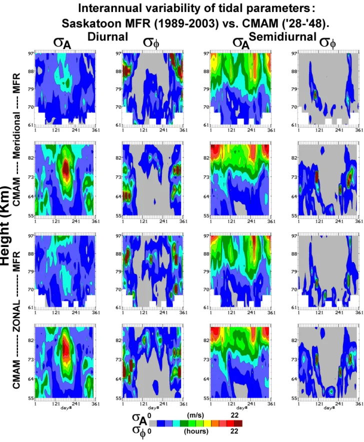
Fig. 10. Interannual variability of tidal parameters as represented by the standard deviations of the tidal (24-, 12-h) amplitudes and phases
for both components (zonal, meridional) and for CMAM and the MFR at Saskatoon 52◦N: 21 years of CMAM are used, and 15 years of
calculated, and expressed as power: this unfitted power rep-resents the noise and non-migrating tides. In Fig. 9, red (90– 100%) represents almost total dominance of the migrating tide, while greens and blue indicate non migrating tides (and noise). The offset and linking lines again indicate the height interval in common between CMAM and MFR. Given the differences in phase structures between CMAM and MFR in Figs. 7 and 8, it is expected that the regions of migrating tide dominance would also vary in height and time, and in-deed they do. For the 12-h tide it is not easy to say which (model or observation) has more migrating tide dominance. CMAM does have considerable yellow and red areas below 76 km in summer, indicating migrating tide dominance: how-ever the phases there (Fig. 8) show no change with height, while NS observations at Wakkanai and Platteville indicate a very strong gradient and hence a combination of Hough modes (55 km–88 km). These short summer wavelengths be-low 76 km were also observed at 52◦N in Fig. 6. The low
altitude and long wavelength summer migrating tide domi-nance in CMAM (Fig. 9) is therefore unlikely to be a real feature. A similar feature in the CMAM and MFR plots of Fig. 9 is the dominance of the migrating tide (yellow and red) in the region of late summer-fall maximum amplitude above 80 km; this amplitude feature was seen in the annual CMAM and MFR contour plots of Fig. 5, as well as over CUJO.
For the 24-h tide, there is a clear tendency for the migrat-ing tide’s dominance in Fig. 9 to occur in the equinoxes for the MFR data, at which time the S (1,1) mode maximizes at tropical latitudes and extends its influence to CUJO lat-itudes. The evidence for this was just noted from Fig. 7. While the migrating tide’s dominance is also true for CMAM in the meridional NS component, it is not true above 76 km for the fall’s zonal EW component. At this very time, there is no CMAM tidal maximum amplitude evident over CUJO (figure not shown), although one exists for the spring. The dominance of the migrating tide in CMAM extends down to 55 km for late spring and early fall, but we have no data from the MFR to verify details of that.
5.4 Interannual variability
Here we have calculated the standard deviations of the tidal (24-, 12-h) amplitudes and phases for both components and for CMAM and the MFR at Saskatoon (Fig. 10): 21 years of CMAM are used, and 15 years of MFR. Comparisons with the amplitudes of Fig. 5 for a particular year show extra-ordinary similarity between MFR and CMAM amplitudes and their standard deviations (s.d.). All of the regions of large amplitude in the earlier amplitude plots provide regions of large s.d., as expected if there is strong similarity of position for the dominant amplitude seasonal–height structures year-by-year, and variances are proportional to the magnitude. This indicates that the observed contour plots for year 2001 and modelled year 31 are typical of the 15/21 year data sets. As examples, the late summer-fall 12-h amplitude structures
seen above 80 km in both CMAM and MFR annual contour plots (Fig. 5) has a similar height-date location each year, but the amplitude of the feature evidences interannual variability as indicated by the s.d. maxima; and the unobserved summer 24-h amplitude maxima also provides a striking maxima in the s.d. plots.
The phase comparisons are also interesting. For the 12-h tide, the model and observations (Fig. 10) illustrate that s.d. values are largest during the times and heights of rapid phase change in the spring and autumn (Fig. 6). This is to be ex-pected. However the s.d. values are also large in CMAM during winter for regions near 73 km. The phase changes were large there even during the single sample year of 31 (Fig. 6), since contour-continuity was not achievable (blank areas in the figure). This is a significant difference from ob-servations, and may again indicate GW interactions with the tidal field (Sect. 4, Fig. 3). However, overall the similarity in these plots between CMAM and MFR data-sources testi-fies to significant similarities between their respective tidal characteristics at middle-latitudes; and inherently, that inter-annual variability of tidal amplitude and phase structures is modest. This further justifies the choice of individual years for this study (Sect. 3).
The 24-h tidal phase s.d. contour values (Fig. 10) also demonstrate maxima in regions of greatest observed (MFR) phase gradients (Fig. 6) and in doing so indicate that the ob-served contour plots for year 2001 are typical of the 15 year data set. There are clear s.d. maxima near 85–88 km in winter time (this was earlier noted to be due to the influence of the S (1,1) mode), and in mid summer for the zonal (EW) com-ponent where the vertical phase gradients (Fig. 6) are also large.
In contrast the largest s.d. phase values are at lower heights (64–73 km) for CMAM in winter, whereas the phase gra-dients for year 31 (Fig. 6) do not have large values. This indicates large inter-annual variability in CMAM at these heights, as there are also amplitude s.d. maxima near there in Fig. 9. These phase variability plots confirm the differ-ences noted earlier between CMAM and MFR-derived tides at middle latitudes.
5.5 Discussion of the modelled tides in CMAM
The remarks here are brief. The seminal papers on tidal the-ory and modelling (e.g. Forbes, 1982a and b) demonstrate the atmospheric characteristics which lead to seasonal and latitudinal variations in the tidal phase-gradients (related to mixtures of Hough modes) and amplitudes. Meridional (NS) gradients in middle atmosphere temperatures and mean zonal winds, along with eddy diffusion processes, lead to Hough mode coupling and additional contributions by these higher order modes to the resulting tidal climatologies. Planetary and gravity waves (Sect. 3) play dominant roles in establish-ing these wind and temperature fields. Changes in ozone and water vapor distributions (height and latitude) also directly
force different Hough modes in various seasons and during disturbed conditions e.g. SSW. In so far as CMAM, or any generic GCM, have globally varying characteristics of winds, temperatures, ozone or water differing from the real atmo-sphere in the decades of the comparisons, there will be dif-ferences in the modelled and observed tides.
The fact that the differences for CMAM are small, or lim-ited to a few features, indicates that CMAM includes the dominant physical, radiative and dynamical processes. Very focused GCM experiments will be needed to establish the atmospheric characteristic which is the cause of any partic-ular difference between model and observation. Tides are the probably the most demanding of any dynamical feature to successfully model, but there is reason to believe that fur-ther modelling experiments can improve both tidal modelling and our understanding of atmospheric processes in general. There are further remarks in the Sect. 7.
6 Planetary waves, annual height-time contour plots (16-, 2-d)
6.1 16-d planetary wave
It was already shown, in the wavelets of Fig. 2 and discussion in Sect. 4, that the amplitudes for periods greater than 10-d at both 76 and 85 km were greater in the observed (MFR) than in the model (CMAM) data. The height (circa 60–90 km) versus time (months in 2001–2002 and in model years 31– 32) contours of Figs. 11 and 12 show this in more detail. In comparing model to observation we must be careful to consider only the general level of activity and not particular time-height “events”, as the model is free-running and not a data-assimilation system.
In CMAM (Fig. 11, left side) we note large amplitudes (∼13 m/s) as early as November and re-occurring in bursts until March–April. The amplitudes are large from 55–75 km in winter-centered months and then from near 75 km to the top of the summer’s westward jet (∼87 km). There is evident contour-similarity at the three CUJO sites near 40◦(London, Platteville and Wakkanai). We show EW amplitudes, and these dominate over the NS (not shown), as expected for this normal (PW) mode. This pattern of pre-winter solstice ac-tivity was seen in the 8 other model years after year 31 that were assessed (32/33–40/41).
The observations (Fig. 11, right side) are significantly dif-ferent: the winter amplitudes are largest later in the winter (January–March) for the three 40◦CUJO locations; the
win-ter amplitudes remain large up to near 90 km; there is signif-icant longitudinal variability (e.g. Wakkanai and Platteville in March) as already noted by Luo et al. (2000, 2002a, b) and Manson et al. (2004c); and the summer contours (max-ima near 80 km) vary more in timing and heights than for CMAM. Luo et al. (2000) compared 10 years of such 16-d PW activity at Saskatoon, and found that 7 of 10 years had
greater amplitudes later in winter; there was also significant variability in the size and placement of the summer maxima near the zonal wind reversal. Also note the observed maxi-mum height of the summer’s westward jet is lower (∼80 km) and more variable (see Wakkanai at 85 km) than the modeled heights.
Comparing observations with model, we note that the MFR 16-d PW amplitudes are comparable or larger than CMAM at comparable heights, even without allowing for the MFR bias toward smaller values. There may be differ-ences in the damping of these normal (resonant) modes, with height, between the real and modeled atmospheres. Mech-anisms in CMAM include radiative damping and eddy dif-fusion. The real atmosphere may also be offering mod-est barotropic or baroclinic instability at the 75–90 km lev-els (Andrews et al., 1987) which would enhance the ob-served waves. There could also be less geophysical forcing of these modes in the early winter of the real atmosphere. Meyer and Forbes (1997), using the 2-D Global Scale Wave Model (GSWM), showed that longer period PW (>10 d) are strongly damped above 90 km, due to Newtonian cooling, molecular viscosity and ion-drag (the latter being dominant). Another possibility for the larger mesospheric PW am-plitudes (or activity) in CMAM in early winter (Novem-ber, December) could be the strength of the modeled win-ter vortex. From Charney and Drazin (1961) and Manson et al. (2005), weaker eastward flow (u) leads to smaller intrinsic phase velocities (u-c) for the 16-d PW (westward propagat-ing), a decreased chance of this (u-c) exceeding the “limit-ing speed” (this later is inversely proportional to the squared wave-numbers) and a resulting larger amplitude for verti-cally propagating waves. In fact, the CMAM zonal winds at 55 km (Fig. 11, and the 8 other model years) in Novem-ber/December are 20–30 m/s weaker than those in CIRA (1986). These are heights where CIRA is at its most reliable. Thus PW propagation into the mesosphere is favored within CMAM during the early months of the winter-season’s east-ward flow. The mean winds (CIRA) are more similar to CMAM in January/February when the PW amplitudes (or wave activity) from CMAM and the MFRs at 70 km are more similar (Figs. 11 and 12). This factor may well explain the discrepancy between modeled and observed PW activity in the mesosphere early in the winter months.
6.2 2-d planetary wave
The initial step was to assess the CMAM winds spectra near periods of two days, to confirm the presence of the so-called Quasi 2 Day Wave (Q2DW) in these data. Monthly spec-tra for the 21 years of data clearly showed strong features centred on 2-d for the summer months. The spectral filter described in Sect. 2.4 (1.5–3 days), which covers the normal spectral variability of the Q2DW (Manson et al., 2004c), was therefore used for the plots described below.
0 6 10 14 Amplitude (m/s) Saskatoon (52N,107W) 2001-2002 EW 16-d & BGW(17)
Aug Sep Oct Nov Dec Jan Feb Mar Apr May Jun Jul 55 65 75 85 95 10 10 10 -40 -30 -20 -30 -20 CMAM_Sask ’31-’32 EW 16-d & BGW(27)
Aug Sep Oct Nov Dec Jan Feb Mar Apr May Jun Jul 55 65 75 85 95 Height (km) 10 10 -30-20 -60 -50 -40-30 -20 -50 -40 0 6 10 14 Amplitude (m/s)
Wakkanai (45N,141E) 2001-2002 EW 16-d & BGW(27)
Aug Sep Oct Nov Dec Jan Feb Mar Apr May Jun Jul 55 65 75 85 95 10 10 10 -40 -30-20 -30-20 -50 CMAM_Wakk ’31-’32 EW 16-d & BGW(41)
Aug Sep Oct Nov Dec Jan Feb Mar Apr May Jun Jul 55 65 75 85 95 Height (km) 10 10 10 10 -40 -30-20 -60-50 -40 -30-20 -60 -50 0 6 10 14 Amplitude (m/s) London (43N,81W) 2001-2002 EW 16-d & BGW*1.2(29)
Aug Sep Oct Nov Dec Jan Feb Mar Apr May Jun Jul 55 65 75 85 95 10 10 10 CMAM_Lond ’31-’32 EW 16-d & BGW*1.2(31)
Aug Sep Oct Nov Dec Jan Feb Mar Apr May Jun Jul 55 65 75 85 95 Height (km) 10 10 10 10 -60-50 -40-30 -20 -60 -50 -40-30 -20 0 6 10 14 Amplitude (m/s) Platteville (40N,105W) 2001-2002 EW 16-d & BGW(18)
Aug Sep Oct Nov Dec Jan Feb Mar Apr May Jun Jul 55 65 75 85 95 10 10 10 -30 -20 -20 -40 CMAM_Plattv ’31-’32 EW 16-d & BGW(25)
Aug Sep Oct Nov Dec Jan Feb Mar Apr May Jun Jul 55 65 75 85 95 Height (km) 10 10 10 10 -50-40 -30-20 -60-50 -40 -30-20 -60 0 6 10 14 Amplitude (m/s)
Yamagawa (31N,130E) 2001-2002 EW 16-d & BGW(38)
Aug Sep Oct Nov Dec Jan Feb Mar Apr May Jun Jul 55 65 75 85 95 10 10 10 CMAM_Yama ’31-’32 EW 16-d & BGW(21)
Aug Sep Oct Nov Dec Jan Feb Mar Apr May Jun Jul 55 65 75 85 95 Height (km) 10 10 10 10 -50 -40 -30 -20 -60 -50-40 -30 -20
Fig. 11. Amplitudes of the 16-d planetary wave (NS and EW) resulting from a Fourier analysis (bandwidth 13–19 days; 48-day window length shifted in 5-day steps over the year) of CMAM data (model-years 31/32) and of MF radar data (years 2001/02). For each window-length the mean (48-day) is removed and used to represent the background wind: continuous lines for eastwards winds, dashed lines for the westward. The locations are Saskatoon, Wakkanai, London and Platteville. Data amplitudes from London’s MFR are multiplied by a factor of 1.2 due to a bias in the local analysis. The number in brackets at the top of each panel gives the maximum value found in those data.
0 6 8 10 Amplitude (m/s) Saskatoon (52N,107W) 2001-2002 EW 2-d & BGW(23)
Aug Sep Oct Nov Dec Jan Feb Mar Apr May Jun Jul 55 65 75 85 95 10 10 10 -40 -30 -20 -50 -30 -20 CMAM_Sask ’31-’32 EW 2-d & BGW(15)
Aug Sep Oct Nov Dec Jan Feb Mar Apr May Jun Jul 55 65 75 85 95 Height (km) 10 10 -30 -20 -60 -50-40 -30 -20 -60 -50 -40 0 6 8 10 Amplitude (m/s)
Wakkanai (45N,141E) 2001-2002 EW 2-d & BGW(26)
Aug Sep Oct Nov Dec Jan Feb Mar Apr May Jun Jul 55 65 75 85 95 10 10 10 -40 -30 -20 CMAM_Wakk ’31-’32 EW 2-d & BGW(20)
Aug Sep Oct Nov Dec Jan Feb Mar Apr May Jun Jul 55 65 75 85 95 Height (km) 10 10 10 10 -40-30 -20 -60 -50-40 -30 -20 -60 -50 0 6 8 10 Amplitude (m/s) London (43N,81W) 2001-2002 EW 2-d & BGW*1.2(20)
Aug Sep Oct Nov Dec Jan Feb Mar Apr May Jun Jul 55 65 75 85 95 10 10 10 CMAM_Lond ’31-’32 EW 2-d & BGW*1.2(27)
Aug Sep Oct Nov Dec Jan Feb Mar Apr May Jun Jul 55 65 75 85 95 Height (km) 10 10 10 10 10 -60-50-40 -30-20 -60 -50 -40-30 -20 0 6 8 10 Amplitude (m/s) Platteville (40N,105W) 2001-2002 EW 2-d & BGW(27)
Aug Sep Oct Nov Dec Jan Feb Mar Apr May Jun Jul 55 65 75 85 95 10 10 10 CMAM_Plattv ’31-’32 EW 2-d & BGW(17)
Aug Sep Oct Nov Dec Jan Feb Mar Apr May Jun Jul 55 65 75 85 95 Height (km) 10 10 10 10 10 10 -50 -40-30 -20 -60 -50 -40-30 -20 -60 0 6 8 10 Amplitude (m/s)
Yamagawa (31N,130E) 2001-2002 EW 2-d & BGW(17)
Aug Sep Oct Nov Dec Jan Feb Mar Apr May Jun Jul 55 65 75 85 95 10 10 10 CMAM_Yama ’31-’32 EW 2-d & BGW(17)
Aug Sep Oct Nov Dec Jan Feb Mar Apr May Jun Jul 55 65 75 85 95 Height (km) 10 10 10 10 10 -50 -40-30 -20 -60 -50 -40-30 -20
Fig. 12. Amplitudes of the 2-d planetary wave (NS and EW) resulting from a fourier analysis (bandwidth 1.5–3 days; 24-day window length shifted in 5-day steps over the year) of CMAM data (model-years 31/32) and of MF radar data (years 2001/02). For each window-length the mean (24-days) is removed and used to represent the background wind: continuous lines for eastwards winds, dashed lines for the westward. The locations are Saskatoon, Wakkanai, London and Platteville. Data amplitudes from London’s MFR are multiplied by a factor of 1.2 due to a bias in the local analysis. The number in brackets at the top of each panel gives the maximum value found in those data.