The dynamics and relationships of precipitation, temperature and convection boundaries in the dayside auroral ionosphere

HAL Id: hal-00317403

https://hal.archives-ouvertes.fr/hal-00317403

Submitted on 14 Jun 2004

HAL is a multi-disciplinary open access

archive for the deposit and dissemination of

sci-entific research documents, whether they are

pub-lished or not. The documents may come from

teaching and research institutions in France or

abroad, or from public or private research centers.

L’archive ouverte pluridisciplinaire HAL, est

destinée au dépôt et à la diffusion de documents

scientifiques de niveau recherche, publiés ou non,

émanant des établissements d’enseignement et de

recherche français ou étrangers, des laboratoires

publics ou privés.

temperature and convection boundaries in the dayside

auroral ionosphere

J. Moen, M. Lockwood, K. Oksavik, H. C. Carlson, W. F. Denig, A. P. van

Eyken, I. W. Mccrea

To cite this version:

J. Moen, M. Lockwood, K. Oksavik, H. C. Carlson, W. F. Denig, et al.. The dynamics and relationships

of precipitation, temperature and convection boundaries in the dayside auroral ionosphere. Annales

Geophysicae, European Geosciences Union, 2004, 22 (6), pp.1973-1987. �hal-00317403�

© European Geosciences Union 2004

Geophysicae

The dynamics and relationships of precipitation, temperature and

convection boundaries in the dayside auroral ionosphere

J. Moen1,2, M. Lockwood3, K. Oksavik1, H. C. Carlson4, W. F. Denig5, A. P. van Eyken6, and I. W. McCrea3 1_{Department of Physics, University of Oslo, P.O. Box 1048, Blindern, N-0316 Oslo, Norway}

2_{Arctic Geophysics, University Centre in Svalbard, N-9170 Longyearbyen, Norway} 3_{Rutherford Appleton Laboratory, Chilton, Didcot, Oxon OX11 0QX, UK}

4_{Air Force Research Laboratory, AFOSR, 801 Stafford St., Arlington, VA 22203, USA}

5_{Air Force Research Laboratory, VSBXP, 29 Randolph Rd, Hanscom AFB, MA 01731-3010, USA} 6_{EISCAT Scientific Association, P.O. Box 164, Kiruna, Sweden}

Received: 3 June 2003 – Revised: 5 January 2004 – Accepted: 9 February 2004 – Published: 14 June 2004

Abstract. A continuous band of high ion temperature, which

persisted for about 8 h and zigzagged north-south across more than five degrees in latitude in the dayside (07:00– 15:00 MLT) auroral ionosphere, was observed by the EIS-CAT VHF radar on 23 November 1999. Latitudinal gradients in the temperature of the F-region electron and ion gases (Te

and Ti, respectively) have been compared with concurrent

observations of particle precipitation and field-perpendicular convection by DMSP satellites, in order to reveal a physical explanation for the persistent band of high Ti, and to test the

potential role of Ti and Tegradients as possible markers for

the open-closed field line boundary. The north/south move-ment of the equatorward Ti boundary was found to be

con-sistent with the contraction/expansion of the polar cap due to an unbalanced dayside and nightside reconnection. Sporadic intensifications in Ti, recurring on ∼10-min time scales,

in-dicate that frictional heating was modulated by time-varying reconnection, and the band of high Ti was located on open

flux. However, the equatorward Ti boundary was not found

to be a close proxy of the open-closed boundary. The closest definable proxy of the open-closed boundary is the magne-tosheath electron edge observed by DMSP. Although Te

ap-pears to be sensitive to magnetosheath electron fluxes, it is not found to be a suitable parameter for routine tracking of the open-closed boundary, as it involves case dependent anal-ysis of the thermal balance. Finally, we have documented a region of newly-opened sunward convecting flux. This region is situated between the convection reversal bound-ary and the magnetosheath electron edge defining the open-closed boundary. This is consistent with a delay of several minutes between the arrival of the first (super-Alfv´enic) mag-netosheath electrons and the response in the ionospheric con-vection, conveyed to the ionosphere by the interior Alfv´en wave. It represents a candidate footprint of the low-latitude boundary mixing layer on sunward convecting open flux.

Correspondence to: J. Moen

(jmoen@fys.uio.no)

Key words. Ionosphere (auroral ionosphere; particle

precip-itation; plasma convection; plasma temperature and density)

1 Introduction

Precise determination of the ionospheric footprint of the open-closed field-line boundary (OCB) is of critical impor-tance in the continuous monitoring of solar-terrestrial in-teractions using ground-based remote sensing techniques. The F2-region electron temperature has been identified as the key parameter that can be measured by the incoher-ent scatter radar technique and which can give informa-tion about magnetosheath-like precipitainforma-tion in the magne-tospheric boundary layers, the cusp and the low-latitude boundary layer (LLBL). This is because the electron gas is effectively heated by low-energy magnetosheath precipita-tion. From the early operations of the Søndre Strømfjord radar, Wickwar and Kofman (1984) reported increased elec-tron density and elevated elecelec-tron temperature in the dayside F-region ionosphere. The electron heating in the cusp/LLBL region was inferred to be a persistent feature in a statistical survey of the topside ionosphere by Titheridge (1976) and has been directly observed by low-altitude satellite (Brace et al., 1982; Curtis et al., 1982). Incoherent scatter data con-firm that it is frequently present (e.g. Watermann et al., 1994; Nilsson et al., 1996; McCrea et al., 2000; Pryse et al., 2000) and with high-time resolution (10 s) measurements, Lock-wood et al. (1993) have shown that the cusp electron tem-perature enhancements can, at least sometimes, consist of a series of poleward-moving events, very similar to the be-haviour of the red-line dayside auroral transients, another persistent feature of the dayside auroral ionosphere. Wa-termann et al. (1994) examined the ionospheric response to magnetosheath particle fluxes observed by DMSP, and com-pared their observations with model results (see also Davis and Lockwood, 1996). The observed enhancements in the

Figure 1

Fig. 1. The GSM components of the interplanetary magnetic field (IMF) measured by the ACE spacecraft near the first Lagrange point from 03:00–11:00 UT on 23 November 1999.

electron density (locally produced) and elevated electron temperatures were found to be in accordance with model pre-dictions. Nilsson et al. (1996) carried out a multi-case study and subdivided the cusp/LLBL region into various “types” of magnetosheath particle injections. They found the sharp equatorward Te boundary to be a unique cusp signature

in-dependent of the actual “type” of cusp activity. Sporadic en-hancements in the ion temperature were sometimes observed in the vicinity, but not exactly coincident with the high Te.

Doe et al. (2001) reported a seven-hour persistent high Te

observed between 300–500 km altitudes, with a sharp field-aligned equatorward boundary near the equatorward edge of DMSP cusp detections. They pointed out, however, that the Te cusp signature may be suppressed due to electron

cooling below 400 km. A recent model study by Vontrat-Reberac (2001) demonstrated that cusp electrons may heat the ambient electron gas by typically 750–1000 K, and give rise to much larger temperature enhancement than precipi-tations from any other source regions. Pryse et al. (2000) conducted a multi-instrument study of ionospheric footprints of dayside reconnection, and found that a boundary of high Teobserved by EISCAT was nearly collocated with the

high-energy edge of a cusp ion dispersion signature observed by DMSP, giving further support to the prediction that a sharp Tegradient is a potential marker of the open-closed field-line

boundary.

Model work by Lockwood and Fuller-Rowell (1987a, b) predicted that a band of strong Joule heating and high Ti

will form on the poleward side of an expanding flow-reversal boundary, where newly-opened flux moving anti-sunward would initially meet sunward neutral winds. Similarly, for a contracting polar cap, a high Ti band is expected to form

at the equatorward side of a contracting flow-reversal bound-ary. Lockwood et al. (1988) and Fox et al. (1994) found ex-perimental evidence for this effect in contracting polar cap

boundaries near dawn and dusk, and the idea has since been used as a rationale for identifying the open-closed field-line boundary (Davies et al., 2002), or used as an indicator of the flow-reversal boundary itself (Woodfield et al., 2002).

On 23 November 1999, EISCAT VHF observed a more-or-less continuous band of high Ti, which moved back and forth

across the radar field-of-view (f-o-v) in the north-south direc-tion several times between about 04:20 to 12:00 UT, forming a zigzag pattern on latitude-time displays. A corresponding well-defined Tegradient was not observed, although the two

DMSP snapshots revealed that Tewas elevated near the

equa-torward edge of magnetosheath electron precipitation, which is a key signature of the open-closed field line boundary (hereafter termed OCB). The data set provides compelling evidence that for southward IMF (BZ<0), the convection re-versal boundary (hereafter termed the CRB) can be poleward of the OCB, giving sunward-convecting open LLBL flux be-tween the OCB and the CRB. Such an effect was predicted by Lockwood (1998), who suggested that the ionospheric end of a newly-opened field line will continue to flow sunward until the arrival of the interior Alfv´en wave, the arrival of which would mark the equatorward edge of the CRB.

2 Observations

Figure 1 shows the X, Y and Z components of the interplan-etary magnetic field (IMF) in the Geocentric Solar Magne-tospheric (GSM) frame recorded by ACE during the interval 03:00–11:00 UT, on 23 November 1999. From 03:00 UT to about 04:30 UT, BX increased from −5 nT to zero. It then

fluctuated between −3 nT and +3 nT until about 06:10 UT, after which it remained positive until the end of the inter-val. The IMF BY component was positive and larger than

5 nT most of the time, except after 04:00 UT, when it de-creased from near 5 nT to near zero, about which it fluctu-ated until it abruptly increased to 7 nT at 05:00 UT. The IMF BZcomponent was predominantly negative. Between 03:00

and 05:00 UT it gradually decreased from zero to −7.5 nT. A sharp northward transition occurred at 05:00 UT, from

−7.5 nT to 5 nT. Then it changed polarity several times with increasing amplitude, ending with a prominent +5 to −5 nT bipolar transition between 05:30 and 05:50 UT. From 05:50 to about 06:00 UT it decreased from zero to −7 nT, and there-after remained strongly negative. The time lag between the ACE and the EISCAT observations is computed from the ob-served solar wind speed to be about 1 h, and in Sect. 3.1 we show that this is consistent with observed signatures of IMF changes in the EISCAT data. In particular, the abrupt change in BY and BZcan be identified in the radar data with this lag.

The EISCAT VHF radar is situated in Tromsø in north-ern mainland Norway and on 23 November 1999 was oper-ated in a split-beam configuration with two northward point-ing beams at 30◦elevation making observations above Sval-bard archipelago. Figures 2a–2d show the plasma parame-ters observed along Beam 1 from 04:00–12:00 UT. The data are colour-coded according to the scales given in magnetic

Figure 2

d)

c)

b)

a)

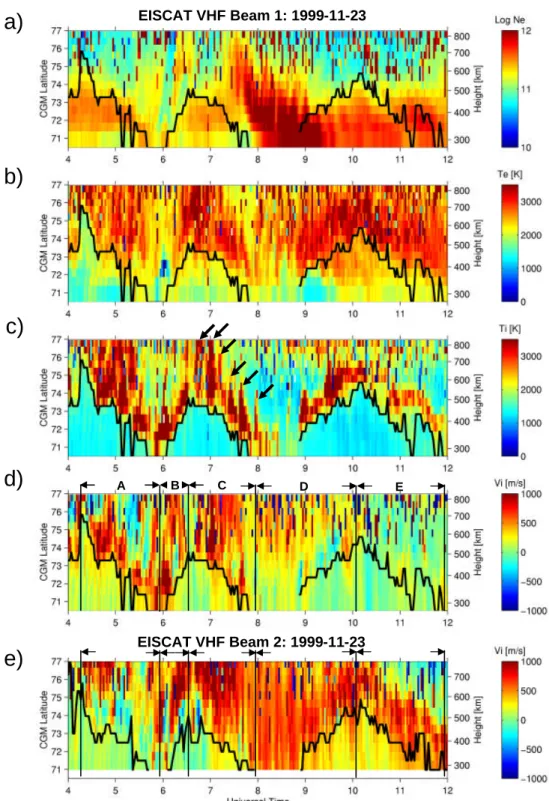
e)

Fig. 2. Plasma parameter plots obtained by EISCAT VHF in a V-shape configuration above Svalbard at 30◦elevation. Panels (a)–(d) show the electron density, electron temperature, ion temperature and line-of-sight ion velocity for the boresite Beam 1 pointing 15◦east of geographic north. The bottom panel (e) shows the line-of-sight ion velocity for the phase-shifted beam pointing towards geographic north. Positive velocity means away from the radar (poleward).

(CGM) latitude – observation time format. Note that, be-cause the beams are at 30◦ elevation, the height of the ob-servations varies from near 250 km at 70◦ latitude to near 800 km at 77◦ latitude. The data shown are: the electron concentration, Ne, in Fig. 2a; the electron temperature, Te,

in Fig. 2b; the ion temperature, Ti, in Fig. 2c; and the

line-of-sight (l-o-s) ion velocity, Vi, in Fig. 2d (Vi>0 is defined

as away from the radar). In order to ease the comparison be-tween Beam 1 and Beam 2, the l-o-s velocity from Beam 2 is presented in Fig. 2e. The other plasma parameters are almost identical to Beam 1 and are therefore not presented.

The azimuth angles for Beam 1 and Beam 2 were, re-spectively, 359.8◦_{and 344.8}◦_{east-of-north. The geometry is}

displayed in Fig. 3a, where the dotted curves represent con-stant CGM latitude (L-shells) from 66–86◦in 4-degree inter-vals. Beam 2 is directed towards the magnetic pole, while Beam 1 is pointing towards geographic north and makes an angle 15◦toward magnetic east with respect to Beam 2. The outstanding feature that drew our attention to the data presented in Fig. 2 is the narrow channel of enhanced Ti

zigzagging north-south over more than five degrees in mag-netic latitude, several times in the interval shown. The black curve superimposed on the upper four panels represents the Ti=1700 K iso-contour line extracted from the equatorward

edge of the high Ti band in Fig. 2c. The black contour

su-perimposed on the Beam 2 l-o-s velocities in Fig. 2e is the corresponding Ti=1700 K boundary derived for Beam 2.

Be-fore looking into more detailed plasma characteristics with emphasis on two DMSP satellite passes, we would like to describe the general flow picture observed as the radar pro-gressed in magnetic local time from near 07:00 to 15:00 MLT (MLT=UT+3 h) under a two-cell flow pattern. As the gov-erning IMF condition was BY positive and BZ negative, we

expect a two-cell flow pattern with a large afternoon cell and a crescent-shaped morning cell (Heppner and Maynard, 1987). A subdivision of the full period into five time inter-vals, A–E, are marked by vertical lines on Figs. 2d and 2e.

During interval A, from 04:20 to 06:00 UT, the Ti

chan-nel migrated equatorward. Beam 1, directed 15◦east of the magnetic meridian, experienced a strongly enhanced flow away from the radar (Vi>0) immediately poleward of the

Ti=1700 K boundary. When not interrupted by strong

pole-ward flows a prominent flow shear is situated within or near the poleward boundary of the high Ti band: poleward of this

shear Vi<0 (compare Figs. 2c and 2d). Beam 2 saw the same

flow shear, but with the polarities of Vireversed in that weak

toward flow was seen within the Ti channel and a large away

flow poleward of it. This is consistent with both beams look-ing eastward across a crescent-shaped convection dawn cell, as expected for the observed positive IMF BY. Beam 2,

ori-ented more closely to the magnetic meridian, picked up a relatively strong northward component of the anti-sunward flow, poleward of the CRB. The weak toward flow equator-ward of the CRB indicates that Beam 2 had a small westequator-ward tilt relative to the convection-reversal boundary. At the end of interval A, at around 05:40 UT, the convection reversal dis-appeared. Instead we see two prominent events of enhanced poleward flow. In Beam 1, the two events first appeared near the Ti boundary at 05:42 UT and 05:55 UT (Fig. 2d) and

pro-gressed poleward over the entire latitude range. In Beam 2, these onsets occurred a few minutes later, but are outstand-ingly clear at 05:46 UT and 06:00 UT. Both events appear associated with plasma density patches observed in Fig. 2a. These are signatures expected of reconnection pulses or “flux transfer events” (FTEs; Moen et al., 2001; Lockwood et al., 2001), indicating that the radar experienced plasma convect-ing away from the cusp region.

The Tiboundary retreated poleward immediately after the

onset of the second transient event and moved poleward until 06:35 UT (interval B). During interval C (06:35–08:00 UT), the Ti boundary migrated equatorward again to a location

to the south of the radar f-o-v. After 07:00 UT strong away flow is seen in both radar beams poleward of the Ti

bound-ary (black line) with weaker away flow equatorward of it. The away flow becomes gradually weaker in Beam 1 but is only slightly reduced in Beam 2, indicating that Beam 1 started to experience less longitudinal flow but the poleward flow is maintained as the radar f-o-v moves into the after-noon convection cell. In Fig. 2a we see that a “tongue” of enhanced ionization is being fed into the polar cap between 07:30 and 09:00 UT. This tongue exhibits poleward-moving fine structure which has been studied in greater detail by Davies et al. (2002), who show that it matches up closely with poleward-moving events seen simultaneously and in the same region in HF backscatter echoes observed by the CUT-LASS radar. The tongue of ionization seen in the electron density is another indicator that solar EUV ionized plasma drifted into the polar cap from the dusk sector. Some time after 08:00 UT (interval D) the polar-cap boundary retreated poleward once more, but the movement is not apparent in the ion temperature until Ti increased above the 1700 K

thresh-old set for boundary tracing at 08:55 UT. Notably, the ion temperature is low near the local noon at 08:50 UT. Strong away flows (0.5–1 km s−1)were maintained along the entire range of Beam 2. Around 09:00 UT Beam 1 started to see significant toward flow within the Ti channel, and a flow

re-versal near the poleward boundary of the Ti channel is

rela-tively well-defined between 09:10–09:45 UT, while Beam 2 is seeing strong away flow at all latitudes above the low-latitude edge of the Ti enhancement. This is consistent with

Beam 2 looking along convection streamlines flowing into the polar cap, while Beam 1 observes the CRB of the more circular dusk cell for IMF BY>0. Beam 2 also saw the

after-noon cell CRB from 10:30 UT onwards when it was absent in Beam 1 (period E, in which the boundary is expanding equatorward again).

In summary, the radar data are broadly consistent with the radar rotating, with the Earth under the form of the con-vection pattern expected for the IMF orientation that was observed to prevail throughout most of the interval studied (BY>0 and BZ<0). However, the pattern is far from steady

in form and the channel of enhanced Ti, in which the CRB

is embedded, is seen to migrate polewards and equatorwards over the radar field-of-view.

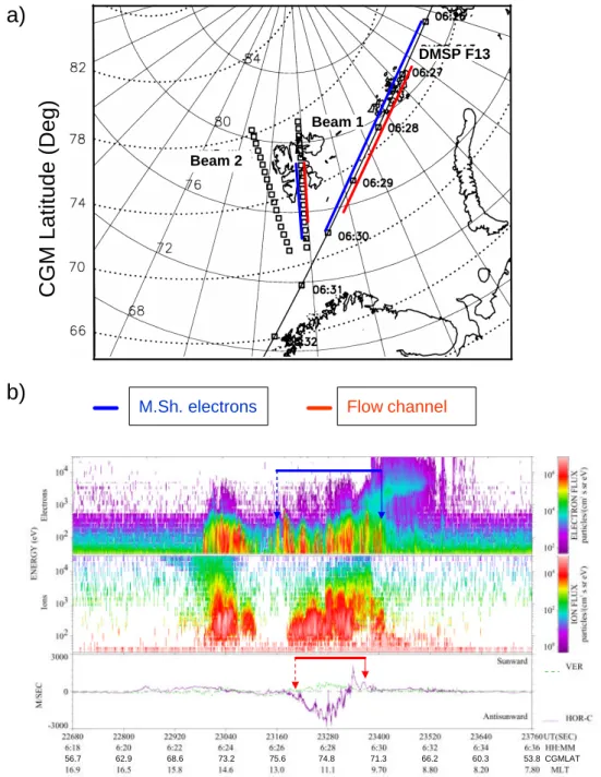
Against this background of the convection pattern and its variations, let us now have a detailed look at EISCAT bound-ary observations associated with two DMSP satellite passes close to the radar f-o-v. Figure 3a demonstrates the path of DMSP F13 as it passed to the east of the EISCAT VHF beams around 06:29 UT. The precipitating electron and ion fluxes measured along this path are presented in the upper two pan-els of Fig. 3b. DMSP F13 had two encounters of cusp-like precipitation, one centred on 06:24 UT (14:36 MLT), and the other one at 06:28 UT (11:06 MLT). It is the latter encounter

Figure 3

Map in

here

M.Sh. electrons Flow channel

b)

CGM Latitude (Deg)

a)

Fig. 3. (a) The geometry of the DMSP F13 pass east of EISCAT’s Beam 1 and Beam 2 around 06:30 UT. The blue bar along the satellite trajectory marks the spatial extent of magnetosheath electron precipitation, and the red bar marks the extent of a convection flow channel observed by the satellite. These bars have been mapped along the L-shells onto Beam 1 and will be compared with electron and ion gas temperatures measured by EISCAT. (b) Electron and ion precipitation fluxes and cross-track (magenta) and vertical (green) flows measured by the drift meter on board DMSP. The blue bar corresponds to the blue bars in (a), and the solid arrow (dashed arrow) marks the equatorward (poleward) edge of intense magnetsheath-like electron precipitation. The red bar and arrows mark out the convection channel to be compared with enhanced EISCAT Ti measurements.

of cusp precipitation that is of particular interest for com-parison with EISCAT because it is close to the radar f-o-v. We would like to check whether the high Ti band is related

to a flow channel, and we would also like to see if the edge of magnetosheath electron precipitation is associated with a well-defined boundary of enhanced Te. Based on two

satel-lite passes it is of course not possible to establish a quantita-tive approach for this comparison. However, the equatorward edge of magnetosheath electron precipitation is rather well defined. In Fig. 3b the equatorward edge is marked by a blue arrow, and the poleward edge is indicated by a dashed blue arrow. These two arrows are connected with a blue bar which

Figure 4

Fig. 4. The Te(red curve) and Ti(blue curve) versus altitude along Beam 1 for data integration periods commencing at 06:28 and 06:30 UT.

The blue and the red bars are corresponding to Fig. 3 and mark out the regions of magnetosheath electron precipitation and the plasma flow channel measured by DMSP F13. The flow reversal boundary is indicated by the black arrow. The horizontal dashed line is a guideline for the Ti=1700 K boundary.

has been transferred to the satellite trajectory in Fig. 3a, and mapped along the magnetic L-shells onto VHF Beam 1. The satellite trajectory and the radar gate positions have been transformed to the Corrected GeoMagnetic (CGM) coordi-nates. Figure 4 presents ion temperature (red) and electron temperature (blue) observed along radar Beam 1. The varia-tion is a funcvaria-tion of range, which mixes altitudinal and lati-tudinal variations. In the vertical axes of Fig. 4 we use height to remind us that this is also a relevant factor. Figure 4 shows data from two successive 2-min data integration periods com-mencing at 06:28 UT and 06:30 UT. The latitudinal variation in both temperatures is superposed as an upward trend that is caused by the increase in altitude of the beam. This alti-tude effect will be greater for the electron temperature. How-ever, we can note that the equatorward boundary of the low-energy electron precipitation is related to a significant gradi-ent in the electron temperature on the 06:28 UT profile. In the 06:30 UT profile a significant Te-gradient was observed two

range gates further north, i.e. at range gate 4 around 390 km altitude. In the bottom panel of Fig. 3b we see that the cusp precipitation east of EISCAT Beam 1 was associated with strongly enhanced cross flow. The horizontal cross-track component is indicated in magenta (positive sunward), and the vertical drift is plotted in green (positive up). Horizontal flow speeds of up to 2 km s−1 are observed. Since we have chosen 1700 K to delineate the equatorward boundary of the Joule-heating channel, it would be interesting to see what it

corresponds to in terms of DMSP flow data. From the Ti

curve in Fig. 4 we see that the 1700 K boundary corresponds to the red arrow at 390 km altitude (gate 4). Mapped onto the satellite track this corresponds to the right-hand red arrow placed at 06:29:30 UT which points out a local maximum in the return flow of 0.9 km s−1. The left-hand red arrow rep-resents the 0.9 km s−1 threshold at the poleward boundary near 06:26:15 UT. Mapped backwards onto the radar beam this correspond to 680 km just poleward of gate 11. Between 06:26 and 06:27 the satellite nearly skimmed the L-shell and hence, the poleward boundary of the flow channel and the poleward boundary of the magnetosheath electron precipita-tion map to almost the same posiprecipita-tion along the radar beam. In the discussion we will focus on the equatorward bound-aries only since the poleward boundbound-aries (dashed arrows) are involved with large uncertainties. However, it is worthwhile to notice that the CRB is embedded in the flow channel/ high Tiand that the sense of flow geometry is consistent with what

we postulated based on the EISCAT observations. In Fig. 4 the flow reversal is indicated by the black arrow.

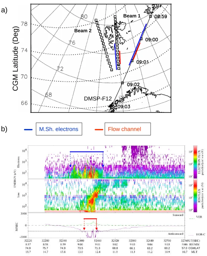
DMSP F12 passed along a similar trajectory 2.5 h later, around 09:01 UT, as depicted in Fig. 5a. The observations made during this pass are presented in Fig. 5b. The F12 satel-lite traversed a well-defined electron edge near 09:01:20 UT, although precipitating fluxes of magnetospheric electrons were weak immediately poleward of that edge. The ion data show a stepped ion dispersion signature with its high-energy

Map to

come

M.Sh. electrons

Flow channel

Figure 5

b)

a)

DMSP-F12

CGM Latitude (Deg)

Beam 2

Beam 1

Fig. 5. Similar presentation as in Fig. 3 but for the DMSP F12 pass at around 09:00 UT.

edge located poleward of the magnetosheath electron edge. As in the previous example, the band of magnetosheath elec-tron precipitation has been projected along L-shells onto the EISCAT VHF Beam 1 in Fig. 5a. Figure 6 presents Ti (red curve) and Te (blue curve) along the beam (as for

Fig. 4, shown as a function of height) for the data integra-tions commencing at 09:00:00 UT and 09:01:59 UT. Temper-atures above 4000 K are bad fits. Steep gradients are seen in both Teand Ti, and these are contracting poleward with time

Figure 6

Fig. 6. The Teand Tiversus height along EISCAT Beam 1 for 09:00 and 09:01:59 UT data records.

DMSP F12 09:00 UT Cusp/Cleft Flow channel Reconnecting OCB Non-reconnecting OCB DMSP F13 06:30 UT a) b) Figure 7

Fig. 7. Diagrams summarizing the information derived from the two satellite passes. Notably, the flow-reversal boundary observed on the prenoon sector of the F13 pass was located ∼300 km pole-ward of the open-closed field-line boundary, which is evidence of sunward return flow along open field lines.

the equatorward limit of the f-o-v, but Te seems to be

sensi-tive to even modest fluxes of magnetosheath electrons. As-sociated with the cusp crossing, DMSP observed two bursts of strongly enhanced flows peaking above 3 km s−1. The Ti=1700 K boundary near gate 2 corresponds to the

equa-torward edge of the strong flow disturbance which appear superimposed onto a background flow of ∼1.4 km s−1 anti-sunward. We tentatively define the flow channel/Joule heat-ing region to include both high speed streams. Mappheat-ing the poleward boundary (dashed arrow) back to EISCAT Beam 1 it corresponds to gate 6, poleward of which there is a signifi-cant decrease in Ti.

3 Discussion

The flow and precipitation patterns that are inferred from the snapshots provided by the two DMSP passes are schemati-cally summarised in Fig. 7. The red bar is consistent with the band of high Ti, as seen by EISCAT at these times, and the

schematics are consistent with the inference from the EIS-CAT velocity data that the CRB is within the high-Ti band

for both beams at 06:30 UT and for Beam 2 at 09:00 UT, but that the CRB is at the equatorward edge of the high-Ti band

at 09:00 UT for Beam 1. For the IMF orientation (with BY>0

and BZ<0) the CRB is most apparent in the dawn cell, and

we conclude that both beams were observing the dawn cell at 06:30 UT, and around 09:00 UT Beam 2 was situated in the dawn cell, whereas Beam 1 was situated in the dusk cell.

As illustrated in Fig. 7a, DMSP F13 first encountered magnetosheath precipitation (blue bar) with weak cross-track drift in the ∼14:00–15:00 MLT sector. The DMSP satel-lites carry a Retarding Potential Analyser (RPA) to measure along-track plasma speed. In this case the data quality was poor, and the only information we have about convection is the lack of significant cross-track flow, indicating that the satellite path was close to being aligned with the convec-tion streamlines. After a brief excursion poleward of the cusp, it traversed the cusp precipitation region for a second time, this time in the 10:00–12:00 MLT sector. This indicates that the width of the cusp was at least five hours in MLT at this time. The very strong anti-sunward flow observed dur-ing the prenoon cusp encounter (2–3 km s−1)and the lack of a clear ion dispersion signature (cf. Fig. 3b) is consistent

with the satellite path in the second cusp intersection being almost perpendicular to the flow streamlines (so the along-track flow component must have been small here). The band of cusp precipitation extends on either side of the convec-tion channel (>1 km s−1)marked in red. It is particularly interesting to see such clear evidence of sunward flow on field lines showing cusp particle precipitation, equatorward of CRB but poleward of the magnetosheath electron edge. The flow-reversal boundary is 2.7◦(300 km) poleward of the electron edge, which is taken to be an indicator of the open-closed field-line boundary (Sandholt et al., 2002). The elec-tron edge appears to coincide with elevated Te in magnetic

latitude, while the Ti=1700 K boundary (equatorward edge

of the flow channel) was located 1.2◦(130 km) poleward of the electron edge.

The DMSP F12 pass illustrated in Fig. 7b made more like a meridional cut through cusp precipitation in the postnoon sector where it observed a strong cross-track flow. In this case we see prominent ion dispersion and steps in the ion en-ergy cutoff. The Ti gradient observed by EISCAT coincided

with the equatorward edge of strongly enhanced ion convec-tion (Fig. 6). In this case the electron edge was corresponding to the southernmost radar gate, which makes it impossible to define a temperature boundary. However, the sharp gradient in Te between gate 1 and 2 (300 K over 36 km altitude

dif-ference) indicates a significant heating due to the low energy electron precipitation.

We are going to conclude that the Ti=1700 K isocontour

boundary represents a proxy for the polar-cap boundary, and in Sect. 3.1 we will relate the north-south zigzagging mo-tion of that boundary to unbalanced dayside and nightside reconnection. Section 3.2 is devoted to a physical explana-tion for the prominent Tichannel that lasted several hours in

the EISCAT f-o-v. In Sect. 3.3 we look more closely at the DMSP precipitation characteristics with respect to the open-closed field-line boundary, and discuss the potential of us-ing Te versus Ti gradients as a proxy for the open-closed

field-line boundary. We are going to conclude that the Ti

-boundary represents a proper reference for calculating the reconnection rate.

3.1 Dayside polar-cap boundary movement versus IMF BZ

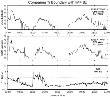
Figure 8 presents the Ti=1700 K isocontour boundary on the

equatorward edge of the high Ti band, for EISCAT Beam 1

and Beam 2 (upper and middle panels, respectively), along with variations in IMF BZ (bottom panel). The time axis

for the IMF BZ variation has been shifted by one hour with

respect to the Ti-plots to adjust the time lag between ACE

located 230 REupstream and the ionospheric response. This

lag is calculated from the observed solar wind speed and, as discussed below, allows for various features observed by EISCAT to be matched up with causal IMF features. Up to about 08:00 UT, the latitudinal movements of the Ti

bound-ary appear closely related to changes in IMF BZ. From

03:00 UT to 05:00 UT ACE observed a gradual decrease in BZfrom 0 to −7.5 nT, giving rise to enhanced magnetopause

04:00 05:00 06:00 07:00 08:00 09:00 10:00 11:00 12:00 71 72 73 74 75 76 77 CGM Latitude EISCAT VHF CP4 North Ti=1700K Comparing Ti Boundary with IMF Bz

71 72 73 74 75 76 77 CGM Latitude EISCAT VHF CP4 West Ti=1700K −10 −5 0 5 10 nT [GSM] ACE IMF Bz 03:00 04:00 05:00 06:00 07:00 08:00 09:00 10:00 11:00 Universal Time

Fig. 8. The upper two panels show the Ti=1700 K isocontour

boundary derived from EISCAT Beam 1 and Beam 2, and the bot-tom panel shows IMF BZobserved by ACE. Note that the ACE time

scale is shifted by one hour relative to the EISCAT observations.

reconnection seen by the radar as an expansion of the po-lar cap from 04:00 to 06:00 UT. The sharp northward turn-ing observed by ACE at 05:00 UT effectively stopped the production of new open flux. The poleward contraction of the polar cap from 06:00 and 06:40 UT appears consistent with the closure of flux by lobe reconnection on the day-side lobes. However, around the same time at 06:00 UT, a negative bay in the AL index peaked at −460 nT (not pre-sented), and a much more likely explanation is a closure of flux by reconnection in the cross-tail current sheet. In this case, as IMF |BY|dominated IMF |BZ|after the northward

turning, lobe reconnection is expected to stir open flux oppo-sitely in the two hemispheres rather than giving rise to clo-sure of flux. Looking at the more-detailed structure in the response, it is interesting to note that the negative deflection in IMF BZ observed by ACE between 05:40 and 05:50 UT

lines up perfectly with the brief equatorward bounce in the Tiboundary in Beam 2 between 06:40–05:50 UT. If real, this

boundary movement must have been local, as it was not evi-dent in Beam 1. More significant, however, is the subsequent rapid decrease in BZfrom near zero to −7 nT from ∼05:50

to 06:00 UT (at ACE), after which the IMF BZ stayed

neg-ative throughout the time interval considered in this study. Enhanced magnetopause reconnection and efficient opening of flux migrated the Ti boundary more than four degrees

in latitude out of the radar f-o-v. When the boundary be-came detectable again at 08:50 UT, a rapid poleward retreat was observed until 10:15 UT. This can only be explained by tail reconnection and closure of flux. Between 08:08 UT and 08:28 UT the AL index dropped from −160 to −990 nT, indi-cating strong tail reconnection. Based on the Dungey (1961)

reconnection model, it has become well established that if the magnetopause reconnection rate exceeds the reconnection rate in the geomagnetic tail, the polar cap expands. Likewise, if the nightside reconnection rate exceeds that of the day-side, the polar cap size decreases. Siscoe and Huang (1985) established a model for how polar-cap boundary movement due to unbalanced dayside and nightside reconnection gives rise to excitation of large-scale polar cap convection. Cow-ley and Lockwood (1992) further refined a conceptual model to explain the impact of unbalanced, time-dependent recon-nection on the generation of large-scale polar cap convec-tion. Lockwood et al. (1988), Lester et al. (1990) and Fox et al. (1994) documented large-scale displacements of the polar-cap boundary in the 04:00–10:00 MLT sector, found expansion of the polar cap consistent with magnetopause re-connection, and ascribed contractions of the polar cap to sub-storm activity. In the case presented by Lester et al. (1990), the contraction occurred despite the fact that the IMF was strongly southward (BZ near −10 nT). Milan et al. (2003)

conducted a comprehensive study, including a global survey by the Polar Ultraviolet Imager (UVI) and SuperDARN HF radar, observing variations in the polar cap area as a func-tion of changing IMF and substorm activity. In the time in-terval presented by Milan et al. (2003), IMF BZ was

fluc-tuating between positive and negative values, and the major polar cap contraction event occurred during IMF BZ north.

The case presented in Fig. 8 provides a new example of this effect under different IMF conditions, where unbalanced re-connection dominated by tail gave rise to a rapid poleward contraction in the 12:00–13:00 MLT sector when IMF BZ

stayed strongly negative.

3.2 Ionospheric flow and plasma dynamics associated with the high Tichannel

The band of high Ti was observed to be a

persis-tent feature from 04:15 UT (∼07:25 MLT) until 12:00 UT (∼15:10 MLT), except for a half-hour break near magnetic noon at around 08:50 UT. This is taken as an indicative that the Tichannel was extended along most of the dayside

auro-ral oval, and persistent in time. The latitudinal width of the Ti

band varied spontaneously from 1◦to 4◦CGM Lat. The vari-ation in width was particularly strong during intervals A and C when the Tiboundary migrated equatorward. Ti

enhance-ments appear modulated by corresponding enhanceenhance-ments in the line-of-sight flow velocity. For example, during interval C, a sequence of six Tievents is marked by arrows in Fig. 2c,

and these seem all to be associated with a flow enhancement in Fig. 2d. The first five events were associated with bursts in the poleward flow, while the later event (near 08:00 UT) coincided with toward flow in Beam 1 but poleward flow in Beam 2 (Fig. 2e).

The combination of EISCAT Ti and DMSP F12 and F13

flow observations addresses the Ti=1700 K boundary to the

equatorward edge of a strong flow disturbance (Figs. 3–6). F12 and F13 were, respectively, separated 1 and 2.5 h in magnetic local time east of the EISCAT f-o-v when they

in-tersected the poleward edge of the flow channel. Further-more, the signal-to-noise ratio of the radar pulse decreases with range, and the data quality becomes poorer at higher latitudes. Because of these uncertainties we will not focus on the observations near the poleward edge. However, the latitudinal width of the flow channel intersected by the two DMSP passes was about two degrees in latitude.

Pinnock et al. (1993) reported on a zonally-aligned narrow channel of enhanced convection, at least 900 km in longitu-dinal extent and 100 km wide. On the basis of combined data from the PACE HF radar in Antarctica, DMSP particle and drift meter, they located the flow channel to the equator-ward part of the cusp precipitation region. They attributed flow bursts on the order of 3 km s−1 within this channel to candidate flux transfer events (FTEs). EISCAT observations of strong plasma flows in the auroral cusp were reported by Lockwood et al. (1990), and the phenomenon of latitudinally confined strong flows in the cusp has been reported by e.g. Valladares et al. (1994, 1999) and Pinnock et al. (1991).

Narrow zones of frictional heating may occur near the day-side and the nightday-side part of the auroral oval (Lockwood et al., 1988; Woodfield et al., 2002). The ion heating rate is proportional to the square of the ion-neutral gas velocity dif-ference, and for relative velocities more than a km s−1, the ion temperature is enhanced by over ∼1000 K. This is what produces the hot ion channel. According to model results by Lockwood and Fuller-Rowell (1987a, b), if the neutral wind pattern had reached a diurnal equilibrium prior to ex-pansion (contraction) of the polar cap, there will form a band of strong frictional heating immediately poleward (equator-ward) of the expanding (contracting) flow-reversal boundary. This is because ion flow on the trailing edge of a moving convection boundary will meet neutral wind which has yet to respond to the change. Examples of this effect were demon-strated by Lockwood et al. (1988) and Fox et al. (1994). However, these examples were away from noon and required a strong shear CRB. This idea is not consistent with the near-noon observations presented here except maybe for interval D (from 09:15–09:45 UT), where high Ti was located

equa-torward of the flow-reversal boundary as it retreated pole-ward (Figs. 2c and 2d). During the expansion in interval A, the band of high Ti region is located mainly equatorward of

the flow-reversal boundary, or is sometimes straddling the flow-reversal boundary along the two radar beams (Figs. 2c– 2e), while according to the “trailing-edge” concept Joule heating should occur poleward of the flow-reversal bound-ary. For the F13 pass around 06:30 UT, high Ti spanned the

flow-reversal boundary, with large ion flows on either side (Figs. 3 and 4). During interval C, the Ti band is not related

to a flow-reversal boundary at all, but rather to a prominent acceleration in the poleward flow. The DMSP pass around 09:00 UT did not observe any flow shear, but instead a chan-nel of strongly-enhanced anti-sunward flow (north-westerly oriented) in association with the Ti-band. The 5–10 min.

modulation of Tiis probably caused by pulsations in the

con-vection electric field applied on the ionosphere, rather than the potential role of retarding ion and neutral flows. The fact

that the polar-cap boundary was rapidly zigzagging in lat-itude means that it was unlikely that the near-noon neutral winds built up to a strong and steady pattern, which was a required condition for the model results by Lockwood and Fuller-Rowell (1987a, b).

The narrow gap in the Ti channel near magnetic noon

(between about 08:25 and 08:50 UT) indicates that the cusp trough has covered this MLT sector sufficiently long that the neutral wind has been speeded up to the same magnitude as the ion flow. Note that at 250 km, the mean time for an ion to collide with a neutral particle is about a second; near 300 km, a few seconds (e.g. Banks and Kockarts, 1973). If the ion gas is at rest in the neutral gas rest frame (no relative velocity of one with respect to the other), the ion temperature will come into equilibrium with the neutral gas temperature within a few collision times. If the ion gas is moving relative to the neutral gas, an ion colliding with a neutral will suffer tion of some of its ordered motion, and this random redirec-tion is ion heating. Now consider the time for the neutral gas to respond to ion gas moving through it and compare with the time of about a second for the ion gas to respond to col-lisions with the neutrals in which it is immersed. The mean time for a neutral particle to collide with an ion is longer than the mean time for an ion to collide with a neutral, by the ratio of the number of neutral particles per unit volume to the number of ions. At around 250–300 km, the number density of atomic oxygen is near 1015m−3, compared with the 1012m−3ion density in the Ti gap region. Thus, it takes

about 1000 times longer for the neutrals to respond than the ions, i.e. ∼1000 s. The nature of the response to a persistent ion flow is that a neutral particle continues with the initial ion velocity, and the ion starts life with the neutral particle velocity. This is because collisions are via a charge transfer reaction: an electron transfers from a neutral atomic oxygen particle to an atomic oxygen ion, and then they exchange roles. Thus, within about half an hour (a couple of collision times) the neutrals are up to speed with the plasma flow, for the 1012m−3 ion density near local noon, where the high-density plasma flow is entering the polar cap. This can only occur provided that high plasma density and enhanced flow persist for that long. The high-density plasma channel is well over an hour in width. The IMF orientation was stable from 06:00 UT onwards, corresponding to 07:00 UT onwards in the ionosphere, suggesting that the MLT location of the cusp inflow region might well have been stable for an extended time around the observed gap in high Ti. Consequently, ion

heating is absent (negligible relative velocity), and in addi-tion, a huge channel of thermospheric flow is directed into the polar cap. At UTs prior to the high ion density cusp sec-tor, the ion densities are only a few times 1011m−3, and the neutrals would take hours to come up to speed, time they do not have. In going from an ion density of 1012m3to one of 1011m−3, the collision time goes from of the order of half an hour to of the order one quarter of a day. Thus, the ions in the sunward flow region meet a thermosphere nearly at rest. With a response time of the ion-neutral collision time of ∼1 s, the ion gas comes to a high equilibrium temperature

con-trolled by strong ion winds. Likewise, post-magnetic noon, the ion densities fall sufficiently that the neutral-ion colli-sion time exceeds the time a nominally co-rotating part of the thermosphere experiences a nominally constant plasma flow velocity vector, and again, the ion heating is controlled by high speed ions.

Cowley et al. (1991) discussed high-speed plasma flows immediately poleward of the open-closed field-line bound-ary in terms of the tension force on newly-opened magnetic field lines. Given that the high Ti is a signature of

newly-open flux, it should be pointed out that the eight hours of continuous observation of high Ti does naturally not imply

that the longitudinal width of the cusp was eight hours at any one time. The ionospheric cusp reconfigures in response to changes in IMF within minutes (Moen et al., 1999, 2001). However, from the DMSP F13 we know that the cusp was at least five hours wide around 06:30 UT. Doe et al. (2001) reported a band of high Telasting for six hours observed by

the Søndre Strømfjord radar. Milan et al. (2000) and Moen et al. (2001) observed moving cusp auroral signatures in the 16:00–17:00 MLT sector. So, cusp/open LLBL activity may occur in a wider span of local times than expected from the statistical survey provided by Newell and Meng (1992). 3.3 Ionospheric signatures of the open-closed field-line

boundary

At 06:30 UT, DMSP F13 crossed a region of mixed magne-tosheath and magnetospheric electrons prior to encountering the central plasma sheet (CPS). The region of mixed elec-tron particle fluxes located on sunward return flow is a can-didate low-altitude signature of the mixing layer reported by Fujimoto et al. (1998). They observed a thin mixing layer associated with sunward flow on the dawn flank (06:00– 09:00 MLT). It was situated between the central plasma sheet and the convection-reversal boundary, and was tentatively at-tributed to closed LLBL.

On both sides of the convection-reversal boundary in Fig. 3, there is a weak flux of 3–20 keV ions on the top of the intense flux of low-energy magnetosheath ions. Lock-wood and Moen (1996) explained the mixture of magneto-spheric and magnetosheath ions by introducing a reconnec-tion model that includes interior and exterior rotareconnec-tional dis-continuities (Alfv´en waves) emanating from the reconnec-tion line. Their model results showed that magnetospheric ions can be injected on open LLBL field lines by reflection of the pre-existing magnetosphere by the interior Alfv´en wave. The mixing of magnetospheric and magnetosheath electrons is not well understood. The poleward boundary of high-energy electrons has traditionally been taken as a marker of the open-closed field-line boundary, as magnetospheric electrons on newly-open field lines are expected to escape within one-quarter of a bouncing period, i.e. within sec-onds. Oksavik et al. (2000) demonstrated an ambiguity prob-lem by applying the above rule of thumb for identifying the open-closed boundary. An isotropic flux of energetic elec-trons was observed on field-line-associated magnetosheath

particle injection and a staircase ion-dispersion signature. The staircase ion cusp and poleward moving auroral forms are regarded as key signatures of transient magnetopause re-connection (Newell and Meng, 1991, 1995; Lockwood and Smith, 1992; Onsager et al., 1993; Farrugia et al., 1998; Lockwood and Davis, 1995; Lockwood et al., 1998), while energetic electrons are used as a tracer of closed flux.

Lockwood (1998) put forward a possible explanation for a mixing layer on sunward convection immediately pole-ward of the opclosed field-line boundary, which is en-tirely consistent with the observations presented here. The flow-reversal boundary marks out the location where the in-terior Alfv´en wave arrived. It may take several Alfv´en wave bounces until sufficient momentum has been carried down to change the direction of the ionospheric flow from sunward to antisunward, i.e. the newly-open flux continues to stream sunward several minutes after being opened. Super-Alfv´enic sheath particles (electrons and the more energetic ions) will arrive before any change in the flow and the CRB may not be complete until several bounces of the interior Alfv´en wave. Notable from Fig. 3b is that the energetic electron popula-tion bordered on the prenoon LLBL but not on the postnoon LLBL/Cusp. The CPS population tails off within the mix-ing layer, which indicates that rmix-ing current electrons have penetrated the LLBL boundary by gradient-B and curvature-B drifts, which are breakdowns of the frozen-in approxima-tion. Interestingly, the highest energy of this population de-creases with increasing latitude, which means that the high-est energies are emptied first. Gradient-B and curvature-B drifts of electrons onto newly-opened field lines may con-tinue as long as a contact surface exists between the open and closed fluxes. It has also been postulated that magneto-spheric particle fluxes can be maintained by magnetic bottles on open field lines, as the field strength has a minimum at middle latitudes in the magnetic cusp (Cowley and Lewis, 1990; Scholer et al., 1982; Daly and Fritz, 1982). Nishida et al. (1993) reported open-flux characteristics on sunward re-turn flow. According to Lockwood (1998) the mixing layer is on open field lines, located between the central plasma sheet and the flow-reversal boundary.

From the observations presented here, it is possible to dis-cuss the general location of the reconnection site. Earlier in Sect. 3, we noted that DMSP F13 observed the CRB and the equatorward edge of the high flow band (Ti=1700 K) to

be, respectively, 2.7◦and 1.2◦poleward of the electron edge, which is taken to be an indicator of the OCB. These latitude differences correspond to northward distance dn of 300 and

130 km. Because of the lack of a strong ion dispersion sig-nature, we can assume that the along track convection com-ponent is small, so the flow speed Vcis similar to the

cross-track component (of the order of 1 km s−1). From this, the northward component of the flow Vcn is about 0.5 km s−1

(a similar value is derived in this region using the EISCAT line-of-sight velocities). If we take the equatorward edge of the high flow/high-Ti band to be where the flow begins to

change because of the arrival of the interior Alfv´en wave, this means that the wave took 260 s longer to reach the

iono-sphere than the first electrons. We see sheath electrons at all energies down to 30 eV at this edge (a field-aligned speed of Ve=3200 km s−1)and we here assume the Alfv´en wave

to travel at an average speed of VA=1000 km s−1. The

dif-ference in travel times of the wave and the edge electrons is (1tA −1te)=d(V_A−1−V−e1), where d is the field-aligned

distance to the reconnection site. For a poleward convection speed Vcn, this time difference corresponds to a latitudinal

distance dn=(dA−de)=Vcn(1tA−1te). Thus,

d = (dn/Vcn)/(V−_A1−V−_e1). (1)

Substituting the above values into Eq. (1) yields d of ∼60 RE,

that the electron edge is de=60 km poleward of the actual

magnetic footprint of the X-line, and the arrival of the wave is dA=190 km poleward of the OCB. Note that a reflected

“second-bounce” Alfv´en wave would return to the iono-sphere after about 31tAafter reflection from the (open)

mag-netopause and so would be at least three times this distance from the OCB. Thus, such an effect is not an explanation of the CRB which is here estimated to be 360 km from the OCB. The large d derived clearly indicates a reconnection site on the flank of the magnetosphere.

The two DMSP snapshots indicated a relationship between elevated Te near the equatorward edge of magnetosheath

electron precipitation, which is consistent with earlier work (cf. Introduction). However, one should exercise caution when employing Teas a marker for precipitation boundaries,

in particular for the geometry of the EISCAT CP-4 experi-ment when we do not have altitude profiles. Carlson (1998) pointed out that the cooling rate of electrons is proportional to the square of the electron density, and for electron den-sities much above 3×1011m−3, the electron gas is in good thermal contact with the ion gas. Based on the energy equa-tion from Banks and Kockarts (1973), Doe et al. (2001) demonstrated that electron cooling may suppress the Te

sig-nature below 400 km. We do see an example of this in the present data set, where we see “bite-outs” in the high elec-tron temperatures associated with the tongue of ionization. After about 09:20 we see another complexity, that is, the el-evation of Te due to sunrise and solar illumination, and the

Te boundary fails for this reason to be a simple boundary

marker.

In general, Tecan serve as a simple particle-precipitation

boundary marker when other electron gas heating terms are absent, and electron cooling rates are modest (ion densities near and below about 3×1011m−3). For other conditions, more careful analysis of the thermal balance is needed to draw conclusions about boundaries.

4 Summary and concluding remarks

The narrow channel of Joule heating indicates that the trans-fer of momentum from the solar wind to the ionosphere takes place in a latitudinally confined region. This has earlier been reported as a cusp phenomenon, but the near to eight-hour continuous observation by the EISCAT VHF radar on 23

November 1999 is quite unusual, and gave us a unique op-portunity to test ionospheric electron and ion temperature gradients as markers for the open-closed field-line boundary. The north-south zigzagging was found to be entirely consis-tent with the Cowley-Lockwood model of unbalanced day-side and nightday-side reconnection rates. This data set provides a first experimental evidence of a rapid poleward contraction of the noon polar cap boundary under IMF Bz south

condi-tions.

The ionospheric electron temperature is sensitive to the precipitation of magnetosheath electron fluxes, as earlier demonstrated by the Søndre-Strømfjord and EISCAT Radar data and by modelling. The equatorward boundary of high Te

may sometimes serve as the initial marker of newly-opened flux. However, Te may fail as an open-closed boundary

marker in cases when: 1) the electron density is significantly above 3×1011m−3 _{(Carlson et al., 1998) (the T}

e boundary

is then generally suppressed at altitudes below ∼400 km, cf. Doe et al., 2001); 2) the electron plasma is heated by solar il-lumination; 3) the electron plasma is heated by high ion tem-peratures; and 4) the electron plasma is heated by downward heat conduction from a large heat reservoir in the flux tube above the F-region, as for a currently or previously closed magnetic flux tube that has not had time to cool. Note that L

∼6 flux tubes can take hours to cool down after both feet of the flux tube are no longer sunlit, at which time photoelec-tron heating of the ambient elecphotoelec-tron gas within the tube turns off. Due to changing conditions for thermal balance during the interval of interest here, we did not succeed with using Teas a tracker the open-closed boundary. A major limitation

for the EISCAT VHF convection experiment in this context is the lack of altitude profiles.

We conclude that the equatorward edge of the high Ti

channel manifests the arrival of the rotational discontinuity. The gap between the equatorward Tiboundary and the

equa-torward edge of magnetosheath electron edge was ∼60 km near 12:00 MLT (DMSP F12) and 130 km near 10:00 MLT (DMSP F13). The distance between the arrival of the first (super-Alfv´enic) magnetosheath electrons and the transfer of momentum carried by Alfv´en waves will naturally depend on magnetic field line distance between the magnetopause X-line and the ionospheric counterpart, as well as the con-vection speed at the ionospheric end. In general, this dis-tance will increase away from magnetic noon. In cases when release of magnetic tension gives rise to significant Joule heating, the equatorward Ti boundary is the actual reference

boundary to be used for calculating the reconnection rate. This will be treated in a separate publication by Lockwood et al. (2003).

The region of mixed magnetosheath and magnetospheric electrons between the convection reversal boundary and the electron edge, on sunward convecting flux, is a candidate footprint of the low-latitude boundary mixing layer on open field lines.

Acknowledgements. EISCAT is an international association sup-ported by Finland (SA), France (CNRS), the Federal Republic of Germany (MPG), Japan (NIPR), Norway (NFR), Sweden (NFR), and the United Kingdom (PPARC). We thank the ACE Science Cen-ter and the ACE MAG and SWEPAM instrument teams for provid-ing solar wind data from the ACE spacecraft. The work has re-ceived financial support from the Norwegian Research Council and AFOSR task 2311AS.

References

Banks, P. M. and Kockarts, G.: Aeronomy, Academic Press, New York, 1973.

Brace, L. H., Theis, R. F., and Hoegy, W. R.: A global view of the F-region electron density and temperature at solar maximum, Geophys. Res. Lett., 9, 989–992, 1982.

Carlson, H. C.: Response of the polar cap ionosphere to changes in (solar wind) IMF, Polar-cap boundary Phenomena, by Moen, J., Egeland, A., and Lockwood, M. (eds.) NATO Advanced Study Institute Series, Kluwer Academic Press, Dordrect, Vol. 509, 255–270, 1998.

Cowley, S. W. H. and Lewis, Z. V.: Magnetic trapping of ener-getic particles on open dayside boundary layer flux tubes, Planet. Space Sci., 38, 1343–1350, 1990.

Cowley, S. W. H., Morelli, J. P., and Lockwood, M.: Dependence of convective flows and particle precipitation in the high-latitude dayside ionosphere on the X and Y components of the interplan-etary magnetic field, J. Geophys. Res., 96, 5557–5564, 1991. Cowley, S. W. H. and Lockwood, M.: Excitation and decay of

so-lar wind-driven flows in the magnetosphere-ionosphere system, Ann. Geophys., 10, 103–115, 1992.

Curtis, S. A., Hoegy, W. R., Brace, L. H. et al.: DE-2 cusp observa-tions: role of plasma instabilities in topside ionospheric heating and density fluctuations, Geophys. Res. Lett., 9, 997–1000, 1982. Daly, P. W. and Fritz, T. A.: Trapped electron distributions on open

field lines, J. Geophys. Res., 87, 6081–6088, 1982.

Davies, J. A., Yeoman, T. K., Rae, I. R., Milan, S. E., Lester, M., Lockwood, M., and McWilliams, A.: Ground-based observa-tions of the auroral zone and polar cap ionospheric responses to dayside transient reconnection, Ann. Geophys., 20, 781–794, 2002.

Davis, C. J. and Lockwood, M.: Predicted signatures of pulsed re-connection in ESR data, Ann. Geophys., 14, 1246–1256, 1996. Doe, R. A., Kelly, J. D., and S´anchez, E. R.: Observations of

per-sistent dayside F-region electron temperature enhancements as-sociated with soft magnetosheathlike precipitation, J. Geophys. Res., 106, 3615–3630, 2001.

Dungey, J. W.: Interplanetary magnetic field and the auroral zones, Phys. Rev. Lett., 6, 47 –48, 1961.

Farrugia, C. J., Sandholt, P. E., Denig, W. F., and Torbert, R.: Ob-servation of a correspondence between poleward-moving auroral forms and stepped cusp ion precipitation, J. Geophys. Res., 103, 9309–9315, 1998.

Fox, N. J., Lockwood, M., Cowley, S. W. H., Freeman, M. P., Friis-Christensen, E., Milling, D. K., Pinnock, M., and Reeves, G. D.: EISCAT observations of unusual flows in the morning sector associated with weak substorm activity, Ann. Geophys., 12, 541– 553, 1994.

Fujimoto, M., Mukai, T., Kwano, H., Nakamura, M., Nishida, A., Saito, Y., Yamamota, T., and Kokubun, S.: Structure of the low

latitude boundary layer: A case study with Geotail data, J. Geo-phys. Res., 103, 2297–2308, 1998.

Heppner, J. P. and Maynard, N.C.: Empirical high-latitude electric field models, J. Geophys. Res., 92, 4467–4490, 1987.

Lester, M., Freeman, M. P., Southwood, D. J., Waldock, J. A., and Singer, H. J.: A study of the relationship between interplane-tary parameters and large displacements of nightside polar-cap boundary, J. Geophys. Res., 95, 21 133–21 145, 1990.

Lockwood, M.: Identifying the open-closed field-line boundary, Polar-cap boundary Phenomena, edited by Moen, J., Egeland, A., and Lockwood, M. (eds.), NATO Advanced Study Institute Series, Kluwer Academic Press, Dordrect, Vol. 509, 415–432, 1998.

Lockwood, M. and Smith, M. F.: The variation of reconnection rate at the dayside magnetopause and cusp ion precipitation, J. Geo-phys. Res., 97, 14 841–14 847, 1992.

Lockwood, M. and Davis, C. J.: Occurence probability, width and number of steps of cusp precipitation for fully pulsed reconnec-tion at the dayside magnetopause, J. Geophys. Res., 100, 7627– 7640, 1995.

Lockwood, M. and Fuller-Rowell, T. J.: The modelled occurrence of non-thermal plasma in the ionospheric F-region and the possi-ble consequences for ion outflows into the magnetosphere, Geo-phys. Res. Lett., 14, 371–374, 1987a.

Lockwood, M. and Fuller-Rowell, T. J.: Correction to “The mod-elled occurrence of non-thermal plasma in the ionospheric F-region and the possible consequences for ion outflows into the magnetosphere”, Geophys. Res. Lett., 14, 581–581, 1987b. Lockwood, M. and Moen, J.: Ion populations on open field lines

within the low-latitude boundary layer: theory and observations during a dayside transient event, Geophys. Res. Lett., 23, 2895– 2898, 1996.

Lockwood, M., Cowley, S. W. H., Todd, H., Willis, D. M., and Clauer, C. R.: Ion flows and heating at a contracting polar-cap boundary, Planet. Space Sci., 36, 1229–1253, 1988.

Lockwood, M., Cowley, S. W. H., and Freeman, M. P.: The ex-citation of plasma convection in the high-latitude ionosphere, J. Geophys. Res., 95, 7961–7972, 1990.

Lockwood, M., Denig, W. F., Farmer, A. D., Davda, V. N., Cow-ley, S. W. H., and L¨uhr, H.: Ionospheric signatures of pulsed magnetic reconnection at the Earth’s magnetopause, Nature, 361, (6411), 424–428, 1993.

Lockwood, M., Opgenoorth, H., van Eyken, A. P., Fazakerley, A., Bosqued, J.-M., Denig, W. F., Wild, J., Cully, C., Greenwald, R., Lu, G., Amm, O., Frey, H., Strømme, A., Prikryl, P., Hap-good, M. A., Wild, M. N., Stamper, R., Taylor, M., McCrea, I., Kauristie, K., Pulkinnen, T., Pitout, F., Balogh, A., Dunlop, M., R`eme, H., Behlke, R., Hansen, T., Provan, G., Eglitis, P., Morley, S. K., Alcayde, D., Blelly, P.-L., Moen, J., Donovan, E., Engebregtson, M., Lester, M., Waterman, J., and Marcucci, M. F.: Coordinated Cluster, ground-based instrumentation and low-altitude satellite observations of transient poleward moving events in the ionosphere and the tail lobe, Ann. Geophys., 18, 1589–1612, 2001.

McCrea, I. W., Lockwood, M., Moen, J., Pitout, F., Eglitis, P., Ayl-ward, A. D., Cerisier, J.-C., Thorolfssen, A., and Milan, S. E.: ESR and EISCAT observations of the response of the cusp and cleft to IMF orientation changes, Ann. Geophys., 18, 1009–1026, 2000.

Milan, S. E., Lester, M., Cowley, S. W. H., and Brittnacher, M.: Convection and auroral response to a southward turning of the IMF: Polar UVI, CUTLASS, and IMAGE signatures of transient

magnetic flux transfer at the magnetopause, J. Geophys. Res., 105, 15 741–15 755, 2000.

Milan, S. E., Lester, M., Cowley, S. W. H., Oksavik, K., Brittnacher, M., Greenwald, R. A., Sofko, G., and Villain, J.-P.: Variations in the polar cap area during two substorm cycles, Ann. Geophys., 21, 1121–1140, 2003.

Moen, J., Carlson, H. C., and Sandholt, P. E.: Continuous Obser-vation of Cusp Auroral Dynamics in Response to an IMF BY

Polarity Change, Geophys. Res. Lett., 26, 1243–1246, 1999. Moen, J., Carlson, H. C., Milan, S., Shumilov, N., Lybekk, B.,

Sandholt, P. E., and Lester, M.: On the colocation between day-side auroral activity and coherent HF backscatter, Ann. Geo-phys., 18, 1531–1549, 2001.

Newell, P. T. and Meng, C.-I.: Mapping the dayside ionosphere to the magnetosphere according to particle precipitation character-istics, Geophys. Res. Lett., 19, 609–612, 1992.

Newell, P. T. and Meng, C.-I.: Cusp low-energy cutoffs: A survey and implications for merging, J. Geophys. Res., 100, 21 943– 21 951, 1995.

Newell, P. T., Burke, W. J., Sanchez, E. R., Meng, C.-I., Greenspan, M. E., and Clauer, C. R.: The low-latitude boundary layer and the boundary plasma sheet at low altitude: Dayside precipitation regions and convection reversal boundaries, J. Geophys. Res., 96, 21 013–21 023, 1991.

Nilsson, H., Yamauchi, M., Eliasson, L., and Norberg, O., and Clemmons, J.: Ionospheric signature of the cusp as seen by inco-herent scatter radar, J. Geophys. Res., 101, 10 947–10 963, 1996. Nishida, A., Mukai, T., Hayakawa, H., Matsuoka, A., and Tsuruda, K.: Unexpected features of the ion precipitation in the so-called cleft/low-latitude boundary layer region: association with sun-ward, convection and occurence on open field lines, J. Geophys. Res., 98, 11 161–11 176, 1993.

Onsager, T. G., Kletzing, C. A., Austin, J. B., and MacKiernan, H.: Model of magnetosheath plasma in the magnetosphere: Cusp and mantle particles at low altitudes, Geophys. Res. Lett., 20, 479– 482, 1993.

Oksavik, K., Søraas, F., Moen, J., and Burke, W. J.: Optical and particle signatures of magnetospheric boundary layers near mag-netic noon: Satellite and ground-based observations, J. Geophys. Res., 105, 27 555–27 568, 2000.

Pinnock, M., Rodger, A. S., Dudeney, J. R., Greenwald, J. R., Baker, K. B., Ruohoniemi, J. M.: An ionospheric signature of possible enhanced magnetic-field merging on the dayside mag-netopause, J. Atmos. Terr. Phys., 53, 201–212, 1991.

Pinnock, M., Rodger, A. S., Dudeney, J. R., Baker, K. B., Newell, P. T., Greenwald, R. A., and Greenspan, M. E.: Observations of an enhanced convection channel in the cusp ionosphere, J. Geophys. Res., 98, 3767–3776, 1993.

Pryse S. E., Smith, A. M., Walker, I. K., and Kersley, L.: Multi-instrument study of footprints of magnetopause reconnection in the summer ionosphere, Ann. Geophys., 18, 1118–1127, 2000. Sandholt, P. E., Denig, W. F., Farrugia, C. J., Lybekk, B.,

and Trondsen, E.: Auroral structure at the cusp equatorward boundary: Relationship with the electron edge of low-latitude boundary layer precipitation, J. Geophys. Res., 107, 1235, doi:10.1029/2001JA005081, 2002.

Scholer, M., Daly, P. W., Pashmann, G., and Fritz, T. A.: Field line topology determined by energetic particles during a possible reconnection event, J. Geophys. Res., 87, 6073–6080, 1982. Siscoe, G. L. and Huang, T. S.: Polar cap inflation and deflation,

Geophys. Res. Lett., 90, 543–547, 1985.

cleft, J. Geophys. Res., 81,3221–3226, 1976.

Valladares, C. E., Basu, S., Buchau, J., and Friis-Christensen, E.: Experimental evidence for the formation and entry of patches into the polar cap, Radio Sci., 29, 167, 1994.

Valladares, C. E., Alcayd´e, D., Rodriguez, J. V., Ruohoniemi, J. M., and van Eyken, A. P.: Observations of plasma density struc-tures in association with the passage of traveling convection vor-tices and the occurrence of large plasma jets, Ann. Geophys., 14, 1020–1039, 1999.

Vontrat-Reberac, A., Fontaine, D., Blelly, P. L., and Galand, M.: Theoretical predictions of the effect of cusp and dayside precip-itation on the polar ionosphere, J. Geophys. Res., 106, 28 857– 28 865, 2001.

Waterman, J., Lummerzheim, D., de la Beaujardiere, O., Newell, P. T., and Rich, F. J.: Ionospheric footprint of magnetosheathlike particle precipitation observed by an incoherent scatter radar, J. Geophys. Res., 99, 3855–3867, 1994.

Wickwar, V. B. and Kofman, W.: Dayside auroras at very high lati-tudes: the importance of thermal excitation, Geophys. Res. Lett., 11, 923–926, 1984.

Woodfield, E. E., Davies, J. A., Eglitis, P., and Lester, M.: A case study of HE radar spectral width in the post midnight magnetic local time sector and its relation to the polar cap boundary, Ann. Geophys., 20, 501–509, 2002.