Distortion of magnetotelluric sounding curves by three‐dimensional structures

Distortion of magnetotelluric sounding

curves by three#dimensional structures

The MIT Faculty has made this article openly available.

Please share

how this access benefits you. Your story matters.

Citation

Park, Stephen K. “Distortion of Magnetotelluric Sounding Curves by

Three#dimensional Structures.” GEOPHYSICS 50, no. 5 (May 1985):

785–797. © 1985 Society of Exploration Geophysicists

As Published

http://dx.doi.org/10.1190/1.1441953

Publisher

Society of Exploration Geophysicists

Version

Final published version

Citable link

http://hdl.handle.net/1721.1/108317

Terms of Use

Article is made available in accordance with the publisher's

policy and may be subject to US copyright law. Please refer to the

publisher's site for terms of use.

Distortion of magnetotelluric sounding curves

by

three-dimensional

structures

Stephen K. Park*

ABSTRACT

Distortions of magnetotelluric fields caused by three-dimensional (3-D) structures can be severe and are not predictable using one-dimensional or two-dimensional modeling. I used a 3-D modeling algorithm based upon an extension of a generalized thin sheet analysis due to Ranganayaki and Madden (1980) to examine field dis-tortions in crustal environments. Three major physical mechanisms cause these distortions. These mechanisms are resistive coupling between the electrical mantle and upper crust, resistive coupling between conductive fea-tures within the upper crust, and local induction of cur-rent loops within good conductors. Each mechanism produces different spatial and frequency effects upon the background field, so identification of the dominant mechanism can be used as an interpretational aid. I finally use this analysis to identify distortion mecha-nisms seen in magnetotelluric data from Beowawe, Nevada to aid in an interpretation of that area.

INTRODUCTION

Large-scale induction processes generate low-frequency (below 100Hz) electromagnetic (EM) fields in the Earth. The magnetotelluric (MT) method, introduced by Cagniard (1953), uses measurement of these fields to map subsurface conduc-tivity variations. Geologic structure is then inferred from these conductivity variations and combined with other geophysical and geologic information. The MT method has been used to map sedimentary basin structure (Vozoff, 1972),locate geother-mal reservoirs (Morrison et aI., 1979), delineate mineral de-posits (Strangway et al., 1973),and study deep crustal structure (Swift, 1967).

Resistivity heterogeneities in the upper crust locally perturb the MT fields. Previous analyses (Berdichevskiy et aI., 1973; Berdichevskiy and Dmitriev, 1976) of distortions in MT sound-ing curves caused by structural heterogeneity have been limited to asymptotic solutions for two-dimensional (2-D) or one three-dimensional (3-D) models. We now have methods for modeling the MT response of complicated 3-D structures (Madden and Park, 1982). An understanding of these distortions is essential

because severe errors may result if data collected in a 3-D environment are interpreted with one-dimensional (I-D) or 2-D techniques. For example, Madden (1980) showed that lower crustal resistivities may be severely underestimated if I-D inter-pretation methods are applied to data around 3-D structures.

I identified three distortion mechanisms in my studies of synthetic data. Each mechanism perturbs MT fields differently, so identification of the dominant distortion can be useful in interpretation. The first is resistive coupling between the upper crust and electrical mantle across the resistive lower crust. Berdichevskiy et aI., (1973) were unable to examine this effect because they used an infinite resistivity for the lower crust in their analytic 2-D models. This resistive coupling was exten-sively discussed in Ranganayaki and Madden (1980). Its effect upon sounding curves was qualitatively examined by Park et al. (1983). The second mechanism is resistive coupling of conduc-tive features in the upper crust. Berdichevskiy and Dmitriev (1976) referred to this mechanism as the concentration, or wraparound, effect. The third mechanism is local induction of current cells within good conductors with finite dimensions. This induction effect involves coupling the source field with conductors, rather than inductive coupling between conduc-tors. My local induction is thus quite different from the induc-tive coupling discussed by Berdichevskiy et al. (1973). For simplicity, I refer to these mechanisms as vertical current dis-tortion, horizontal current disdis-tortion, and local induction, re-spectively.

My analysis for these mechanisms is based upon model studies of conductive features in a resistive host. Ranganayaki (1978) analyzed the opposite problem of a resistive body in a conductive ocean, where vertical current distortion was present. Berdichevskiy and Dmitriev (1976) also showed that horizontal current distortion occurred around a resistive feature (wrap-around effect). My local induction mechanism is not present in a resistive feature.

I show how each distortion mechanism manifests itself in synthetic sounding curves and then quantitatively evaluate the order-of-magnitude contribution from each mechanism using simple methods which can be applied to real data. I then use my methods and conventional modeling techniques to interpret MT data from the Beowawe Known Geothermal Resource Area (KGRA) in Nevada. Finally, I briefly review the theory behind my 3-D modeling algorithm.

Manuscript received by the Editor February28,1984;revised manuscript received~eptember 17, 1984. .

"Department of Earth, Atmospheric, and Planetary Sciences, Massachusetts Institute of Technology, Cambndge, MA02139;presently Chevron Oil Field Research Company, La Habra, CA90631.

© 1985Society of Exploration Geophysicists. All rights reserved.

785

786

FIELD DISTORTION MECHANISMS

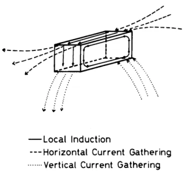
The low-frequency magnetic field induces regional electric fields (equilibrium fields) which are locally distorted by resistiv-ity heterogeneities.I recognize three different mechanisms re-sponsible for these perturbations at low frequencies: vertical current distortion, horizontal current distortion, and local in-duction. Figure 1 illustrates current patterns for these mecha-nisms. Current perturbations within any low-frequency band are caused by these three mechanisms acting simultaneously. The effects of one mechanism may dominate over the effects of others under certain geologic conditions. I deliberately chose models in which one mechanism, or a combination of two mechanisms, is the controlling factor for field distortions.

Current distortion mechanisms have essentially dc behavior-their electric field distortions are

frequency--

Local Induction

--- Horizontal Current Gathering

... Vertical Current Gathering

FIG. 1. Current patterns generated by distortion mechanisms around a conductive body.

independent at low frequencies. Local induction, however, pro-duces frequency-dependent effects. The regional magnetic field induces current cells in a good conductor. I use simple esti-mating methods to determine the order-of-magnitude effects of perturbations due to each mechanism and to examine three models whose fields exhibit current distortion and local induc-tion.

The electric fields presented in Table 1 are approximations of the contributions from each distortion mechanism. The esti-mate for each mechanism is made by solving analytically an appropriate simplified model.I use an analytic solution due to Ranganayaki and Madden (1980) for an anisotropic 2-0 thin layer to approximate the contribution from vertical current distortion. The contribution from horizontal current distortion is estimated using a simplified form of a solution due to Lee (1977) for a conducting ellipsoid. The electric field due to local induction is approximated using a wire loop with cross-sectional area equal to that of the heterogeneity. The details of these approximations are presented in the Appendix. Back-ground fields are also provided at each site. The backBack-ground field outside a heterogeneous feature is simply the 1-0 field. The background field inside a heterogeneous body is the average current density for the crust divided by the conduc-tivity of the body, in the absence of distortion mechanisms. This average current density is approximated from the outside 1-0 electric field. Note that my background field includes the "S effect" (Berdichevskiy and Dmitriev, 1976).

Vertical current distortion

Vertical current distortion is a result of resistive coupling between the upper crust and upper mantle. Figure 2 presents the modelIuse to illustrate the effects of vertical and horizontal current distortion. The model consists of an L-shaped valley with a resistivity of 10Q.m. The surrounding region has a resistivity of 400Q .m. The heterogeneous layer at the surface is underlain by the 1-0 structure also shown in Figure 2.Ireduce the resistivity of the 10 000Q .m lower crust to 1 000Q.m to illustrate the adjustment-distance effect. The adjustment dis-tance is a measure of how easily vertical current can flow into or out of a surface heterogeneity and is discussed in the Appen-dix. This distance is essentially a horizontal "skin depth" as-sociated with vertical current flow. The adjustment distance decreases as the resistivity of the lower crust decreases and vertical current flow becomes easier.

Table 1. Estimates of electric field contributions (inVim) from vertical current distortion (VCD), horizontal current distortion (HCD), and local

induction (LI) for models presented in Figures 2 and 5. Background fields are provided for reference. Background field outside a heterogeneity is the corresponding I-D field at infinity. Background field inside is the outside I-D current density divided by the conductivity of the heterogeneity. Contributions have been calculated for .01 Hz. Two sets of sounding curves are presented in each of Figures 3 and 4, so these sites are appended with the lower crustal resistivity used to generate the curves.

North-south contribution estimates East-west contribution estimates

Site VCO HCO LI Back VCO HCO LI Back

Figure 3(104) 10-3 2.6X 10-4 2.0X 10-5 10-4 4.1X 10-4 3.1X 10-5 2.0X 10-5 10-4 Figure 3 (103 ) 1.9X 10-3 _2.5X 10-4 2.2X 10-5 _9.0X 10-5 10-3 3.0X 10-5 2.0X 10-5 9.0X 10-5 Figure 4(104 ) 4.7X 10-4 2.5X 10-4 ₀ 3.9X 10-3 Not computed Figure 4(103 ) 10-8 2.4X 10-4 ₀ 3.7X 10-3 Not computed Figure 6 2.3 x 10-5 _{4.4X 10-}5 _{7.5X 10-}5 _{1.5X 10-}5 _{8.2X 10-}6 _{5.0X 10-}6 _{8.0X 10-}5 _{1.5X 10-}5

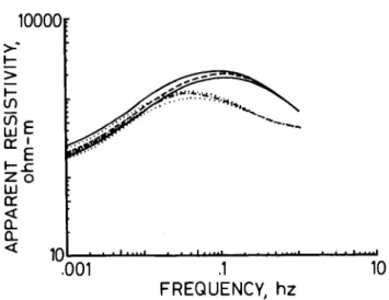
The sounding curves in Figure 3 are for site A within the conductive feature (Figure 2).Two sets of curves are presented: one for a lower crustal resistivity of 10 000Q.m (solid lines); and one for a lower crustal resistivity of 1 000Q.m (dotted lines). As Table 1 indicates, vertical current distortion is the dominant mechanism controlling field behavior inside the heterogeneity for both values of lower crustal resistivity. The electric field estimates given in Table 1 for Figure 3 are largest for vertical current distortion. The adjustment distance de-creases from 191 km to 136 km (see the Appendix) on reducing the lower crustal resistivity by an order of magnitude. Vertical current flow into the conductive feature thus becomes easier, and the sounding curves are shifted up for the model with the smaller lower crustal resistivity. The parallel offset in Figure 3 reflects the frequency-independent nature of vertical current distortion at low frequencies.

Theshapesof the curves (and hence the phases) to the left of the maxima in Figure 3 are dictated by the structure beneath the heterogeneous layer. The structure used here is

homoge-10000

E

I

E

s:

o

>~

t:

>

I-If) If) W 0:: I-Z W 0::

~

a..

<t

1.001

.1

FREQUENCY, hz

10

FIG. 3. Sounding curves generated at site A for structure in Figure 2 for lower crustal resistivities of 10 000 Q.m (solid curves) and 1 000Q.m (dotted curves). The correspondingI-D

curves outside the valley are shown for reference (dashed curve is for a lower crustal resistivity of 10 000Q .illand the dash-dot pattern is for a resistivity of 1 000Q.m). These curves were computed assuming the structure directly beneath site B ex-tends laterally to infinity. Maximum apparent resistivities are in the northwest-southeast direction, and minimum apparent resistivities are in the northeast-southwest direction.

MAP VIEW

B

::~'<>: ,,' ;

..

::.:'

r>,;;,

J:G'~j::j

rr=E

S

10000

FIG. 2. Model of L-shaped 10Q.m valley used to generate sounding curves in Figures 3 (site A) and 4 (site B). The map view shows the distribution of resistivity in the heterogeneous top layer, and the cross-section shows the layered structure beneath the heterogeneity. The resistivity of the 10 000Q.m layer is reduced to 1 000Q.m to produce the second set of sounding curves in Figures 3 and 4.

FIG. 4. Sounding curves at site B generated for the structure in Figure 2 for lower crustal resistivities of 10 000Q .m (dashed curves) and 1 000 Q.m (dotted curves). Maximum apparent resistivities are in the north-south direction, and minimum apparent resistivities are in the east-west direction. The corre-sponding I-Dcurves at this site are also shown (dashed lines). Note that two I-D curves are shown-one for each value of lower crustal resistivity (dashed pattern is for 10 000Q.m and dot-dash pattern is for 1 000Q .m).

10

.1

FREQUENCY, hz

10~"""""'...L..&.o.o.oL.-"""''''''''''''''''''''''''''''''''''''''''''''-'-'''''''''''''''

.001

>~

I->

I-If)

tDE

0:: 1

E

1-£

ZO

W 0::

<t

a..

a..

<t

3030 ohm -m

50 km

100 ohm-m

50 km

50 ohm-m

150 km

10 ohm-m

Shaded =10 ohm-m

CROSS-SECTION

-4--0-0-o-h-m--m-~-:;:'Z"'>ti:,:"

!J<m

4km

50 kmI

neous, so the low-frequency portions of the sounding curves resemble the outside I-D curve (dashed line). The extrema on the sounding curves in Figure 3 between .01 and .1Hz are not due to deep structure, but are caused by surface heterogeneity. The resistivity contrast, thickness, and size of the heterogeneity control the amount of shift and location of inflection points. The result is a curve which resembles a shifted version of the outside I-D curve at low frequencies.

distortion is dominant. Minor changes will result if horizontal current distortion is dominant. Minor shifts in the sounding curves are observed as the adjustment distance is decreased by a factor of 3. The ratio of the maximum to minimum apparent resistivity curves remains the same. Horizontal current distor-tion is thus the dominant mechanism. This type of distordistor-tion also results in parallel offset sounding curves because it is a frequency-independent effect at these low frequencies.

Horizontal current distortion

Local induction The effect of a heterogeneity upon the fields at a distant site

diminishes as the adjustment distance decreases. The sounding curves at site B in Figure 2 are shown in Figure 4. This site is in a locally I-D environment, yet the sounding curves indicate heterogeneity. Site B is 5 adjustment distances from the L-shaped valley for the lower crustal resistivity of 10 000

n·

m and 18 adjustment distances for the resistivity of I 000

n·

m. Accordingly, vertical current distortion is expected to be rela-tively more important at site B for the more resistive lower crust. Comparison of the electric field estimates for Figure 4 given in Table I shows that horizontal current distortion is the dominant mechanism for the lower crustal resistivity of I 000

n .

m. Independent confirmation of the dominance of horizon-tal current distortion is shown in Figure 4. Reduction of the lower crustal resistivity should produce significant differences between the two sets of curves in Figure 4 if vertical current

The distortion mechanisms discussed thus far produce frequency-independent shifts of sounding curves at low fre-quencies. The sounding curves within a heterogeneity resemble shifted versions of the I-D sounding curve outside the hetero-geneity. Local induction, however, is a frequency-dependent phenomenon. Apparent resistivity as expected to be pro-portional to frequency[E'J.ffrom equation (A-13) and Pa'J.Ez/

fJ

in the absence of other mechanisms. This frequency-dependent offset from the outside I-D curve is seen in the sounding curves at site A which is shown in Figure 5. These sounding curves are presented in Figure 6.

The shape of the north-south apparent resistivity in Figure 6 is more similar to that of the outside I-D curve than is the shape of the east-west apparent resistivity. I deduce from the electric field estimates for Figure 6 in Table I that current

10

.1

FREQUENCY, hz

100

E

I

E

J:.

o

>'

~

>

~ t/) t/) W 0:: ~ Z W 0::

~

c,

<{

.o~OO1

4

km

24

km

MAP VIEW

""A';

..

:;':)'

....

,

':':

Shaded: 1 ohm-m

CROSS SECTION

-10-0-0-h-m---m--""~---1000ohm-m

rF

E

S

50kmI

20 ohm-m

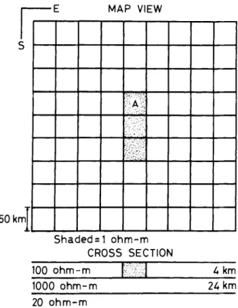
FIG. 5. Model of In·m conductor used to generate sounding curves in Figure 6 (site A). The conductor consists of a 50 km wide, 150 km long, and 4 km thick body. Model presentation is identical to that in Figure 2.

FIG. 6. Sounding curves inside a good conductor (site A in Figure 5). The corresponding I-D curve (dashed line) outside the conductor is shown for reference. Maximum and minimum apparent resistivities are labeled with their appropriate direc-tions. Fields were only computed up to frequencies of.1 Hz because of numerical inaccuracies at higher frequencies for this conductor.

distortion and local induction are equally important in the north-south direction. Local induction effects are an order of magnitude larger than those of current distortion in the east-west direction, however. Evidence for this conclusion consists of the steeper slope on the east-west sounding curve in Figure 6 and the electric field estimates for Figure 6 in Table 1. The balance between current distortion and local induction is af-fected by two factors in this case. First, induction in thin, tabular bodies [see equation (A-13)] is independent of geome-try except for thickness. The contribution from local induction is thus almost constant for the north-south and east-west direc-tions (some variation exists because of magnetic field differ-ences for these directions). Second, current distortion effects in a particular direction inside a heterogeneity are increased by lengthening the body in that direction. More vertical current may be attracted by a longer conductor (see the Appendix). Current distortion is hence relatively more important in the north-south direction than in the east-west direction.

Local induction effects enhance the electric field within a conductor. This is enhancement over the background field, however, not the inside 1-0 field. The background field (1.5

x 10-5

Vim) is much smaller than the inside 1-0 field (2.9 x 10 -4 V/rn)for the model in Figure 5, and adding an

induc-tion term (7.5 x 10-5V/m) does not raise the total field to the

level of the I-D field. It is thus possible to produce apparent resistivities that are less than intrinsic resistivities and still have local induction as the dominant mechanism.

Summary

Heterogeneities distort the low-freq uency "eq uilibrium " fields in different ways, depending upon which mechanism is dominant. The perturbations appear as parallel offsets of sounding curves when current distortion is important. The principal difference between horizontal and vertical current distortions is that the variations decay away from the contacts differently [see equations (A-3), (A-4), and (A-IO) in the Appen-dix]. Local induction effects, however, are frequency-dependent distortions. These effects are only seen in regions where interac-tion of the source field with high resistivity contrasts (100: I or larger) produces closed current cells.

BEOWAWE KGRA, NEVADA

I now present MT sounding curves from the Beowawe KGRA in Nevada which exhibit both the current distortion and local induction effects discussed above. I discuss the inter-pretation of these data, highlighting evidence for these mecha-nisms. These data were collected by Geotronics Corporation for Chevron Resources Company, and they were qualitatively interpreted by Swift (1979), My interpretation substantially agrees with Swift's, with one exception as noted.

Removal of surface heterogeneity

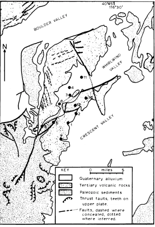
The locations of the 11 sites used from this survey are shown on a generalized geologic map in Figure 7. I have grouped these sites according to geographical location and similarity in sounding curve shape and overlain the curves in Figures 8 and 9. The curves roughly cluster into one set to the northeast and another to the southwest.

The effects of surface heterogeneity are next removed from these sites. I conclude that the dominant mechanism is current distortion (both horizontal and vertical) from the parallel off-sets of the sounding curves in the frequency range 10-100 Hz. The surface heterogeneities are so thin that their effects are frequency-independent below 100 Hz. Simple shifting of the sounding curves is thus justified. The sounding curves are aligned with a representative "average" curve at high fre-quencies(f > 10 Hz). This shifting to a representative curve at high frequencies preserves the information about deeper struc-ture present at the lower frequencies (f < 1 Hz). The corrected curves are presented in Figures 10 and 11, which I call "gener-alized sites 1 and 2," respectively.

Effect of surrounding basins

I constructed a model accurately reflecting the 3-D hetero-geneity of the top 1 500 m at Beowawe to examine the effects of the alternating basin-outcrop structure. This model was based upon drill holes, gravity data (Erwin, 1974), surface geology (Figure 7), and de resistivity (Smith, 1979). Smith (1979) ob-served that resistivities of the alluvium in Whirlwind Valley differed little from those of the surrounding outcrop. Whirlwind Valley is only 50 m deep, based on drilling information (Chevron Resources Company, 1976). Hence, all the sites essen-tially lie above resistive (-100

n·

m) material. Small splits in the sounding curves, with maximum-to-minimum apparent re-sistivities at 100 s periods of 1.5, result from distortion of the fields by the neighboring valleys. A structure consisting solely of the observed laterally heterogeneous features is an inad-equate model for Beowawe, and deeper structures must be present.

Two-dimensional interpretation

The direction of maximum apparent resistivity is consistently northeast-southwest at low frequencies, based upon the rota-tion angles for these sites. The tipper direcrota-tions, however, show a consistent northwest-southeast trend for regional current flow. (The 3-D model discussed above was incapable of produc-ing these rotation angles and tipper directions.) Stewart et al. (1975) inferred a series of north-northwest trending diabase dikes beneath this region based on aeromagnetic data and geologic evidence. Proprietary MT data (Chevron Resources Co., 1976) to the southeast closely resemble our sounding curves and rotation angles. I conclude from all of these data that my sites lie over an elongated, anisotropic body with a northwest strike direction. I was unable to produce an isotropic body over which the direction of maximum apparent resistivity was at right angles to the direction of current flow. [Swift (1979) also concluded that Beowawe must be underlain by an aniso-tropic body.] The anisotropy is not an intrinsic material property- it results from fine-scale heterogeneity. Vertically emplaced resistive dikes intruding into conductive sediments would produce a structure which is resistive across strike and conductive along strike. The direction of maximum apparent resistivity is just the direction of maximum electric field, and the present anisotropic feature as described would produce this same maximum direction.

Evidence of current entrapment in the upper crust can be seen in Figure 1I. The maximum apparent resistivity is

790

versely proportional to frequency in the range .01-.1 Hz. The impedance

I

E/H

Iis thus constant in this frequency band.

Cur-rent is not escaping into the mantle at the lower frequencies, or the impedance would decrease.I infer from this that the lower crust must be resistive in order to trap this current. My con-clusion here differs from the concon-clusion reached by Swift (1979) that the lower crust must be conductive. My structure is a buried, elongated feature with a northwest strike direction. The body is conductive along strike and resistive across it. This body is underlain by a resistive lower crust. The cross-section of

a 2-D model which yields a good fit to the sounding curves in Figures in Figures 10 and 11 is shown in Figure 12.Iuse a 2-D model because it satisfactorily fits all of my data and the ge-ology. Three-dimensional modeling is not justified in this case, except to verify that the 2-D model is adequate.

Current distortion effects are seen when comparing the maxi-mum apparent resistivity curves in Figures 10 and 11. The low-frequency portions of these curves are parallel, but offset. Current distortion is the dominant mechanism in the northeast direction. The maximum curve in Figure 11 is lower than that

Quaternary alluvium Tertiary volcanic rocks Paleozoic sediments Thrust faults, teeth on

40°45' 116°30' 5 I miles

o

I

N

FIG. 7. Generalized geologic map of Beowawe, Nevada (after Roberts et aI., 1967, and Stewart et aI., 1977). MT sites are heavy black dots, and site numbers are shown.

W l./l

«

I

0-90

1~

1 3 4

o

1000

>"

₁₀₀

~

s

~ (/)

iii

wE

10

cr:1

~E

z.c

WO

a:

~

0-«

.1.

₀₀₁

_.01

_.1

₁

₁₀

₁₀₀

FREQUENCY, hz

.01

.1

1

10

FREQUENCY, hz 3 1

.1L....-"--'-...

- - ' - - - - ' - - - o . . -...- ' - - - ' - - '

.001

100

-901..----"--'---'-"""---'---'----'---""--'

1000

>'

~

>

100

tn

~E

cr: I 10

~E

z.c

WO

cr:

~

0-«

FIG. 8. Sounding curves for generalized site 1 uncorrected for surface heterogeneity. Individual phase plots for sites 10, 11, and 12 are not shown because of congestion on plot.

FIG. 10. Sounding curves at generalized site 1 corrected for surface heterogeneity. A good fit (dashed line) to the data generated with the model in Figure 12is shown.

W l./l

«

I

0-90

~

o

100

.01

.1

1

10

FREQUENCY, hz

1000

>"

5;

100

~ l./l if)

wE

10

cr:.

~E

z.c

WO

cr:

«

0-«

Dl

.1

1

10

FREQUENCY, hz .1 '--_..._--1.--1._--'--'-_-'-..._ ...

.001

100

7

-90

L....---'-..._ " - - ' - _ - - - ' - - ' - - - "..._~

1000

>' ~

>

100

~ (/)

~E

cr: I 10

~E

z.c

WO

cr:

~

0-«

FIG. 9. Sounding curves for generalized site 2. These are not yet corrected for surface heterogeneity. Individual site numbers are shown next to each curve.

FIG. 11. Sounding curves at generalized site 2 corrected for surface heterogeneity. A good fit (dashed line) to the data generated for the model in Figure 12is shown.

792

(1) in Figure 10, so generalized site 2 is closer to an edge of the buried feature. The lack of shape similarity for the maximum and minimum curves in either Figures 10 or 11 suggests that local induction is important in the northwesterly direction. The minimum apparent resistivities decrease proportionally with frequency, which also suggests local induction effects. Local induction occurs only when the structure is very conductive, so the feature is conductive in the northwest-southeast direction. The structural inferences drawn from analysis of the distortion mechanism evident in the data thus confirm certain aspects of my qualitative interpretation.

I deduce from my analysis of local induction that the length (or width) of a thin, tabular body is not a critical feature of the model. Equation (A-13) reduces to

jrollH~Z Ein •1= 2 '

if ~y ~ ~Z. Induction effects are dependent only upon the thickness of the conductive feature. The sounding curves for the generalized sites were fitted with sounding curves generated using a 2-D modeling program, although the structure is 3-D. The 2-D sounding curves in Figures 10 and 11 do not change appreciably when the 2-D body is truncated because local induction dominates the field behavior in the northwest direc-tion.

The effects of truncation upon the sounding curves from the 2-D model have been examined, and the results from this test are shown in Table 2. The apparent resistivities presented in Table 2 were generated for a frequency of .01 Hz using my 3-D modeling program. I varied the length-to-width ratio (aspect ratio) for a conductive valley. The cross-section of the conduc-tive valley was identical to that in Figure 12, except that the

anisotropic body was replaced by an isotropic, 1

n .

m conduc-tor. The apparent resistivity along strike only varied by 30 percent as I changed the length-to-width aspect ratio from00 to 1. (Any observation concerning the apparent resistivity across strike is irrelevant because the model is also conductive in that direction.)

Summary

I used the insights learned from my study of distortion mech-anisms to interpret MT data from Beowawe qualitatively. Comparison of sounding curves from different sites yields evi-dence of current distortion. This evievi-dence is used to constrain the structural geometry. The steep slopes for the minimum apparent resistivities indicate local induction effects, and thus the structure is conductive in the northwest-southeast direc-tion. I am not able to limit the length along strike of our buried feature. I can only establish a minimum length of 120 km from the present study of aspect ratios (Table 2).

FORMULAnON

The synthetic sounding curves examined above were gener-ated using a 3-D modeling program discussed in Madden and Park (1982). The program is based on an extension of the generalized thin sheet analysis (Ranganayaki and Madden, 1980). Their original work used only one heterogeneous layer, while I can stack many heterogeneous layers to build up a general 3-D medium. The following is a brief review of the theory behind the modeling algorithm.

Conductivities in the crust range from .00001 U/m to10U/m, so displacement currents are much smaller than conduction currents for the MT method. Maxwell's equations thus reduce to

"Denotes test of repetition assumption using rectangular blocks with aspect ratio of 3 :1.

Table 2. Apparent resistivity changes caused by varying length along the strike of a good conductor. All apparent resistivities are in

n .

m. These calculations were made for an isotropic 1

n .

m conductor 6.6 km thick using my 3-D modeling program.

Aspect Paacross p,along

ratio Model size strike strike

00 40 km x 00 .58 1.56

7: 1 40 km x 280 km .58 1.93

3: 1 40 km x 120 km .56 1.74

3: 1

*

40 km x 120 km .60 1.52

1 : 1 40kmx40km .99 .99

using a time dependence of exp (-jrot). Assume that the medium is transversely isotropic, with the z-axis as a symmetry axis. The conductivity tensor may thus be partitioned into a horizontal conductivity tensor [qs]and a vertical conductivity

qe ' This generalization allows modeling of the anisotropic

conductivity, if desired. The conductivity tensor for the medium is thus (2) (3)

v

xE=jrollH

v

x H= crE and

SSW

G.

y.l

Gf"2

NNE

200 ohm-m .2 km 10 ohm-m .2 km .2km

T

10/200'"

10123

2.2 km 1.2 ki '--,

S120()

" 100 ohm-m

t

.3/23

3.2 krr

.3/20'0

, 1-14.4 km--j7.2 km 1000 ohm-m 24 km 20 ohm-m

FIG. 12. Cross-section for 2-D anisotropic structure used to generate curves of good fit in Figures 12 and 13.The locations of generalized site 1 and 2 are shown. The anisotropic section is indicated by the stippled area. The first number within the anisotropic section is the resistivity parallel to strike, and the second is the resistivity across strike. The strike of the model is north-northwest/south-southeast.

I rewrite Maxwell's equations in terms of the horizontal electric and magnetic fields (E" H.) and the vertical fields (Ez' Hz), and substitute the expressions for the vertical fields into those for the horizontal fields.Maxwell's equations thus become

oH,/oz

= _-iz

x

(q,E,)

+

_Vs[(VsxEs)' iz/(jO)~)], (6)

where E.

=

(Ex, Ey) , H,

=

(Hx' Hy) , V,

=

(a/ax, %y), pz

=

l/oz ' and i, is the unit vector in the z-direction (downward). This formulation is similar to that of Ranganayaki and Madden (1980).

The vertical derivatives in equations (5) and (6) are approxi-mated using finite differencing (hence the term "thin sheet") and get

layersH'Bis completely represented by a finite-length Fourier series with exponential terms exp (jk~x

+

jk~y). A fast and efficient procedure for computing the set of all possible solu-tions is to propagate the fields formed with each exponential term up through the heterogeneous stack separately. The fields so propagated will not be composed of a single exponential term at the surface, but they will contain the complete set of exponential terms. The heterogeneous conductivity structure imparts a wavenumber structure to the fields at the surface. I use(k~, k~)to denote the original wavenumber structure chosen for the starting fields and(kx 'ky )to denote the total

wavenum-ber structure.

The Fourier coefficientA(k~, k~)for each exponential is ini-tially unknown, but is determined by solving a set of simulta-neous equations representing the source and boundary con-ditions at the Earth's surface. I must use two orthogonal polar-izations becauseHsBis a vector. The two trial forms forH'Bare thus

q=[[O.]

[O]J.

[0] a;

oE./oz

= -jO)~(iz xH)

+

Vs(pz(VsxH,)' iz), and

E,+= E.-

+

ilz{jO)~(iz

x

H.-)

- V,[Pz(V,

x

H,_)'iz] } (4) (5) (7) and HsB= (A,0) . exp (-. '), H'B= (0,A') •exp (.. -). (9) (10)

whereE.+and Hs+ are the fields above the thin layer, and Es

-and Hs - are the fields below the thin layer. Equations(7)and (8)

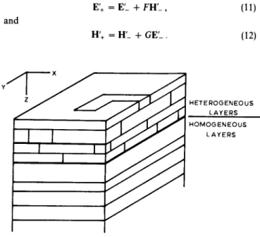
are used to continue fields across a heterogeneous thin layer. The heterogeneous thin layers are stacked to build up a general 3-D medium (Figure 13) and continuity of tangential fields is used to continue the fields from one thin layer to the next.

The horizontal derivatives in equations (7) and (8) are not approximated using finite-differences because I use a horizontal step size equal to the smallest scale length for conductivity variations. Instead I assume the conductivity structure, and thus the field variations, are accurately represented with a finite set of wavenumbers. Horizontal derivatives are computed ex-actly in the wavenumber domain using wavenumber multipli-cation. This assumption places restrictions upon the model: the structure shown in Figure 13 repeats indefinitely in the x- and j-directions, and the minimum wavelength of the lateral he-terogeneities must be greater than the Nyquist wavelength.

The results of a test of the effects of model repetition are included in Table 2. The second entry for an aspect ratio of 3 was calculated using a single, rectangular block 40 km by 120 km. This change moved the nearest north-south image feature 4 times farther away. The apparent resistivity along strike is' virtually unchanged from the 2-D value. I thus believe most of the variability seen in Table 2 is due to repetition effects and not truncation of the 2-D body.

Spectral analysis (Orszag, 1972) is used for the fields at the Earth's surface. I first find all possible solutions to the problem (a finite set because I am restricted to a finite set of wavenum-bers) and then apply source and boundary conditions at the Earth's surface. These boundary conditions allow me to com-bine my set of all possible solutions into a single solution which simultaneously satisfies Maxwell's equations and the boundary conditions everywhere.

The next step is to determine the set of all possible solutions. The magnetic field at the bottom of the stack of heterogeneous

FIG.13.Stack of heterogeneous and homogeneous layers used by modeling algorithm. Coordinate system is shown (not to scale).

An impedance boundary condition is applied at the bottom of the heterogeneous stack to account for the medium beneath the stack. The electric field corresponding to H'Bis thus E.B(k~, k~)= ~(k~, k~), H'B(k~, k~).The magnetic fields given by equa-tions (9) and (10), and their corresponding electric fields, are continued up through the heterogeneous stack to the Earth's surface using equations (7)and (8). The continuation is done for each possible(k~, k~)wavenumber pair.

The Fourier coefficientsAandA'are carried up through the stack oflayers without modification because the Fourier trans-form, the tensor impedance~(k~, k~),and the differential oper-ators in equations (7) and (8) are linear operoper-ators. Suppose one wants to continue (E'+, H'+)= (AE_ , AE_) up through one layer. Equations (7) and (8) can be represented by the linear equations (11) (12) HETEROGENEOUS LAYERS HOMOGENEOUS LAYERS E'+= E'_

+

FH'_ , H'+= H'_

+

GE'_ . and (8) H,+ = H.-

+

_ilz{iz

x

(q.E._) - Vs[(Vs

x

E._) .iz/(jO)~]}, and

Substitute (E'_ ,H'_) into equations (11)and (12)to get E'+ = AE_

+

AFH_

and

(13)

(14)

been used, under the assumption of a finite set as a starting solution. The fields at the Earth's surface are thus given by

Esr(k x' ky)=

I I

A(k~, k~)

(17) I use the linearity properties ofF and Gand the definitions

E+= E_

+

FH_ and H+ = H_

+

GE_to rewrite equations (13)and (14) and Hsr(kx ,ky)=

I

L

A(k~, k~) "x' k y' (15) (18) and

The coefficient multiplying(E+, H+)is the samescalar con-stant multiplying (E_, H_). There is a unique, but undeter-mined, coefficientA(k~, k~)_{for each trial value of HsB.}

Our set of all possible solutions at the Earth's surface is complete because

H

sB is completely characterized by a finite Fourier series. Every possible horizontal wavenumber pair has

(20) (19)

Comparison to 2-D modeling

Equation (20) gives one equation for each unique (kx 'ky )pair,

so one can solve for A(k~, k~). Substituting these coefficients back into equations (17)and (18) yields the surface electric and magnetic fields.

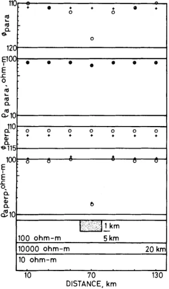
The above assumption that the conductivity structure is accurately represented with a finite set of horizontal wavenum-bers forces the structure to repeat indefinitely. Image structures may contribute to field changes near the primary structure being modeled. Figure 14 presents a comparison ofresults over a 2-D body computed using the algorithm described above and a 2-D network modeling program (Madden, 1971). The body has infinite length along strike for both programs, but the 3-D program has image conductors spaced every 180 km apart. My model with its imaged conductors has an effective horizontal conductance for the top layer 11 percent higher than that for the network model with its single conductor. More current flows in the heterogeneous layer of my model than that for the network model, but the outside resistivity is the same. Hence, the perpendicular apparent resistivity (Po) outside the hetero-geneity is larger for the 3-D program than for the network program. This difference is apparent in Figure 14. The in-creased horizontal conductance also affects the phase of the perpendicular magnetic field. Thus, the phase of the parallel Po differs (Figure 14). Results from the two modeling programs otherwise agree. I then expect field errors of a few percent due to the repetition assumption in the following analysis of distor-tion mechanisms.

where Es(kx , ky:k~, k~) and Hs(kx , ky:k~, k~) are the fields

computed for each one of the starting wavenumber pairs(k'x,

k'y).

I use a current sheet at the Earth's surface as a source and an outgoing admittance condition to represent the air (Ranganay-aki and Madden, 1980). The surface boundary condition is thus

L L

A(k~, k~)[Yair(kx, ky)Es(kx, ky,:k~, k~)

k:r.' ky'

Substituting equations (17) and (18) into equation (19) and rewriting to get a system of equations involvingA(k~, k~),there results (16)

130

70

DISTANCE, km

10

+

•

+ + + (I ₊ 0 0 0

•

•

•

_•

•

•

•

0 0 0 0 0 0 0 + + + + + + + +

"

0 0 0 u b tic':.;",':"';'!

1 km

100 ohm-m

5km

10000 ohm-m

20 km

10 ohm-m

120

E100

I E

.c

°

_to

...

to

a.

to

a...

10

d

10

...

(1)

a.

$115

100

E

I

E

.c

0.

a.

_...

(1)

a.

cfl0

to

...

to

a.

&

110

FIG. 14. Comparison of apparent resistivities and phases from Madden's 2-D network modeling program (0) and my 3-D modeling program (+). Resistivities and phases parallel to strike are shown on top, and those perpendicular to strike are below. The resistivity of the stippled zone is 10

n·

m.

CONCLUSIONS

I have presented a method for modeling magnetotelluric fields near 3-D structures. Analysis of modeling results shows

that fields near such structures are perturbed by three distor-tion mechanisms: resistive coupling of the upper crust and electrical mantle; resistive coupling between conductive fea-tures in the upper crust; and induction oflocal current loops in good conductors: My analysis was done for a conductive body in a resistive host, but the first two mechanisms still appear in the problem of a resistive feature in a conductive background.

All three mechanisms produce different spatial and frequency behavior in data, so identification of the dominant mechanism can aid an interpretation. I have shown an example of such an interpretation with data from the Beowawe KGRA in Nevada.

I am presently developing an efficient 3-D inversion based on our forward modeling scheme. Generalized reciprocity (Lanczos, 1956)is used to express the surface field change due to a conductivity perturbation in terms of the solution to the adjoint problem.Itis hoped this inversion will lend insight into thequestionof uniqueness for 3-D structures.

ACKNOWLEDGMENTS

This paper is a summary of a recently completed thesis, and it is not possible in this space to acknowledge everyone who has contributed to this work. lowe a special debt of gratitude to Ted Madden. Many of the ideas presented here originated with him, but in his usual humble style, he refused to be a coauthor because he felt he had not contributed enough to this work. I would also like to thank Alex Kaufman for directing me to the work by Berdichevskiy. The work presented here has been supported by the U.S. Geological Survey, the U.S. Department of Energy, Chevron Oil Field Research Company, and the Dept. of Earth, Atmospheric, and Planetary Sciences at the Massachussetts Institute of Technology.

REFERENCES

Berdichevskiy, M. N., Dmitriev, V.I.,Yakovlev,I.A.,Bubnov, V. P., Konnov, Yu, K., and Vartannov, D. A., 1973, Magnetotelluric sounding of a horizontally inhomogeneous media: Izv., Earth Phys-ics,1, 80-92.

Berdichevskiy, M. N., and V.I. Dmitriev, 1976, Basic principles of interpretation of magnetotelluric sounding curves,inAdam, A., Ed., Geoelectric and geothermal studies: Budapest, Akademai Kiado, 165-221.

Cagniard, L., 1953, Basic theory of the magnetotelluric method of prospecting: Geophysics 18,605~635.

Chevron Resources Company, 1976, Well summary report for Ginn no. 1-13 well.

Erwin,J. W., 1974, Bouguer gravity map of Nevada, Winnemucca sheet: Nevada Bur. of Mines and Geo!. Map 47.

Lanczos, C, 1956, Linear differentialoperators: D. Van Nostrand Co. Lee, T. C, 1977, Telluric anomalies caused by shallow structures:

Ellipsoidal approximations: Geophysics 42, 97-102.

Madden, T.R., 1971, EMCDC: Two-dimensional network modelling program.

- - 1980, Lower crustal effects on magnetotelluric interpretations or pulling the mantle up by its bootstraps: Workshop on research in magnetotellurics: implications of electrical interpretation for geo-thermal exploration, Napa Valley, February.

Madden, T. R., and Park, S. K., 1982, Magnetotellurics in a crustal environment: USGS Final Rep. 14-08-oo1-G-643.

Morrison, H. F., Lee, K. H., Oppliger, G., and Dey, A, 1979, Mag-netotelluric studies in Grass. Valley, Nevada: Lawrence Berkeley Lab. Rep. LBL-8646.

Orszag, S. A., 1972, Comparison of pseudospectral and spectral ap-proximation: Stud. App!.Math. 51, 253-259.

Park, S. K., Orange, A. S., and Madden, T. R., 1983, Effects of three-dimensional structure in magnetotelluric sounding curves: Geophys-ics,48, 1402-1405.

Ranganayaki, R. P., 1978, Generalized thin sheet approximation for magnetotelluric modeling: Ph.D. thesis, Massachusetts Inst. of Tech.

Ranganayaki,R. P., and Madden, T. R., 1980, Generalized thin sheet analysis in magnetoteliurics: an extension of Price's analysis: Geo-phys. J. Roy. Astr. Soc.,60, 445-457.

Roberts, R. 1., Montgomery, K. M., and Lehner, R. E., 1967,Geology and mineral resources of Eureka County, Nevada: Nevada Bur. of Mines and Geo!. Bull.64.

Smith, C, 1979, Interpretation of electrical resistivity and shallow seismic reflection profiles, Beowawe KGRA, Nevada: Univ. Utah Res,Inst. Rep. ESL-25.

Stewart, 1. H., Walker, G. W., and Kleinhampl, F. J., 1975, Oregon-Nevada lineament: Geology,3, 265-268.

Stewart, 1. H., McKee, E. H., and Stager, H. K., 1977, Geology and mineral deposits of Lander County, Nevada: Nevada Bur. of Mines and Geo!. Bul!., 88.

Strangway,D. W., Swift, C. M., Jr., and Holmer, R.

c.,

1973, The application of audiofrequency magnetotellurics to mineral explora-tion: Geophysics,38, 1159-1175

Stratton, J. A., 1941,Electromagnetic theory: McGraw-Hili Book Co. Swift, C. M., Jr., 1967,A magnetotelluric investigation of an electrical

conductivity anomaly in the southwestern United States: Ph.D. thesis, Massachusetts Institute of Technology.

- - 1979, Geophysical data, Beowawe geothermal area, Nevada: Trans., Geothermal ResourcesCouncil 3, 701-703.

Vozoff, K., 1972, The magnetotelluric method in the exploration of sedimentary basins: Geophysics,37,98-141.

APPENDIX

I present in this appendix the simple methods I used to estimate the order-of-magnitude contributions from each of the distortion mechanisms discussed. The estimation procedures used for vertical and horizontal current distortion are de ap-proximations. The estimates are thus only valid at low fre-quencies where the thickness of the heterogeneous region is much greater than the skin depth. All estimates are based upon a rudimentary knowledge of the geometry and conductivity of the structure, so they may also be used as an interpretational aid.

Vertical current distortion

Consider vertical current distortion first. Ranganayaki and Madden (1980) gave the solution for the perpendicular electric field over an anisotropic thin sheet (see Figure A-I):

O"IEOI- 0"2 E02 E 1= Eo 1 - --=.---"--'---=-..::.:.

0"1+0"2

Xexp [ -

I

xI/j(0"ILiZ1P1LiZ2)], (A-I) and

O"IEOI - 0"2 E02

E2= E02

+

r==========='=

j(O"I + 0"2) + 0"2

Xexp [-lxIIJ(0"2 LiZ1P2LiZ2)], (A-2) whereEo Iand_E02are the respective1-0solutions,0" Iand0"2

are horizontal conductivities, and PI and P2are vertical re-sistivities. Observe from equation (A-2) that the electric field is enhanced on the resistive side of the contact (side 2) because the conductor attracts current. This excess current is responsible for the electric field distortion. Thedistortionis thus given by

0" IE o1 - 0"2 E02

LiEoutVCG= --='r======~

, J(0"10"2)+ 0"2

X exp [-lxl/j(0"2LiZ1P2LiZ2)]. (A-3) The field on the conductive side of the contact (side 1) is depressed and reaches a minimum at the contact. The field increases as we recede from the contact because vertical current flows into the conductor. The field increase caused by vertical

current flow is the difference between the field in equation (A-I) and the field at the contact, and is

x[I - exp [-lxl/J(0"18IPI8Z2)]. (A-4) The parameter given by J(0"18ZIPI8Z2) is called the "ad-justment distance" (Ranganayaki and Madden, 1980) and is a measure of how easily vertical current is attracted by a conduc-tor. The adjustment distance is calculated from the integrated conductance (0"8Z

d

of the surface layer and the integrated resistance (p8Z2) of the underlying structure. A resistive lower crust prevents current flow from the mantle, and fields would

thus remain depressed inside a conductive feature for many kilometers. Both field distortions in equations (A-3) and (A-4) have exponential behavior, so the adjustment distance is essen-tially a horizontal "skin depth" associated with vertical current flow. Finally, the distortions in equations (A-3) and (A-4) are frequency-independent in the frequency ranges where thin-sheet analysis (Ranganayaki and Madden,1980)is valid.

Horizontal current distortion

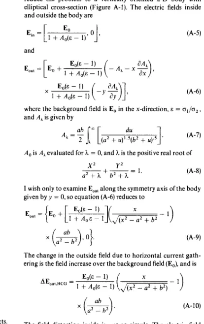
Isimplify the solution by Lee(1977)for telluric fields around a 3-D ellipsoid to estimate horizontal current distortion effects. His solution for the 3-D ellipsoid contains both horizontal and vertical current effects, but I want just horizontal ones. I thus reduce the problem to a vertically oriented 2-D body with elliptical cross-section (Figure A-I). The electric fields inside and outside the body are

[ Eo

J

E· = 0 In I+A_o{e-l)' , and (A-5) (A-6) (A-7)

x

EOU I= [Eo

+

I

:o~eo~ ~

I) ( - A, - x

aa~)

x Eo(e - I) (_

YCA,)]

I

+

Ao(e - I) iJy'

where the background field isEo in the x-direction,e= 0" I/O"2' and A, is given by

A,=

a;

fO

[(a

2

+

U/5~b2

+

U).5}

A_oisA, evaluated forA. = 0,and A.is the positive real root of

(A-8) Iwish only to examineEOU Ialong the symmetry axis of the body

given byy= 0, so equation (A-6) reduces to

(A-9)

0",

sz,

The change in the outside field due to horizontal current gath-ering is the field increase over the background field(Eo),and is

FIG. A-I. Models used to estimate current distortion effects. The upper model is used for horizontal current distortion (HCO), and the lower model is used for vertical current distor-tion (VCO). The upper model is a vertical body of ellipsoidal cross-section as shown and conductivity 0"1 immersed in a

homogeneous medium with conductivity 0"2' The background field is shown byEo. The lower model is that of an anisotropic thin sheet. The sheet is divided into two half-planes, each with vertical resistivity Pi' horizontal conductivity 0"; and total thickness 8Z 1

+

8Z2 •

The field distortion inside is not so simple. The electric field change due to excess current attracted to the conductor is needed. The background current density is 0"2Eo in the absence of the elliptical body. Idefine the" background" field inside as that field which would be present if the background current density were flowing in a uniform conductor with conductivity

('JI' This is identical to the treatment by Berdichevskiy and

Dmitriev (1976) of their" S effect". The background field inside

is thus Eo/c, and the distortion inside caused by horizontal

current gathering is

1

E·dt= jWIl

1

H·da, (A-I3)

Local Induction

The electric field perturbations due to horizontal current dis-tortion vary as a low-order polynomial in distance outside the heterogeneity and are constant with position inside. These solu-tions are strictly de solutions, so they only apply at low fre-quencies. (A-IS) (A-I4) k2 ₁ Ell>= - .

I

m

I

sin

e,

4n

J~ (~

kR 2 ) c R

+

kR2

whereE. is the cj>component in a spherical coodinate system aligned along the axis of the horizontal dipole, R is the distance to the dipole, andk2

= w21lc.

The simple-minded estimates in equations (A-3), (A-4), (A-IO), (A-II), (A-14), and (A-15) for field perturbations due to vertical current distortion, horizontal current distortion, and local induction are approximate at best. None of the models used to derive these estimates are accurate representations of 3-D bodies. The estimates thus only suffice for an order-of-magnitude study of the dominant distortion mechanism. Equation (A-14) also gives the distortion caused by local induc-tion because this mechanism contributes nothing to the back-ground field. Local induction effects will also exist outside the conductive body. An approximation of these effects is the field due to a horizontal magnetic dipole with moment

m

= I(A Y6Z).Stratton (1941) gave the far-field electric field for this dipole as

where

A

is the area encircied by the path

t.

The area of the current loop is roughly the cross-section of the body (AYlong and AZ thick), and Eis assumed constant on the path. Evalu-ation of equEvalu-ation (A-I3)yields

(A-II)

(A-12)

Eo Eo

6E. HCG= "

-In. 1

+

Ao(c

+

1) c

The last mechanism I examine is local induction. The ac magnetic field induces current cells in a conductive body. The magnetic field has a large, spatially constant component (80--90 percent of the total field) within the body, and this component is coupled to internal current cells. An analysis of the transient response of a dissipative waveguide shows that the fundamental mode of excitation decays least fast. I assume that only the fundamental mode is present for this approximation. The decay time for

a

2-D conductor of width!l.Y and thickness !l.Zin an insulating medium is

The lowest order mode is given bym= n= 1, and the decay time for this mode for the conductor in Figure 5 is 13 s. Hence, the decay time is in the range of periods in which we are interested. The electric field due to this coupling is estimated using Faraday's law