EDDY HEAT FLUXES AND STABILITY OF PLANETARY WAVES by
CHARLES AUGUSTIN LIN
B.S., University of British Columbia (1974)
SUBMITTED IN PARTIAL FULFILLMENT OF THE REQUIREMENTS FOR THE
DEGREE OF
DOCTOR OF PHILOSOPHY
at the
MASSACHUSETTS INSTITUTE OF TECHNOLOGY May, 1979
Signature of Author . . . . . . . . . . . . . . . . . . . . . . . . . . . Department of Meteorology, May 1979 Certified by . . . . . . . . . . . . . . . . . . . . . . . . . . . . . .
Thesis Supervisor Accepted by . . . . . . . . . . . . . . . . . . . ... . . . . . . .
Chairman, Departmental Committee on Graduate Students
WITHD
MIT LII
Ri .
-2-EDDY HEAT FLUXES AND STABILITY OF PLANETARY WAVES
by
CHARLES AUGUSTIN LIN
Submitted to the Department of Meteorology on May 16, 1979, in partial fulfillment of the requirements for the degree of Doctor of Philosophy.
ABSTRACT
A two-level, quasi-geostrophic, mid-latitude A -plane model with surface friction is used to examine the heat transport and energetics of winter stationary waves, which are forced by realistic topographic and diabatic heating fields. It is found that the heat transport of stt.ionary waves and its efficiency are underestimated. The energetics show that the surface conversion terms due to topography and friction are overestimated considerably, due to inadequate resolution of surface phenomena. The results suggest stationary forcing alone is not sufficient to account for the observed efficient heat transport of stationary
waves.
As a first step towards determining the effects of a basic state wave on the baroclinic stability problem, the stability of the baroclinic Rossby wave in a zonal shear flow is examined. Linearized theory is used with an adiabatic and frictionless version of the earlier model. The
perturbations consist of truncated zonal Fourier harmonics. There are two important zonal scales in the stability problem: the basic wave scale and the radius of deformation. The former occurs as an explicit scale while the latter is the natural response scale of perturbations of a baroclinic zonal flow. The ratio of these two scales, together with two non-dimensional parameters which describe the amplitudes of the barotropic and baroclinic components of the basic wave, constitute the three parameters in our parameter study of the stability problem. Parameter space is partitioned according to the dominant energy source for instability: the Lorenz and Kim regimes are characterized by
significant horizontal and vertical shears of the basic wave respectively, while the Phillips regime is characterized by a strong zonal shear
flow. A fourth regime, the mixed wave regime, where the horizontal and vertical shears of the basic wave are comparable and both large, is also
identified. Growth rates, vertical structures, kinetic energy and heat transport spectra and energetics are examined for the most unstable mode in each regime. When the basic wave scale is larger than the radius
-3-when the two scales are comparable, only the perturbation zonal flow and basic wave harmonic components have significant amplitude. Away
from the Phillips regime, the most unstable mode has a non-zero meridional wavenumber. Approximate analytic expressions giving the parametric
dependence of the meridional wavenumber for the most unstable mode are derived for each regime.
For the case of most interest for the atmosphere, the basic state consists of a planetary scale (wavenumbers 1 and 2 ) baroclinic Rossby wave in a zonal flow near the minimum critical shear of the two-level model. The most unstable mode grows at the baroclinic time scale and propagates with a phase velocity close to that of the basic wave. For basic wavenumber 1, the kinetic energy and heat transport spectra peak at wavenumber 3, much like the observed spectra in planetary scales. The results for basic wavenumber 2 is similar. The baroclinic eddy-eddy interaction is comparable to the baroclinic eddy-mean flow interaction.
Ther-s Supervisor: Peter H. Stone
-4-DEDICATION
TO MY P.'sENTS. I~__ __ (__ I_^r ~__~~ I~LIIIIII -~LII_
-5-ACKNOWLEDGEMENTS
I wish to express my gratitude to my thesis advisor, Professor Peter H. Stone. His guidance throughout this investigation has provided me with experience of incomparable value.
Financial support during my stay at M.I.T. came from a Research Assistantship supported by the National Aeronautics and Space
Admini-stration under Grant NGR 22-009-727. Computer time and facilities were provided by the Goddard Institute for Space Studies.
My stay at M.I.T. has been made enjoyable in part by the graduate students of the Department of Meteorology at M.-I.T. I thank them for their friendship. I also wish to thank Ms. Isabelle Kole for drafting the figures and Ms. Virginia Mills for typing the manuscript. I am also grateful to my parents for their constant guidance and encourage-ment.
-6-TABLE OF CONTENTS Page Abstract . . . . . . . . . Dedication . . . . . . . . Acknowledgements . . . . . . Table of contents ... List of figures . . . . . . List of tables . . . . . . I. Introduction . . . . . II. Basic formulation. . .
II-1. Basic equations
III.
IV.
2 S . 6 ... . . . 12 . . . 29in a two layer atmosphere ... 29
11-2. Free solutions of the basic equations . . . . . . Heat transport by stationary waves . . . . . . . . . . Linear stability problem of Rossby waves in a baroclinic zonal flow . . . . . . . . . IV-I. Preliminary considerations . . . . . . . IV-2, Linearized perturbation equations . IV-3, Some properties of unstable modes . . . . V. Results of stability analysis . . . . . . . . . . V-i. Stability of a planetary scale basic wave. V-2. Stability of a very large scale basic wave V-3. Stability of a synoptic scale basic wave V-4. Meridional scale of most unstable mode . V-5. Parametric dependence of meridional scale. VI. Application to the atmosphere . . . . . . . . . VIi. Conclusions . . ... ... S34
S
48
. .. . .. 69 . . . 69 .... . . 70 . . . 78 . . . 83 . . . 83 . . . 93 . . . . . 1. 00 ... . . 108 . . . . .. 123 S . . . . 127 . .. . 136
-7-Page
References. . ... . . . .... * * 143
-8-LIST OF FIGURES
Figure Page
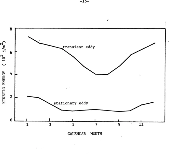
1.1 Distribution of kinetic energy of transient and stationary 15 eddies for different months. (from Oort and Peixoto, 1974)
1.2 Conversion of zonal available potential energy to transient 16 ( C1(PMPTE) ) and stationary ( C1(PM,P SE) ) eddy available
potential energy for different months. (from Oort and Peoxoto, 1974)
1.3 Spectra of eddy kinetic energy ( K ) and conversion of 17 zonal available potential energy to eddy available
potential energy ( C1 ). (from Tenenbaum, 1976)
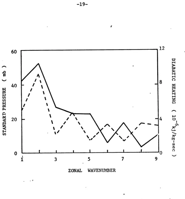
1.4 Spectra of standard pressure amplitude due to surface 19 topography and diabatic heating. (from Derome and
Wiin-Nielsen, 1971)
1.5 Normalized spectrum of transient eddy kinetic energy at 20 50 N, 500 mb, in winter. (from Julian et al, 1970)
1.6 Magnitude of conversion of kinetic energy from wavenumber 25 m to n, summed from m=1 to 30 in winter, I CK(m/n) .
(from Tenenbaum, 1976)
2.1a Horizontal geometry of j -plane model. 30 2.1b Vertical geometry of A -plane model.
2.2 Critical shear of the 2-level model as a function of 36 zonal wavenumber.
2.3 Barotropic zonal flow ( (U-0/4 ) as a function of 37
for Rossby waves of wavenumbers 2, 4, 6.
2.4 Zonal shear ( 1; /A ) as a function of 8T/6 for Rossby 38 waves of wavenumbers 2, 4, 6.
2.5 Barotropic zonal flow ( (U- / ) as a function of zonal 41 wavenumber ( K ) of Rossby wave, for zonal shear tU v-O
and T PSI. Both baroclinic and barotropic modes are
shown.
2.6 Amplitude ratio (8 B8 ) as a function of zonal wavenumber 42
( K ) of Rossby wave, for zonal shear rlP=.
2.7 Comparison of phase speeds of Green modes obtained with 45 a high vertical resolution model and phase speeds of neutral baroclinic Rossby waves in a two-level model.
-9-Figure Page
2.8 Vertical structure of streamfunction phase for the 46 fastest growing Green mode in a high vertical resolution
model.
3.1 Effects of friction on stationary wavenumber two forced 54 by topography.
3.2 Effects of friction on stationary wavenumber two forced 55 by diabatic heating.
3.3 Calculated stationary eddy heat flux as a function of 56 longitude and latitude for winter.
3.4 Observed stationary eddy heat flux as a function of 57 longitude and latitude, averaged over January 1973,
1974 and 1975.
3.5 Calculated and observed zonally averaged stationary eddy 59 heat transport for winter, as a function of latitude.
3.6 Calculated spectra of northward stationary eddy heat 60 transport and correlation coefficient.
3.7 Calculated spectra of energy conversions of stationary 63 waves in winter.
5.1 Contours of constant growth rate ( 1J ) of most 84 unstable mode for planetary scale basic wave with
non-dimensional wavenumber 1'Ik =3.9, and lowest truncation. 5.2 Grbwth rate ( - I ) and zonal shear ( 2. ) for lowest 86
truncation along baroclinic, barotropic and mixed baroclinic-barotropic paths, for most unstable mode.
'-k.
=3.95.3 Spectra of barotropic and baroclinic perturbation wave 88 amplitude ( ~X~ , |Y ) for the most unstable mode and
its meridional wavenumber ( L L ). . i0 =3.9
5.4 Kinetic energy and heat transport spectra ( K(n), v'T'(n) ) 91 for the most unstable mode. t-Ik =3.9
5.5 Energetics of the most unstable mode. IIk =3.9 92 5.6 As in Fig. 5.1 but for very large scale basic wave. 94
.A nt=1 0
-10-Figure Page
5.8 As in Fig. 5.3 but for
PIk
=10. 975.9 As in Fig. 5.4 but for
iHk
=10. 985.10 As in Fig. 5.5 but for
rlk
=10. 995.11 As in Fig. 5.1 but for synoptic scale basic wave. 101
r/k
=1.2
5.12
As in Fig 5.2 but for
rIL
=1.2.
102
5.13 As in Fig.5.3 but for
lk-
=1.2. 1035.14 As in Fig.5.4 but for
'I4k
=1.2. 1045.15 As in Fig.5.5 but for
tlk
=1.2. 1076.1 Growth rate of most unstable mode as function of wave 129 amplitude and meridional wavenumber. Basic wave is
wave-number one and zonal shear flow is near minimum critical shear.
6.2 Spectra of jXI , JYI , K(n) and v'T'(n) of all unstable 130
n n
modes of meridional wavenumber L /k = 5. Also shown are
the energetics and correlation coefficient for heat transport. Parameters of basic flow as in Fig. 6.1.
6.3 Observed wavenumber spectra of meridional sensible heat 133 flux for stationary and transient eddies, at 850mb, 60ON
in winter. (from Kao and Sagendorf, 1970)
6.4 Kinetic energy and heat transport spectra, energetics and 134 correlation coefficient for heat transport for most unstable even and odd perturbations. Basic wave is wavenumber two and zonal shear flow is near minimum critical shear.
-11-Table Page
1.1 The four major kinds of atmospheric eddies and their 21 likely sources, and the amounts of kinetic energy and
conversion of zonal available potential energy to eddy available potential energy, on an annual basis. (from Stone, 1977)
3.1 Sensitivity of forced stationary waves to variations of 67 the friction coefficient, meridional wavenumber and
diabatic heating.
5.1 Non-dimensional growth rate and meridional wavenumber for 118 most unstable mode calculated from a second order expansion valid for the Lorenz regime, together with the exact
values.
5.2 As in Table 5.1 but the second order expansion is valid 120 for the Kim regime.
-12-I. INTRODUCTION
Examination of time mean weather maps reveals the existence of perturbations(deviations from axial symmetry) of considerable amplitude. The existence of disturbances after time averaging suggests excitation by geographically fixed sources. The primary sources of such disturbances are (i) deflecting effects of mountain ranges on zonal currents and
(ii) heating by a steady distribution of heat sources and sinks. The forcing of stationary waves by either topography (e.g. Charney and Eliassen, 1949) or diabatic heating (e.g. Smagorinsky, 1953) has fre-quently been discussed in the literature. Investigations including both forcing mechanisms have also been done (e.g. Derome and Wiin-Nielsen, 1971). Daily weather maps also show the existence of perturbations of comparable amplitudes with much shorter time scales, typically of the order of several days. These transient waves have conventionally been attributed to baroclinic instability of the zonal current (Charney 1947. Eady,1949).
In order to better understand the stationary and transient compo-nents of atmospheric wave motions, the wind and temperature fields are often decomposed into the mean, stationary and transient components as follows: consider any field, such as meridional veolcity 4 . Then
L It
where
3
X and " I are zonal and time means respectively; asterisks and primes denote deviations from the zonal and
-13-time means respectively. The -13-time and zonal mean of a quadratic quan-tity such as meridional heat transport can be written in the following
form (
T
denotes temperature).
[
T
1
[ [71
+
Ij+
(ST
The terms on the right hand side are referred to as the zonal mean ( Z ) component; the stationary eddy (SE) component and the transient eddy
(TE) component respectively.
Holopainen (1970) examined the energetics of stationary waves by evaluating the various terms in the equations of balance of kinetic energy (KE) and available potential energy (APE) using observational
statistics. Only those processes which affect the energy of stationary waves were considered. He found the dominant conversions in winter are ZAPE --- SEAPE ---- SEKE, characteristic of atmospheric eddies
generated by baroclinic instability of the zonal flow. Dissipation was found to be much more important than topographic forcing, SEAPE was destroyed by diabatic heating and the primary energy source of the
stationary waves was ZAPE. Holopainen concluded that stationary dis-turbances are essentially free standing or slowly moving baroclinic waves, which need external forcing in order to occur on time-mean maps. He suggested the simplest model which would approximately produce the
observed energetics of stationary waves was a baroclinic model with diabatic forcing as the only forcing mechanism.
Stone (1977), from physical considerations and observational evi-dence, classified atmospheric eddies into four major types: baroclinic and non-baroclinic SE's; and planetary scale and synoptic scale TE's.
-14-The classification of SE's is based on the observation that summer SE's do not transport heat poleward while winter SE's do, and that the winter SE energy cycle is dominated by baroclinic conversions while that in the summer is not. Figs. 1.1 and 1.2, taken from the results of Oort and Peixoto (1974), show the distribution of TEKE and SEKE, and the conver-sions of ZAPE to TEAPE and SEAPE by the dominant horizontal processes for different months, respectively. In both winter and summer, SE's account for about 20% of the total eddy KE, but the conversion ZAPE---SEAPE is about 50% of the total conversion in winter and almost 0% in summer. Also in winter the conversion SEAPE---)SEKE is the main source of SEKE (Holopainen, 1970). Since these conversions in winter imply strong poleward and upward transports of sensible heat, we see there is a strong baroclinic component in the SE's giving rise to
efficient heat transporting waves in winter, The summer SE's transport almost no heat and are termed non-baroclinic. The non-baroclinic SE's are likely due to topographic forcing, as topographically forced waves do not transport heat (Derome and Wiin-Nielsen,1971).
Stone's classification of the TE's was based on spectral analysis. Fig. 1.3 shows the eddy KE and the conversion ZAPE -EAPE as a func-tion of the zonal wavenumber in January, taken from Tenenbaum (1976). There are two peaks in both spectra: a primary peak at planetary scales
(wavenumber 1-3) and a secondary peak at synoptic scales (wavenumbers 5-8). The presence of two peaks indicates at least two different phy-sical processes are at work generating eddies in January. The topo-graphic and diabatic forcings have similar spectra as both are prima-rily determined by the distribution of oceans and continents. Their
-15-4L 0-% 04 0 o r-4 z z I.-' I-eddy stationary eddy 0 I I I I 1 3 5 7 9 11 CALENDAR MONTH
Fig. 1.1 Distribution of kinetic energy of transient and stationary eddies for different months. (from Oort and Peixoto, 1974)
-16-1.5 C (pPTE (N 1.0
0.5
C (P 9P S) 0 1 3 5 7 9 11 CALENDAR MONTHFig. 1.2 Conversion of zonal available potential energy to transient ( C1(PMPTE) ) and stationary ( C1(PMPSE) ) eddy available potential energy for different months. (from Oort and Peixoto, 1974)
1.5 I -0.8 1 .5 -% - 0.6 SI K 0.2 0.4 1 3 5 7 9 11 13 15 WAVENUMBER
Fig. 1.3 Spectra of eddy kinetic energy ( K ) and conversion of zonal available potential energy to eddy available potential energy ( C 1 ), (from Tenenbaum, 1976)
-18-spectra, taken from Derome and Wiin-Nielsen(19 71), are shown in Fig. 1.4. As planetary scales are dominant in these forcings, it is natural to associate the planetary scale peak in the observed spectra of Fig. 1.3 with these forcings. One would expect these forcings to give rise to
SE's, but the planetary scale waves must also contain a substantial TE component: if we attribute all of the KE and conversion in wave-numbers four and higher to TE's, the partitioning of the total eddy KE and of the total baroclinic conversion ZAPE )EAPE (see Figs. 1.1 and 1.2) still implies that at least half the KE and conversion in the planetary scales (wavenumbers 1 to 3) are due to TE's. That there is a lot of KE in planetary scale TE's is shown in Fig. 1.5, taken from
Julian et al (1970). We see that a significant portion of TEKE in winter lies in the planetary scales. The synoptic scale TE's may be attributed to baroclinic instability, since their scale and structure are close to those of the dominant modes given by baroclinic instability theory.
Table 1.1 summarizes the four kinds of eddies classified by Stone (1977) with their likely sources, and estimates of the partitioning among them of the total KE and the total baroclinic conversion ZAPE--EAPE on an annual basis. As we discussed earlier, the synoptic scale TE's and non-baroclinic SE's are likely due to baroclinic instability and topographic forcing respectively. The planetary scale TE's may also be associated with baroclinic instability, as their properties are similar to those of synoptic scale TE's, except for the different zonal scale. Their scale may be determined by external forcing such as dia-batic heating.
The source of baroclinic SE's is unclear. Stone (1977) observed that planetary scale TE's and baroclinic SE's may be different
mani- -19-60 40 20 0 H H H z 0 O I Cl I o 1 3 5 7 9 ZONAL WAVENUMBER
Fig. 1.4 Spectra of standard pressure amplitude due to surface topography ( solid line) and diabatic heating ( dashed line). (from Derome and Wiin-Nielsen, 1971)
2
00
1 3 5 , 7 9 11 13 15
WAVENUMBER
Fig. 1.5 Normalized spectrum of transient eddy kinetic energy at 50N, 500 mb, in winter. ( from Julian et al, 1970)
4 4
Table 1.1 The four major kinds of atmospheric eddies and their likely sources, and the amounts of kinetic energy ( K ) and conversion of zonal available potential energy to eddy available potential energy ( C1 ), on an annual basis. (from Stone, 1977)
EDDY TYPE KE C1 SOURCE
Synoptic-scale TE's 45% 40% Baroclinic instability
Baroclinic instability
Planetary-scale TE's 35% 30% initiated by external
forcing ?
Non-baroclinic SE's 10% 0% Topographic forcing
Baroclinic SE's 10% 30% Baroclinic instability
-22-festations of a single phenomenon - eddies generated by a cooperation between diabatic heating and baroclinic instability. Such eddies would be of planetary scale and baroclinic in nature, and could contain both TE and SE components. A relation between baroclinicity and diabatic forcing is also suggested by the work of van Loon and Williams (1976). They examined records of temperature and sea level pressure from 1900
-1972 and found that the period 1900 - 1941 was a warming period, during which the average temperature of the Northern Hemisphere increased, while the period 1942 - 1972 was a cooling period. They also found poleward transport of sensible heat by SE's took place in preferred longitude intervals on the front and rear sides of the Icelandic and Aleutian lows. A larger poleward flux in high latitudes during the warming period was found to be connected with a stronger meridional circulation, hence stronger baroclinicity, around the Icelandic low and on the east side of the Siberian high than during the cooling period. The lows and highs are in part diabatically forced, thus their results suggest that stronger baroclinicity coupled with diabatic heating gave rise to a larger SE heat transport.
Yao (1977) examined the maintenance of quasi-stationary waves by using a 2-level quasi-geostrophic spectral model on a A -plane. Diabatic heating was in the form of Newtonian cooling with an imposed
thermal equilibrium temperature profile which varied only with latitude. Surface friction and topography were present at the bottom boundary. Topography of wavenumber n in the zonal direction and first mode
in the meridional direction was used to force the quasi-stationary waves. The model's motion allowed for zonal wavenumbers 0, n, 2n and the first
-23-three modes in the meridional direction. The cases n = 2,3 were con-sidered. The stationary solution was perturbed to find the quasi-equilibrium state. If the flow is not highly irregular, APE of the quasi-stationary waves was maintained by the conversion ZAPE---SEAPE. For n = 3 and moderate values of the imposed thermal equilibrium
temperature gradient (
~Te )
and the internal frictional dissipative time scale (k
1 ) , KE of these waves was maintained by theconversion SEAPE---- SEKE. For smaller values of
AT
or , KE was supplied to the quasi-stationary waves by the conversion ZKE---4SEKE through the topographic forcing. The former case, characterized by the baroclinic conversions ZAPE --- SEAPE---- SEKE, is like the atmospheric winter regime when strong baroclinicity results due to the large pole-to-equator temperature gradient. Yao's results suggest that, in this case, the quasi-stationary waves are generated by baroclinic instability together with external forcing (topography); the latter is required to generate zonal thermal variations and hence SEAPE. Thus baroclinic instability and external forcing may work together to generate the baroclinic, efficient heating transporting SE's observed in winter.
Consideration of Holopainen's (1970), Stone's (1977) and Yao's (1979) works suggests tha hypothesis that the efficient heat transport by SE's in winter is due to instability of a baroclinic flow with exter-nal forcing. The exterexter-nal forcing will force SE's and the resulting zonal flow and SE field will be unstable to small wavelike perturbations. As the basic flow is non-axisymmetric, interaction between the basic wave and the perturbation will generate further waves, i.e. a spectrum
-24-scale waves, such eddy-eddy interactions are in fact observed. Fig. 1.6, taken from the results of Tenenbaum (1976), shows the winter conversion of KE from wavenumber m to n , summed from m = 1 to 30, as a function of n . We see there are two peaks in the spectrum, in the planetary and synoptic scales. For the planetary scale peak at n = 3, the magnitude of this conversion is about 25% that of the conversion ZAPE---EAPE (Fig. 1.3). Thus eddy-eddy interaction is by no means negligible compared to eddy-mean flow interaction for these waves. For our hypothesis, the heat transport spectrum obtained as a result of eddy-eddy interaction will be of particular interest.
As a first step in examining our hypothesis, we will evaluate the heat transport and energetics of stationary waves forced by realistic topography and diabatic forcing in winter. The model used is similar to that of Derome and Wiin-Nielsen(1971). They examined forced sta-tionary waves in mid-latitudes in winter but did not calculate their heat transports. We will find that the efficient heat transporting winter stationary eddies are not adequately modelled, and this will
lead us to our next step, the study of the stability of a baroclinic Rossby wave in a zonal flow with shear. This problem will be the main
subject of this thesis. The Rossby wave is a free wave and must satisfy a dispersion relation. For realistic profiles of the zonal flow, this constraint means that the waves are generally propagating relative to tht earth. Thus the free Rossby wave connot be identified with a forced stationary wave. However, the scale selection mechanism discussed above still operates. In particular, if realistic kinetic energy and heat transport spectra in the planetary scales are obtained with a planetary scale Rossby wave in the basic flow, studies of the stability of forced
-25-0.2 C%4 0.1
0
I I I I i 1 3 5 7 9 WAVENUMBERFig. 1.6 Magnitude of conversion of kinetic energy from wavenumber m to n, summed from m=l to 30 in winter, C [K(m/n)l
-26-planetary scale waves will be justified.
The study of the stability of free planetary scale Rossby waves is of great interest aside from any insight it may give for the problem of the stability of stationary waves. In Chapter II, we will show that the neutral baroclinic Rossby wave in the 2-level model can be identified with slowly growing longwave modes, first discovered by Green (1960). Although these modes have small growth rates, they can attain large amplitudes. Gall (1976), in a numerical study using a
general circulation model, examined the baroclinic instability of realis-tic zonal wind profiles. He found that long, deep baroclinid waves do attain much greater amplitudes than short, shallow waves. This is because the stabilizing effect of nonlinear wave-mean flow interaction occurs most rapidly in low levels and thus the short, shallow waves are affected more by non-linear effects. The "Green modes", being long, deep waves, can thus grow to finite amplitude. This is one possible
source for the kinetic energy observed in planetary scale TE's. Whatever their source, these finite amplitude waves will affect the nature of the baroclinic stability problem. Thus from the point of view
of having as realistic a basic state as possible, the stability of planetary scale Rossby wave is of interest in its own right.
The stability analysis of a non-axisymmetric basic state is also of importance because it provides a mechanism for selecting meridional scales. Simple models of baroclinic instability of a zonal flow (Charney 1947, Eady 1949, Phillips 1954) do not have any selection mechanism for the meridional scale of unstable baroclinic waves, as the most unstable mode has an infinite meridional scale. This difficulty is usually avoided
-27-by placing walls at fixed latitudes so that the meridional scale is equal to this forced geometric scale. This artifice is unrealistic as there are no walls in the atmosphere. The meridional scale is also of crucial importance in finite amplitude dynamics of baroclinic waves. In Pedlosky's (1971) analysis of finite amplitude baroclinic instability is a 2-layer system with small dissipation, the meridional scale appears explicitly in the steady state wave amplitude. Studies by Kim (1975) and Pedlosky (1975a)have illustrated in two particular cases that the presence of a basic state wave leads to the selection of a finite meri-dional scale, in both cases of the order of the radius of deformation. Thus we will be particularly interested in examining the meridional scales selected in our stability analysis.
The stability of our basic flow to small perturbations will be examined using linear theory. The stability of non-axisymmetric flows has frequently been discussed in the literature. Lorenz (1972) examined the stability of the barotropic Rossby wave and applied the results to atmospheric predictability. Gill (1974) examined the same problem and identified Rayleigh instability and resonant triad regimes depending on the ratio of interial to A -effects. Kim (1975) investigated
the stability of the baroclinic Rossby wave as a means of generating ener-getic eddies in the ocean. These studies have no vertical shear in the zonal flow. For the investigation of our hypothesis, this is an
unrealistic approximation as the zonal shear represents an important
energy source for instabilities. Pedlosky (1975a)considered the stability of a baroclinic wave and a zonal flow at neutral stability as a mechanism for selection of meridional scale of motion. Merkine and Israeli (1978)
-28-examined the stability of a stationary Rossby wave in a baroclinic zonal flow and applied the results to mountain induced cyclogenesis. Pedlosky's (1975a)basic wave is of synoptic scale and small amplitude. In Merkine and Israeli's (1977) study, the basic wave is of synoptic scale and the meridional wavenumber of the perturbation is fixed at one value. In our parameter study of the stability of Rossby waves in a baroclinic zonal flow, the basic wave will be of arbitrary scale with arbitrary amplitude; the meridional wavenumber will also be allowed to vary.
Chapter II presents the basic formulations of a 2-level quasi-geostrophic, mid-latitude P -plane model together with some exact, free solutions. The energetics and heat transport of SE's forced by realistic topography and diabatic heating are examined in Chapter III. Chapters IV and V present a parameter study of the stability of a Rossby wave in a baroclinic zonal flow. We present in Chapter VI some appli-cations to the atmosphere, and the conclusions in Chapter VII.
-29-II. BASIC FORMULATION
II-1. Basic equations in a two layer atmosphere
The synoptic and planetary scale waves of mid-latitudes can be described by the quasi-geostrophic system of equations. We assume the motion takes place in a cyclic zonal channel of width Yo in the
y-direction and of length X0 in the x-direction. The Coriolis parameter is assumed to have a constant meridional gradient, ,
to take into account sphericity of the earth (Fig. 2.l.a). The governing equations in pressure co-ordinates are:
P
(2.1)
7p (2.2)+
RT
TP
f-"
J(Js~ (2.3)(2.4)
In the above, t is time, p pressure,
T(,
9)
-the horizontal Jacobian, 4Z o + where 1o is the Coriolis parameter at 45*N,
*
the geostrophic streamfunction for thehorizontal flow, ()= the vertical velocity,
T
the temperature, 1 the specific heat capacity at constant pressure, . the gasconstant, -( - the static stability, S the
horizontal divergence and H the diabatic heating due to ocean-land contrast.
-30--l
1
y-
2 YO x=0 x=X0(a)
p = 0 mb p = 250 mb p2= 500 mbtf.
p3= 750 mb p 4= 1000 mb(b)
Fig. 2.1 ( a ) Horizontal geometry of -plane model. ( b ) Vertical geometry of
P
-plane model.- plane
-31-The horizontal velocity field is geostrophic:
V
" X where is a unit vector in the vertical direction. The staticstability is assumed to be constant. Equations (2.1)-(2.4) are the
quasi-geostrophic vorticity equation, the thermodynamic equation, the hydrostatic equation and the continuity equation respectively. The boun-dary conditions are:
4=
0O
at l+0=0 at
p0
, the top of the model atmosphere'j-
atPs
, the bottom of the model atmosphereis the geostrophic vorticity and quantities with subscript
denote values at the bottom of the atmosphere. The first contribution to the surface vertical velocity is due to flow of air over surface topo-graphy where the standard pressure is ? . The second contribution
is due to viscosity in the Ekman layer which is taken into account by
the use of a friction coefficient F , forcing a surface vertical velocity which balances Ekman convergence (Charney and Eliassen, 1949).
In the vertical direction, the atmosphere is divided into tow layers of equal mass. As shown in Fig. 2.1b, we carry , 8 at levels 1 and 3; T , C) at level 2 and () at the top and bottom of the atmosphere. Applying Eqs. (2.1) and (2.4) at levels 1 and 3, Eqs. (2.2) and (2.3) at level 2 and using linear interpolation for , we have
-32-(2.5)
T (2.6)
'31
T
(2.7)The boundary conditions become
4
,o
1' . 0
9at
yoi
oA
3 o
at pMo
p, -P.
- PF
at
Linear extrapolation is used to give -g 4L(k" ,) in the frictional component of the surface vertical velocity. It can be shown that
V
, rather than an extrapolated \ , must be used in the topography component so that topography does not make a net con-tribution to the time rate of change of total energy.We introduce the mean and thermal streamfunctions = 2j I ,
44 z *A " 3 . Adding and subtracting Eqs. (2.5) and (2.6) and
rewriting in terms of and
'1
, we getatv14
3(++", '4f
T
+V)
,
'-
L
,
,-o
(2.8)
,
,,
(,
) + j(4I
.f)2-
,). o
),-
-33-Eliminate W. between Eqs. (2.9) and (2.7) and let ( ,' is the radius of deformation). We then obtain
%2t
s
3(k
-F')+
'L,
+J(4
(
-t
i
)
J((,itf)
f
+D
+L
-
+
+
o
(2.10).Equations (2.8) and (2.10), together with the appropriate boundary condi-tions, are the equations of interest.
In order to derive an energy equation for an adiabatic and friction-less atmosphere, it is more convenient to write Eqs. (2.8) and (2.10) in the following form:
i.)O
•(2.11)
I
J+
J
11
)4
') JT.F4S)-i ?1)-
(2.12)The above equations express each layer, with the effect Multiplying Eq. (2.11) adding, we get
the conservation of potential vorticity for of surface topography in the lower layer. by ' and Eq. (2.12) by
'
andit-~ (KE, + PC,) -
(Kel PEI)
I~t~
+
t,-,
,$np
+~
1
ZL
.
-where + J( ; ) is the material derivative, Ej
=
( s+C
,is the kinetic energy and
PE,-
L ," "P
E
is the potential energy for each layer ( -1,1 ) . For a bounded atmosphere with zero
-34-normal velocity on the boundary, integration of Eq. (2.13) shows that the total energy of the bounded atmosphere is conserved:
.
j
(
+E,
IKE+
P,
+?E, )
4Y
=0
11-2. Free solutions of the basic equations
In the absence of friction, topography and diabatic forcing ( Wq.O= ) solutions to Eqs. (2.8) and (2.10) exist of the form
f
-UI + 8iY
k(Y-ct)
(2.14)
(2.15)
This solution describes zonally propagating Rossby waves in a zonal flow. Because of its simple structure, it is an exact solution to the governing nonlinear equations. The resulting diapersion relation is
al (e+ I) (2.16)
The ratio of wave amplitudes is also determined:
- (- -)) -2 17)
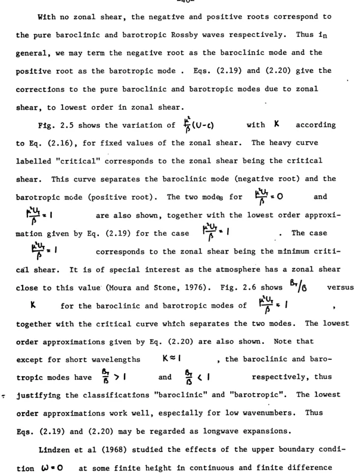
-35-For the Rossby waves to be non-growing, C must be real. This in turn requires the zonal shear not to exceed the "critical shear" for
the 2-level model:
-P AhI{&CAI (2.18)
This is shown in Fig. 2.2. The short waves (
I4
K ) do not have a critical shear and are always stable. However, the 2-level model is not really valid at such short wavelengths. Analysis of continuous analog of the 2-level model (Green, 1960) shows that the critical shear expres:-d by Eq. (2.18) actually represents a transition between condi-tions where the dominant unstable waves are long, deep waves and condicondi-tions where the dominant unstable waves are short, shallow waves. The 2-level model is capable of resolving only the former unstable modes. Held (1978), using scaling arguments, has shown that the vertically integrated kinetic energy and eddy sensible heat flux of a baroclinic wave are proportional to the cube of the wave height. Thus the long, deep waves, which are resolved by the 2-level model, are much more efficient at transporting heat poleward than the short, shallow waves.Eqs. (2.16) and (2.17) provide two equations for the four quantities
(U-)
,K
and . The first two describe the zonalflow while the last two describe the Rossby wave. Specifying any two of these four quantities determine the other two, with an overall wave amplitude being arbitrary. In Figs. 2.3 and 2.4, we show the variation of the zonal flow for different wave properties, i.e., variation of
-36-0 0.2 0.4 0.6 0.8 1.0
ZONAL WAVENUMBER ( K=k/ )
Fig. 2.2 Critical shear of the 2-level model as a function of zonal wavenumb er. 10 8 6 r-q U
VI
*r4 -I u4 2 04 4 16 14 12 wavenumber 2 10 8 6 -wavenumber 4 4 2 - wavenumber 6 0 0.01 0.1 1 8T/8 10 100
Fig. 2.3 The barotropic zonal flow ( (U-c)) as a function of
/e for Rossby waves of wavenumbers 2,4,6. The dashed
curve represents critical conditions for different
wavenumbers.
4 4
7-I I
6
I I wavenumber 25
I I I4
I I I3a
I 002
1.
0
0.01
0.1
1
10
100
Fig. 2.4 The zonal shear ( ~ ) as a function of /6 for Rossby
waves of wavenumbers 2,4,6. The dashed curve represents
-39-different values of K . The three values of K shown
corre-spond to wavenumbers 2,4,6 at midlatitudes. The value of the ordinate
at the critical condition given by Eq. (2.18) for each wavenumber is
shown by the dashed lines. Note for our choice of 86 and K as independent variables, the ordinate is a single-valued function of the abcissa. We see that for each wavenumber, the zonal shear is bounded by the corresponding critical shear, in order that the wave be stable to small perturbations. In the limits 0and
--( ) and (U- ) respectively, while
S--
for both limits. These are the limiting pure barotropic and pure baroclinic Rossby waves respectively. Dimensionally, they aredescribed by
R
,o
,
U- =
c-
I
and
0 ,U-c(-
c
I',respectively, and both have VI = . For non-zero values of the zonal shear, the wave consists of both barotropic and baroclinic components.
Condition (2.18) is identical to the condition for convergence of the expansion of the radical in Eq. (2.16). Thus for stable waves, we have from Eq. (2.16) for the negative and positive roots:
I %, .
j
1u-
)--
)(2.19)
- K0-0
while Eq. (2.17) gives
( *)(2.20)
K O-K
-40-With no zonal shear, the negative and positive roots correspond to the pure baroclinic and barotropic Rossby waves respectively. Thus in general, we may term the negative root as the baroclinic mode and the positive root as the barotropic mode . Eqs. (2.19) and (.2.20) give the corrections to the pure baroclinic and barotropic modes due to zonal shear, to lowest order in zonal shear.
Fig. 2.5 shows the variation of t(UJ-) with K according to Eq. (2.16), for fixed values of the zonal shear. The heavy curve labelled "critical" corresponds to the zonal shear being the critical shear. This curve separates the baroclinic mode (negative root) and the barotropic mode (positive root). The two modes for 1 0 and
- I are also shown, together with the lowest order approxi-mation given by Eq. (2.19) for the case " . The case
I=
corresponds to the zonal shear being the minimum criti-cal shear. It is of special interest as the atmosphere has a zonal shear close to this value (Moura and Stone, 1976). Fig. 2.6 shows BT/6 versusK for the baroclinic and barotropic modes of ,
I
together with the critical curve which separates the two modes. The lowest order approximations given by Eq. (2.20) are also shown. Note that
except for short wavelengths K I , the baroclinic and
baro-tropic modes have and ( respectively, thus
justifying the classifications "baroclinic" and "barotropic". The lowest order approximations work well, especially for low wavenumbers. Thus Eqs. (2.19) and (2.20) may be regarded as longwave expansions.
Lindzen et al (1968) studied the effects of the upper boundary condi-tion W.)O at some finite height in continuous and finite difference
-41-10 5 barotropic baroclinic X x 0 0.2 0.4 0.6 0.8 1 ZONAL WAVENUMBER ( K )
Fig. 2.5 P-c) J as a function of zonal wavenumber ( K ) of Rossby wave, for zonal shears "/ 0O0 (dashed) and to 5=t
(solid). Both baroclinic and barotropic modes are shown. Crosses denote lowest order approximation for the case
PUr -MI . Heavy curve corresponds to critical conditions
-42-10 5 X baroclinic X 1 0.5 0.5 rbarotropic 0.1 0 0.2 0.4 0.6 0.8 1 ZONAL WAVENUMBER ( K )
Fig. 2.6 /8 as a function of zonal wavenumber (
K
) of Rossby wave, for zonal shear P I . Crosses denote lowest order
-43-models of free and forced linear oscillations. Their basic atmosphere was rotating, isothermal and quiescent. Comparisons with results obtained from an unbounded atmosphere with the radiation condition or boundedness as upper boundary condition indicated spurious oscillations were generated due to reflection at the upper boundary. In particular, for the 2-level model, the only non-spurious free oscillation was found to be the pure barotropic Rossby wave. However, Charney and Drazin (1961) showed that stationary, small amplitude, adiabatic and quasi-geostrophic waves in a uniform zonal flow can propagate energy vertically only when the zonal flow is westerly and less than some critical velocity. Thus the use of realistic atmospheric zonal winds, instead of the resting basic state used by Lindzen et al (1968) may prevent forced waves from reaching the upper boundary. Kirkwood and Derome (1977) investigated this problem
by examining the forced wavenumber 1 response in a high resolution reference model (200 vertical levels) with radiation condition at a finite height as upper boundary condition, and a layer model (101 to 6 levels) with the upper boundary condition W)=O at pa O (the P model). Realistic vertical zonal wind profiled for different seasons, together with New-tonian cooling which varied with height and which had a maximum at 50 km, were used. For winter, it was found that the strong upper level westerlies acted as a reflecting medium and results of the sufficiently high resolu-tion P model agreed well with those of the reference model. In other words, as long as the upper level westerlies were resolved, the rigid lid upper boundary condition did not have much effect as little energy was able to penetrate up to that level anyway. For spring, the week, westerly zonal winds did not inhibit the vertical propagation of energy, but the damping effect of Newtonian cooling prevented the wave from reaching the
-44-top boundary with significant amplitude. Thus the P model with adequate resolution again minimized the effects of the upper rigid lid.
Our model has only two vertical levels and is not able to model the stratospheric westerlies or the Newtonian cooling maximum. However, the use of a rigid lid as an upper boundary condition may be thought of as a strongly reflecting or dissipative winter stratosphere. Indeed, more refined calculations than the 2-level model have shown the existence of the counterpart of the baroclinic Rossby wave of the 2-level model. Fullmer (1979) examined the baroclinic instability of one dimensional basic states using a s-plane quasi-geostrophic model. His model had 48 levels in the vertical with the troposphere extending from 1000 to 250 mb and the stratosphere from 250 to 0 mb. The upper boundary condi-tion used is vanishing perturbacondi-tion streamfunccondi-tion amplitude at the top of the model atmosphere. Slowly growing, long wave modes, first dis-covered by Green (1960), were found using a basic state with the static
stability of the stratosphere fifty times of the troposphere and a linear shear zonal wind which vanished at the ground and reached 24 m/sec at 250 mb, The ratio of static stabilities of the stratosphere and tropo-sphere is realistic for mid-latitude winter conditions; the zonal wind profile is also realistic in the troposphere. The doubling time of the . "Green modes" is over 10 days. Fig. 2.7 shows the phase speed of these modes as a function of zonal wavenumber, together with the phase speed of the baroclinic Rossby wave in the 2-level model with the corresponding values of tropospheric static stability and barotropic and baroclinic zonal flow components. We see that the phase speeds agree well for long wavelengths. The vertical structure of the streamfunction phase for the fastest growing Green mode is shown in Fig. 2.8. There is an abrupt
-45-15 10 S5L 1 2 3 4 ZONAL WAVENUMBER
Fig. 2.7 Comparison of phase speeds of Green modes obtained with linear vertical shear of basic zonal wind and stratospheric static
stability fifty times that of the troposphere ( o ; from Fullmer, 1979), and phase speeds of the neutral baroclinic Rossby wave in the two level model with comparable basic flow parameters
-46-0 200 400 a 600
800
1000 2 4 21 PHASE ( radians )Fig. 2.8 Vertical structure of streamfunction phase for the fastest growing Green mode. Basic flow parameters as in Fig. 2.7. (from Fullmer,
-47-phase shift of approximately 1T radians at 650 mb, much like the baroclinic Rossby wave which has the upper and lower level streamfunctions out of phase with each other by 180*.
The 2-level model is not able to model the stratosphere but as we discussed earlier, the use of a rigid lid as an upper boundary condition
is analogous to a strongly reflecting or dissipative winter stratosphere. The good agreement of the phase speed and vertical structure of the Green mode in a high vertical resolution model and the baroclinic Rossby wave
in a 2-level model suggests that the latter can be identified with a Green mode.
In this section, we examine the energetics and heat transport pro-perties of stationary waves forced by realistic topography and diabatic
forcing in winter. The latter are taken from Derome and Wiin-Nielsen (1971), hereafter referred to as DWN, who Fourier analyzed Berkofsky and Bertoni's (1955) topographic field and Brown's (1964) heating field. These were shown in Fig. 1.4. DWN found topographically forced waves do not transport heat, while diabatically forced waves transport heat only when friction is present. Quasi-resonance resulted when the zonal scale of the topographic forcing was close to the wavelength of sta-tionary Rossby waves, which are a solution to the unforced problem. Taking winter conditions, the calculated perturbation heights of the 250, 500 and 750 mb surfaces agreed well with observations. Following DWN, we represent the forced stationary waves by Fourier series in the
zonal direction with a sinusoidal meridional structure. The heating
(
H
) , standard pressure due to surface topography ( , ) , meanand thermal streamfunctions (
'
,4 T ) which consist of a zonal flow and forced waves, are expressed as:N
H ti
(
-I
top a
1 -,,
1
L
(Ak'
(3.la)flu
Sl
i(3.1c)
-49-k%
I COAo is the zonal wavenumber, OL and Yo being the radius of the earth and 45'N respectively;X
is the meridional wavenumber, I and I represent linear distance to the east and north respectively. The meridional wavelength is taken to be 60Q latitude. Wavenumbers 1 through 18 are kept in the summation,i.e. N = 18 . Substituting eqs. (3.1) into eqs. (2.8) and (2.10), we obtain upon linearization about the zonal flow a system of algebraic
equations for the amplitudes A
S
Ai and Tvr . It mayfor-mally be written as:
S=
(3.2)where
-
IA
(L
'
4M
J.
and
to-
kl"T,
are the amplitude andphase
of each wavenumber of the diabatic forcing; similarly, .rm,.
I~(
Tand
e, .
(j'
-
are the amplitude and phase of the and O-Tj% '8 'ISO. are the amplitude and phase of the
-50-topographic forcing; 9 - (U-J) _ CL T is a measure
of the vertical velocity forced by topography alone; Rtp6
(u-u,) kW t%
is a measure of the ratio of vertical velocities forced by diabatic heating and topography. Eqs. (3.2) are identical to those solved by DWN, except we have used an energy-conserving extrapolation for thetopographic surface vertical velocity; DWN used an extrapolation obtained from the hydrostatic equation. DWN did not evaluate the heat transport and energetics of the forced stationary waves.
If we assume the determinant of M. does not vanish, i.e. free frictionless Rossby waves are suppressed, then solutions to Eqs.
(3.2) can be written as
(3.3b)
where )N M . Note has dimension of
f/Ui
which is dimensionless. Let
Alt=
hill VVh-4
"I--(d
(M').n)tln
Then-eqs. (3.3) become
-
T
(3.4a)
-51-where
A". MIk
e-o,)BT~.-Uke,
f(.L4LC)4
t6 1h.)
In
the above
i/k.
too,
i
A
and a diabatic component k'. ( I , ) . They are additive because
eqs. (3.2) are linear. Aside from the factor U , all
even in the limit --- , i.e. resonance is not achieved.
Changing the phase of the forcing for a particular wavenumber rotates the vectors
Tr
,_.,
and YT. H and leaves their amplitude unchanged.
-52-The meridional heat transport by the stationary waves is
R
n..
(3.5)
We see that there is non-zero heat transport only if the streamlines tilt with height. For a single wavenumber k, the magnitude of the transport depends on the quantity
where Yr is the angle between JI- and _ . Note A r l
is the absolute value of the correlation coefficient for meridional heat transport; its sign depends on the direction of r. ( _V
it is positive if 14, 1
3J
is along the positive z-direction. As T_, is always parallel to T, , Trl. X T vanishes and thus topographic waves transport no heat. For diabatic waves, I-0(no friction) gives T_ . parallel to 8 , i.e. no heat transport. Thus heat transport by diabatic waves is frictionally
induced. The phase of the forcing does not affect this heat transport, as it depends only on rl , _- and the angle between NV.
and .
In Figs. 3.1 and 3.2, we show the effect of friction on -ave ampli-tude vectors for topographic and diabatic waves for zonal wavenumber 2 and realistic winter values for the other parameters. The phase of the
forcing is 0* and non-dimensional amplitudes are shown. For topographic waves,
2~-X--
-53-Irs is parallel to
Is.
, as noted earlier. Increasing friction decreases the wave amplitude. This is because topographic forcing,like friction, is a surface forcing; thus a large friction implies
topography is negligible and it acts as a purely dissipative mechanism.
For diabatic waves, increasing friction actually increases the wave
amplitude until an asymptotic value is reached. This is due to the
non-surface nature of the diabatic forcing in the 2-level model. A particular value of the friction maximizes I r V I , i.e.
the heat transport; for the values of parameters chosen, this occurs
when
FI
Uk,
~ . However, this may not be realistic in view of the wave amplitude behavior at large friction.In Fig. 3.3, we show heat flux as a function of longitude of
sta-tionary waves forced by realistic topographic and winter diabatic
fields (shown in Fig. 1.4). For comparison, the observed stationary
wave heat flux distribution for the troposphere, averaged over
Janu-ary 1973, 1974 and 1975 is shown in Fig. 3.4. The latter was calculated
from National Meteorological Center (NMC) data at the Goddard Institute of Space Studies. The observed distribution is characterized by three zones of strong northward heat transport: eastern Asia (900E - 150*E), central and eastern Pacific (175*E - 135*W) and eastern North America
and the Atlantic (900W - 10*W). The positions of the first two zones are reproduced well, but the third is displaced about 10* latitude
to the south. The intensity of each zone is modelled poorly: the first
zone is much stronger than observed while the other two are weaker;
agreement is better for the third zone. Areas of large negative (south-ward) heat flux present in themodel calculation are not present in the
-54-0.7 0.1 0.6 110 I I I II I 0.4 I 0.1 0.1 -- ts s I ° 0 0 0.1 0.2 0.3 0.4
Fig. 3.1 Effects of friction (F/Uk2= 0.1,1,10,100) on non-dimensional
topographic wavenumber 2. 2 al rI, denoted by solid line,
UkaLI
,
0,22denoted by dashed line. Parameter values areUp15msec, U =5m/sec, =k, . -12 -2
T 2 P = 3x10 m.
---0,8 10 0.6
-0.4 -
10
/i/ 0.2 u.--
100
1 / I Il I00 1 -0.2 0 0.2 0.4 0.6 0.8 1 1.2 1.4Fig. 3.2 Effects of friction ( F/Uk 2= 0.1, 1, 10, 100) on non-dimensional diabatic wavenumber 2.
UbtH
k
TA-4 denoted by solid line, UCAl1 A.. 4 denoted by dashed line. Parameter values as in Fig. 3.1.4 4 62N 0 0 0 0 0 L 58 4 -1 -3 -1 5 0 0 0 0 0 0 0 0 0 0 0 0 0 20 11 -6 -12 -6 0 A 54 14 -2 -9 -4 15 1631 36 -19 -37 -18 2 T 50 21' -3 -13 -7 23 97 55 -29 -57 -28 2 I 46 22! -4 -14 -7 24 199: 56 -30 -58 -29 2 T 42 15 -2 -10 -5 17 169: 39 -21 -41 -20 2 I IJ U 38 6 -1 -4 -2 7 29 17 -9 -17 -8 1 2 -1 -3 0
6
-3
-10
0
i--101 -5 -15 0 '10' -5 -15 0 7 -4 -11 0 3 -2 -5 00
2
8
0 8 124 1 0 12 137 0 12 138 0 9 '27 0 .4 11 D 34 1 0 0 0 1 3 2 -1 -2 -1 0 E 30N 1 0 0 0 1 3 2 -1 -2 -1 0 0 0 -1 0 0 0 1 0 0 0 0 0 0 1 5E- 25 45 65 85 105 125 145 165 175 155 135 115 95 75' 55 35 15W L 0 N G I T U D EFig. 3.3 Calzulated stationary eddy heat flux as function of longitude and latitude for winter, 11 units of 1017 cal/day/grid point.
* 4 2 3 5 '5 -1 2 0 -3 2 10 2 12 7 54 9 -11 0 0 -4 11 '24' 12 50 -1 -9 1 -2 -2 12 1271 10 46 -11 -3 2 -5 1 9 1311 10 42 -15 3 0 -5 0 6 281 '-j-9 -1 12 i I i -2 5 4 4 -3 8 2 4 18 '481 I I I I -4 8 12 6 -7 4 2 5 22 143 1 1 -4 9 24 -4 9 1301 -1 9 127, L,-J -8 1 1 3 23 '33 -7 0 2 4 20 28 -8 3 5 6 12 4 38 -8 7 -3 -2 1 1 16 5 5 7 19 3 -7 9 9 1 1 -3 34 3 8 -3 0 4 -1 8 8 10 1 12 1 -4 12 11 -2 -1 -1 30N 5 7 -2 -2 0 -1 8 9 7 -3 4 5E 25 45 65 85 105 125 145 165 175 155 3 0 7 9 -2 -1 1 135 115 95 75 55 35 15W L 0 N G I T U D E
Fig. 3.4 Observed stationary eddy heat flux as a function of longitude and latitude, averaged over January 1973, 1974 and 1975. Units are 1017 cal/day/grid point. ( NMC data )
62N 26 -5 -5 6
-58-observed distribution. The latitudes of maximum heat transport agree only for the Asian and Pacific zones. The NMC data are for January only and may not be representative of a typical winter. Haines and Winston (1963) examined the spatial distribution of monthly mean meridional sensible heat flux for a period of 3 1/2 years. They found the poleward heat flux across latitude 450N (wherethe zonally averaged flux is maximum) in winter is dominated by the above zones also. However, for each of the four winters examined, they found the eastern Asia zone to be the most intense, which agrees with our results. The theoretical and observed zonally averaged heat transport are shown
in Fig. 3.5. The latter is taken from Oort and Rasmusson (1971). The transport is underestimated at all latitudes especially poleward of 45"N. The maximum heat transport is about a factor of two smaller than tha observed value and is located about 80 too far south.
The spectra of the northward heat transport ( [Ei
T
] ) and the correlation coefficient ( [ ] IJ' "Jj--]
) ) areshown in Fig. 3.6. For ease of visualisation, absolute values of negative values are shown. The calculated transport is dominated by wavenumber 2. This is not surprising as the forcing is strongest at that scale. The agreement with the observations at 850 mb, 400N is good for wavenumber 1, fair for wavenumber 2 and poor fcr wavenumber 3. The correlation coefficient is generally small ( . 0.5), except for
wavenumbers 8 and 13, which transport almost no heat. The overall corre-lation of the 18 wavenumbers is 0.17. The observed value is 0.59 at 50*N and is above 0.50 in mid-latitudes in winter (Oort and Rasmusson, 1971). Thus the model stationary waves are much less efficient at
IYIILL1- 1UY- -LI*rPYrrul ~
-59-10 observed U Icalculated 0 20N 30 40 50 60 70 80 LATITUDE
Fig. 3.5 Calculated and observed ( from Oort and Rasmusson, 1971 ) zonally averaged stationary eddy heat transport v* T* for winter, as a function of latitude.
A - 1.0 I' I 4 5 A 0.8 4 I - 0 u I I o 0
I
\ 3I \ ' 3 0 -0.6 w , \ o I I I I E2- 4 / 4 0 I I -0.4 / 0 \ I I Go ago0.2
0 L' 0 1 3 5 7 9. 11 13 15 17 ZONAL WAVENUMBERFig. 3.6 Calculated spectra of northward stationary eddy heat transport ( v T I, solid) and correlation coefficient ( e , dashed). Dots indicate negative values. Open