HAL Id: hal-00317208
https://hal.archives-ouvertes.fr/hal-00317208
Submitted on 1 Jan 2004
HAL is a multi-disciplinary open access
archive for the deposit and dissemination of
sci-entific research documents, whether they are
pub-lished or not. The documents may come from
teaching and research institutions in France or
abroad, or from public or private research centers.
L’archive ouverte pluridisciplinaire HAL, est
destinée au dépôt et à la diffusion de documents
scientifiques de niveau recherche, publiés ou non,
émanant des établissements d’enseignement et de
recherche français ou étrangers, des laboratoires
publics ou privés.
systems related to rapid geomagnetic variations
S. V. Apatenkov, V. A. Sergeev, R. Pirjola, A. Viljanen
To cite this version:
S. V. Apatenkov, V. A. Sergeev, R. Pirjola, A. Viljanen. Evaluation of the geometry of ionospheric
current systems related to rapid geomagnetic variations. Annales Geophysicae, European Geosciences
Union, 2004, 22 (1), pp.63-72. �hal-00317208�
Annales Geophysicae (2004) 22: 63–72 © European Geosciences Union 2004
Annales
Geophysicae
Evaluation of the geometry of ionospheric current systems related to
rapid geomagnetic variations
S. V. Apatenkov1, V. A. Sergeev1, R. Pirjola2, and A. Viljanen2
1Institute of Physics, St. Petersburg State University, Ulyanovskaya 1, Petrodvoretz, 198504, St.Petersburg, Russia 2Finnish Meteorological Institute, Geophysical Research Division, P.O. Box 503, FIN-00101 Helsinki, Finland
Received: 13 September 2002 – Revised: 14 March 2003 – Accepted: 12 May 2003 – Published: 1 January 2004
Abstract. To learn about the geometry and sources of the ionospheric current systems which generate strong geomag-netically induced currents, we categorize differential equiva-lent current systems (DEC) for events with strong dB/dt by decomposing them into the contributions of electrojet-type and vortex-type elementary systems. By solving the inverse problem we obtain amplitudes and locations of these elemen-tary current systems. One-minute differences of the geomag-netic field values at the IMAGE magnetometer network in 1996–2000 are analysed to study the spatial distributions of large dB/dt events. The relative contributions of the two components are evaluated. In particular, we found that the majority of the strongest dB/dt events (100–1000 nT/min) appear to be produced by the vortex-type current structures and most of them occur in the morning LT hours, probably caused by the Ps6 pulsation events associated with auroral omega structures. For strong dB/dt events the solar wind parameters are shifted toward strong (tens nT) southward IMF, enhanced velocity and dynamic pressure, in order for the main phase of the magnetic storms to occur. Although these events appear mostly during magnetic storms when the auroral oval greatly expands, the area of large dB/dt stays in the middle part of the auroral zone; therefore, it is connected to the processes taking part in the middle of the magneto-sphere rather than in its innermost region populated by the ring current.
Key words. Geomagnetism and paleomagnetism (rapid time variations) – Ionosphere (auroral ionosphere; iono-spheric disturbances)
1 Introduction
Geomagnetically induced currents (GIC) in long conductor systems, like power transmission systems or pipelines, are caused by rapid changes in the Earth’s magnetic field (e.g. Correspondence to: S. Apatenkov
(apatenkov@geo.phys.spbu.ru)
Boteler et al., 1998; Viljanen and Pirjola, 1994). GICs are driven by the horizontal electric field induced at the Earth’s surface due to time-varying or fast-moving strongly inho-mogeneous ionospheric current systems and affected by the Earth’s conductivity structure. Close correlation between GIC and the time derivative of the magnetic field (dB/dt) has been demonstrated by Viljanen (1998) and Viljanen et al. (2001), so in the present paper we base our analysis of potential GIC candidate events on one-minute magnetic field differences. A large variety of ionospheric current sys-tems exist which differ by their time and spatial scales and motions. Examples of the most intense systems are the eastward and westward auroral electrojets (AEJ), westward travelling surges (WTS), and auroral omega bands (Untiedt and Baumjohann, 1993). The two latter systems have very complicated structures, including a pronounced vortex part. Here and thereafter we discuss the equivalent current systems (ECS), closed completely in the ionosphere, since the real 3-D system of ionospheric and field-aligned currents cannot be uniquely determined by using only ground magnetic field measurements, (Fukushima, 1976), as its curl-free part does not produce any disturbance on the ground.
Until recently, most of the GIC studies concentrated on considering effects of the simplest one-dimensional current system, an east-west aligned auroral electrojet (Albertson and Van Baelen (1970); Boteler et al. (1997); Towle et al. (1992)). However, a recent survey of dB/dt occurrence and their directional distribution (Viljanen, 1997; Viljanen et al., 2001) indicated that many large GIC events display a large contribution from the east-west dB/dt component, es-pecially in the morning LT hours at auroral latitudes, which cannot be explained by AEJ effects. The detailed study of the April 2000 storm by Pulkkinen et al. (2003) also demon-strated the complexity of ionospheric currents during an ex-treme GIC event.
Some attempts have been done to consider more compli-cated geometries of ECS, for example, in model studies of a real power system in works by Viljanen et al. (1999) and Pulkkinen et al. (2000). They concluded that large GIC could
be most probably produced by rapid intensification of AEJ or fast moving WTS. They also discussed the origins of GIC events and found about half of the events to be caused by electrojet variations. However, the rough characterization was based only on the magnetogram shape and is thus not very reliable.
In this paper we address the question of how often is the simple AEJ model adequate for GIC modeling, and, specifically, how large can the contribution from non-one-dimensional systems can be during large dB/dt events. To characterize it in a quantitative way, we represent the equiv-alent currents as a sum of the simplest 1-D (AEJ) and 2-D (vortex) contributions, which allows us to evaluate their rel-ative contributions to magnetic variations observed on the dense IMAGE magnetometer network. With this simple tool we analyse the large dB/dt events observed during the rising phase of the solar cycle (years 1996–2000), and study sta-tistically the spatial distributions and solar wind conditions, paying attention to the relative complexity of the current sys-tem.
2 Quantitative characterization of the equivalent cur-rent systems observed by the IMAGE magnetometer network
In our approach we select the model as simple as possible, using the sum of two basic elementary current systems, a 1-D current (AEJ) and a current vortex. For the AEJ the initial model is that of the linear current aligned perpendicular to the geomagnetic meridian, where geographic components of the magnetic fields are
Bx= µ0I0 2π Hcos γ H2+( ˜x − ˜x c)2 (1) By= µ0I0 2π −Hsin γ H2+( ˜x − ˜x c)2 (2) Bz= µ0I0 2π −( ˜x − ˜xc) H2+( ˜x − ˜xc)2 . (3)
Here, γ is the angle between the geographic and geomagnetic meridians (in our case γ = 14◦), ˜xcis the electrojet position
along the central geomagnetic meridian (referred to the point 67.5◦N, 25◦E, the centre of the IMAGE network, Fig. 1); ˜x
is the location of the observation point (xs,ys) projected to
the central geomagnetic meridian, ˜x = xscos γ − yssin γ ; His the height of the ionosphere assumed to be an infinitely thin layer at 110 km altitude above the Earth’s surface, and
I0is the current amplitude.
To reduce the number of free parameters in this model, the AEJ width is fixed, and assumed to be 100 km. Formally, it is constructed as a sum of 10 line currents of equal amplitude displaced with a 10-km step from each other.
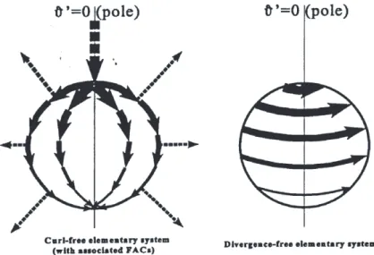
For the vortex we adopted one of two spherical elementary current systems introduced by Amm and Viljanen (1999), namely the divergence-free vortex current (Fig. 2). The
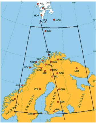
Fig. 1. IMAGE magnetometer stations in 2000. The boundaries of
the grid area for the vortex locations, and the central geomagnetic meridian are also shown.
second curl-free part directly associated with a field-aligned current does not produce any magnetic effect at the Earth’s surface (Fukushima, 1976) and is not of interest for us. The magnetic effect of the divergence-free system is given in spherical coordinates as Br0(r, ϑ0) = µ0I0 4π r 1 q 1 −2r cos ϑR 0 I +( r RI) 2 −1 ! (4) Bϑ0(r, ϑ0) = − µ0I0 4π r sin ϑ0 r RI −cos ϑ 0 q 1 − 2r cos ϑR 0 I +(Rr I) 2 +cos ϑ0 ! .(5)
Here, RI is the ionosphere radius, i.e. RI =RE+110 km; rand ϑ0are the observer’s coordinates in the reference sys-tem with ϑ0=0 at the pole of this elementary current system (see Fig. 2), and I0is the scaling factor.
The contribution of induced currents in the Earth are taken into account using the simple image method. Based on the studies of the Earth’s conductivity structure in Scandinavia (e.g. Viljanen, 1995; Tanskanen et al., 2001), we set a per-fectly conducting layer at a depth of 100 km for the variations with T ∼ 1 min.
All calculations for the vortex part are carried out in a spherical frame of reference which takes into account the Earth’s curvature. The AEJ part is calculated in cartesian
S. V. Apatenkov et al.: Geometry of ionospheric current systems 65
Fig. 2. Two spherical elementary
cur-rent systems used by Amm and Vilja-nen (1999), the curl-free part (left) and the divergence-free part (right). The divergence-free part is used in this study as a model for the current vortex.
geometry for infinite long linear currents. Errors in com-puted magnetic field values caused by discrepancies between directions of geographic and cartesian axes, as well as by the difference between the line current and current aligned along the geomagnetic latitude at H = 110 km at the net-work edges do not exceed 10%.
Our model consists of a sum of previously defined AEJ and vortex current systems, whose positions are set on the grids. The grid for the vortex (Fig. 1) covers 10◦E–40◦E in longitude and 60◦N–75◦N in latitude. The longitudinal step for possible vortex locations is 0.5◦(18–27 km) and the latitudinal step is 0.2◦ (22 km). The latitudinal step for the AEJ model is 50 km and the grid covers 2000 km (41 possi-ble positions) along the central geomagnetic meridian (pass-ing through the point 67.5◦N, 25◦E). This choice of the grid (its steps and boundaries) was decided after experiments that took into account the station spacing, the network coverage and the speed of computer calculations.
For each given set of positions xAEJand xV, yVof
elemen-tary currents defined above, the intensities IAEJand IV can
be determined with the standard least-square fit approach. As usually, we construct the standard deviation
σ = v u u u t N P n=1 3 P l=1 (IVBV ,m nl +IAEJB AEJ,m nl −δB obs nl )2 3N (6)
and find the best fit IAEJand IV values by solving equations ∂σ/∂IAEJ =0 and ∂σ/∂IV =0 for IAEJand IV. Indices n
and l in Eq. (6) stand for the station and component numbers,
N is the total number of available stations, BnlV ,m, BnlAEJ,m and δBnlobs are model and observed magnetic field values at the station locations. δBobs and I are expressed in nT and Amperes, respectively, model fields Bmare in nT/A, i.e. cal-culated for the fixed current of one Ampere.
Having the fit quality estimate σ for the given AEJ and vortex positions, we then vary these positions on the grid to find the best fit values which have the minimal σ . Such final
best fit positions and intensities of the model current system are our output parameters for each particular timestep.
A few other useful parameters are also computed. First, we can characterize the partial contributions of the AEJ and vortex as σAEJ= v u u u t N P n=1 3 P l=1
(IAEJBnlAEJ,m−δBnlobs)2
3N (7) σV = v u u u t N P n=1 3 P l=1 (IVBV ,m nl −δBnlobs)2 3N . (8)
Their ratio (σV/σAEJ) will then characterize whose
contribu-tion is larger.
In our analysis we use as input one-minute differences of observed magnetic field values, δBnlobs =Bnl(t0+1min) − Bnl(t0). This choice is natural, as we are interested in large dB/dt events, and it also leaves aside the problem related to the choice of the absolute reference level for the varia-tions analysed. The values δBobs averaged over all stations
give us the average variation < δB >=
N P n=1 3 P l=1 |δBnl|/3N .
Since stronger current systems produce larger standard devi-ations, σ , σV and σAEJare normalized to this average
distur-bance magnitude < δB > when discussing the fit quality and the partial contributions of the model current systems. To define the strong events and categorize them hereafter into different magnitudes, we use the maximal variation among disturbances of all three components at all IMAGE stations,
(δB)max.
In our survey we analysed all events above the threshold
dB/dt >30 nT/min. During the 5 year data interval 1996– 2000, covering the rising and maximal phases of the solar cycle 23, we found 39 600 timesteps of such large dB/dt. Below we also investigate how the distributions vary with a varying dB/dt threshold. Thirteen to twenty stations have
been available during the analysed period, covering the lati-tudes between 60◦N to 75◦N (the polewardmost stations at
Svalbard have not been used here). A good longitudinal cov-erage is available at the latitudes between 67◦and 72◦, see Fig. 1.
Our approach has some limitations:
1. The simplicity of the elementary current system used poses a question of how well it represents the observed
δBdistribution. This is answered by computing the ra-tio σ/ < δB >. By selecting according to this param-eter we can choose well-recognized events. The usage of one vortex (instead of a more complicated multiple vortex system, e.g. Amm and Viljanen, 1999) is also justified by noticing that the strongest of the known cur-rent systems have spatial scales of some hundreds to thousand km (Untiedt and Baumjohann, 1993), which is comparable to the area covered by the IMAGE network. 2. We analyse δB – differences over 1 min which ignores the dB/dt contributions from variations with periods less than 2 min. This is justified by noticing that the time scale of the most important WTS, auroral breakup and omega bands systems is ≥ 2–10 min. So we do not expect to miss intensifications of such current systems.
3 Data analysis
We start by showing the examples of the strongest dB/dt events recorded on the IMAGE magnetometer network and describe the features of these events.
3.1 Example – current systems of the strongest dB/dt events
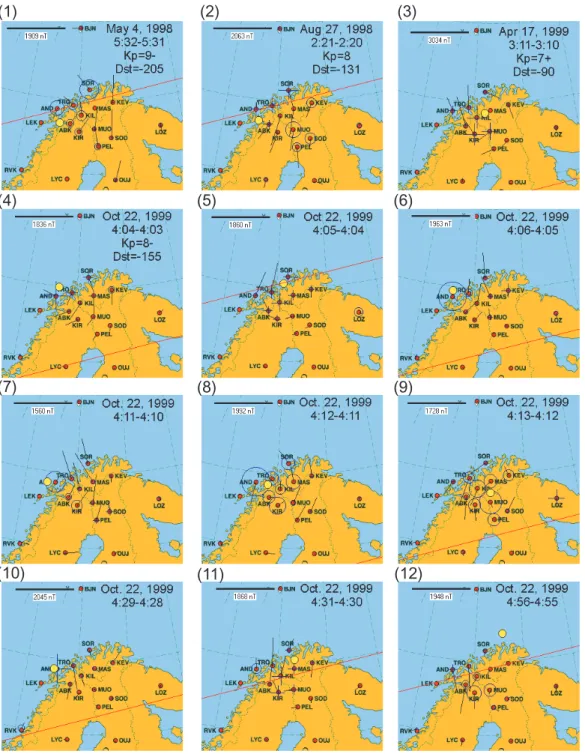
Only 10 samples with (dB/dt )max > 900 nT/min were
found in 1996–2000, their observed differential equivalent currents are presented in Fig. 3. The set of events belongs to four different magnetic storms; all the events appear in the morning MLT hours (roughly MLT = UT + 3 h for the IMAGE network). The central part of the IMAGE net-work is only shown since the disturbances at the southern-most stations are much smaller, in spite of the fact that all these examples appeared during very disturbed conditions (Kp = 7 + ...9− and Dst = −90... − 240 nT) when the
auroral oval was greatly expanded.
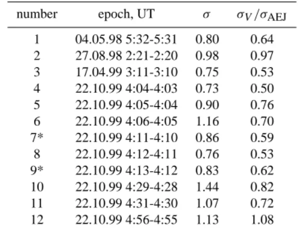
Most of the patterns shown (e.g. 1, 3, 5, 8, 11) display distinct vortex structures, and the large contribution of the vortex part is also supported by a small ratio σV/σAEJwhich
was <0.8 for 7 out of 10 samples, see Table 1.
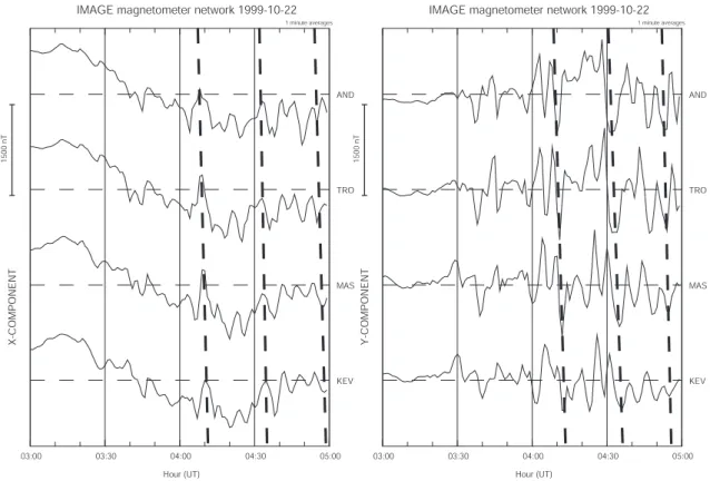
The representative magnetograms from the longitudinal chain of magnetometers are shown in Fig. 4 for the storm event which gave the most of samples in Fig. 3. The tilt of the dashed lines illustrates the eastward phase motion which is also seen in samples 4, 5 and 7, 8, 9 in Fig. 3. A no-table feature of the magnetograms is that the variations in the Y component are comparable in magnitude with those in
Table 1. The normalised standard deviation σ and the ratio
σV/σAEJfor the strongest dB/dt events.
number epoch, UT σ σV/σAEJ
1 04.05.98 5:32-5:31 0.80 0.64 2 27.08.98 2:21-2:20 0.98 0.97 3 17.04.99 3:11-3:10 0.75 0.53 4 22.10.99 4:04-4:03 0.73 0.50 5 22.10.99 4:05-4:04 0.90 0.76 6 22.10.99 4:06-4:05 1.16 0.70 7* 22.10.99 4:11-4:10 0.86 0.59 8 22.10.99 4:12-4:11 0.76 0.53 9* 22.10.99 4:13-4:12 0.83 0.62 10 22.10.99 4:29-4:28 1.44 0.82 11 22.10.99 4:31-4:30 1.07 0.72 12 22.10.99 4:56-4:55 1.13 1.08
* samples 7 and 9 were added to show the sequence of observa-tions
the X component, as typical for vortex currents. The quasi-periodicity with T ∼ 8 min, especially clear in the Y com-ponent, is visible on the magnetograms. This pulsating be-havior of the X component occurs on the background of the significant negative bay.
These examples are not exotic but are well representative for a vast majority of large dB/dt events. The strong con-tribution of the vortex part and the morning MLT occurrence will be further addressed in the following sections.
To check the relationship of these events to real GIC ef-fects, we inspected the records of geomagnetically induced currents along the Finnish natural gas pipeline at M¨ants¨al¨a (the latitude is ∼60.5 N, 30 km east of Nurmijarvi). Data have been available since November 1998, that is for 2 of our 4 storm events shown in Fig. 3. In both cases (17 April 1999 and 22 October 1999), a significant current was recorded (4 and 7 A, respectively), which is comparable to the maximal GIC (32 A, on 6 November and 24 November 2001) ever recorded at this station.
3.2 Relative contributions of 1-D and 2-D current systems After processing the data using the algorithm described in Sect. 2 we can compare the relative contributions to the stan-dard deviation from AEJ-type and vortex-type parts. The dis-tributions of σV, σAEJand total σ characterizing the relative
contributions and the fit quality were found to have shapes close to normal distributions, with mean values of about 1.2, 1.4 and 0.9 (in normalised units), respectively. To distin-guish events with dominating AEJ- or vortex-contributions we use the parameter σV/σAEJ(Eqs. 7 and 8). As a threshold
value to separate them we used 0.8 (based on their averages), i.e. samples with σV/σAEJ < 0.8 are considered as
vortex-dominated, whereas those with σV/σAEJ >0.8 are referred
to as AEJ-dominated events. Only well-recognized samples with σ < 1.0 (σ is normalised with respect to < δB >) are
S. V. Apatenkov et al.: Geometry of ionospheric current systems 67
(1)
(2)
(3)
(5)
(4)
(6)
(10)
(11)
(12)
(7)
(8)
(9)
Fig. 3. Differential equivalent current patterns for ten strongest dB/dt events in 1996-2000. One-minute differences of magnetic field values
are shown. Arrows correspond to the horizontal magnetic field vector rotated 90 degrees clockwise, circles and crosses correspond to an upward and downward vertical component, respectively. The best fit model locations of the electrojet (red line) and the vortex (yellow circle) are also shown for comparison. Vortex-dominated pattern is distinctly seen in most cases. The samples 7 and 9 were added to illustrate the dynamics.
used in this analysis, which includes about 2/3 of all events. As visual examples of the fit quality one can use Fig. 3 to-gether with Table 1.
Figure 5 (solid line) shows two main results. First, the number of vortex-dominated and AEJ-dominated events is approximately equal even at the lowest threshold values. Second, and more importantly, the contribution of
vortex-dominated samples is progressively increasing with the in-crease in the (dB/dt )max threshold. The number of
sam-ples becomes smaller with the threshold increase, so that there are only 6 well-recognized events with (dB/dt )max >
900 nT/min, but the trend of the whole plot is very reliable. By choosing other limits (thresholds) for σV/σAEJand σ we
IMAGE magnetometer network 1999-10-22 03:00 03:30 04:00 04:30 05:00 Hour (UT) X-COMPONENT 1500 nT 1 minute averages AND TRO MAS KEV
IMAGE magnetometer network 1999-10-22
03:00 03:30 04:00 04:30 05:00 Hour (UT) Y-COMPONENT 1500 nT 1 minute averages AND TRO MAS KEV
Fig. 4. Magnetograms of X and Y components from the longitudinal chain of IMAGE magnetometers (west to east, from AND to KEV)
on 22 Oct 99 displayed in Fig. 3 (samples 4–12). Some sharp features on the magnetograms are connected with the dashed line to show the eastward phase motion. Quasi-periodic magnetic variations with T ∼ 8 min were observed after 04:00 UT.
100 200 300 400 500 600 700 800 900 dB/dt threshold, nT/min 0 0.5 1 1.5 2 NAE J / N v all samples 04-08 MLT 21-01 MLT 2731/2053 6569/6017 1682/2135 29/16 125/168 63/134 9/20 6/20 1/5
Fig. 5. Ratio of the number of electrojet-dominated samples (NAEJ)
to the number of vortex-dominated samples (NV) as a function of
dB/dtthreshold. Statistics for morningside and pre-midnight sam-ples is also shown by dashed and dotted lines, respectively, the
NAEJand NV numbers are explicitly shown for some thresholds
to illustrate the statistics available.
ignore the 2-D character of the current systems when mod-eling the GIC effects, especially when we are interested in the largest events. Morningside and pre-midnight events are shown separately in Fig. 5 (dashed lines). The trend for the samples in the 04:00–08:00 MLT sector is the same, how-ever, smaller amount (see subscripts along the lines in Fig. 5)
of samples in 21:00–01:00 MLT have a larger electrojet con-tribution. As shown in the following section the number of pre-midnight samples relatively decreases for large dB/dt thresholds.
3.3 Diurnal and latitudinal variation
Viljanen et al. (2001) showed that the occurrence of large
dB/dt events displays the strong MLT variation, so we start with a study of these distributions. When doing statisti-cal analysis it is worth separating continuous series of large
dB/dt timesteps from isolated timesteps. (For example, a strong storm may produce a series of 1-min timesteps above some dB/dt threshold, at the same time this could be one event from the GIC risk point of view.) For this purpose we repeated the occurrence analysis separately for individ-ual 1-min timesteps (samples) and for the hours (i.e. it has at least one timestep exceeding the threshold).
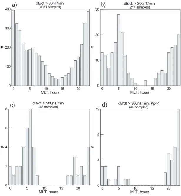
Diurnal distributions for the hours with different dB/dt thresholds are shown in Fig. 6. They all show two occurrence maxima in the pre-midnight and morning hours, respec-tively. This agrees with the results by Viljanen et al. (2001), who analysed the occurrence of events with dH /dt >1 nT/s (60 nT/min). We, however, also see interesting differences. With the lowest threshold (>30 nT/min) the picture resem-bles the pattern obtained by Viljanen et al. (2001) which has the pre-midnight maximum larger than the morning
maxi-S. V. Apatenkov et al.: Geometry of ionospheric current systems 69
a)
b)
c)
d)
0 5 10 15 20 MLT, hours 0 2 4 6 8 # dB/dt > 500nT/min (43 samples) 0 5 10 15 20 MLT, hours 0 100 200 300 400 # dB/dt > 30nT/min (4031 samples) 0 5 10 15 20 MLT, hours 0 10 20 30 # dB/dt > 300nT/min (217 samples) 0 5 10 15 20 MLT, hours 0 4 8 12 # dB/dt > 300nT/min, Kp<4 (42 samples)Fig. 6. MLT occurrence of hours which have at least one sample with dB/dt above the given threshold. The thresholds are (a) −30 nT/min, (b) -300 nT/min, (c) −500 nT/min. (d) – the same threshold as in (b), but only small Kpsamples are included.
mum. With increasing threshold the morning maximum be-comes comparable, and, then for (dB/dt)max>500 nT/min
it dominates. This is consistent with the examples of the strongest events in Fig. 3 which all occurred in the morning MLT hours.
There is an interesting exception from this trend. If we take the intermediate threshold (dB/dt)max > 300 nT/min
but isolate those events which occur under a moderate distur-bance level (Kp<4, Fig. 6d), almost all morningside events
disappear (although the total number of events decrease to
∼ 20%). This is consistent with these events (occurring in pre-midnight sector) being related to moderate substorms.
The statistics obtained separately for the hours and for
all timesteps give qualitatively similar results, although the numbers are different. Morning to pre-midnight maxima ratios for timesteps (∼1 and ∼5 for dB/dt thresholds 30 and 300 nT/min, respectively) are much larger in compari-son with those found for the hours (∼0.5 and ∼1.2, respec-tively). In other words, the main difference between the distributions for the hours (Fig. 6) and those for the sam-ples is that the morning maxima for the samsam-ples would be more pronounced. This is because the morningside events typically include the long sequences of strong variations, as seen on the magnetogram in Fig. 4. When considering the diurnal distributions separately for vortex-dominated and for electrojet-dominated samples, we obtain greater
morn-0
0.2
0.4
relative units
Kp=0..3
0.6
0.3
56
60
64
68
72
CGL
at
0
0.2
0.4
relative units
Kp=3..6
0.6
0.3
56
60
64
68
72
0
0.2
0.4
relative units
Kp=6..9
0.3
56
60
64
68
72
"vortices" "line-currents" stationsEQB
EQB
EQB
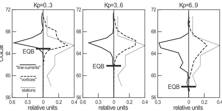
Fig. 7. Latitudinal distributions of AEJ-dominated (solid line) and vortex-dominated (dashed line) current systems. The distinction criterion
as in Sect. 3.2 is applied. The latitudinal distribution of magnetometer locations is also shown for reference (dotted line). Equatorward boundary (EQB) of the auroral oval for the morning sector at MLT 4–6 h is shown by horizontal ticks, its latitude near midnight would be
∼2◦equatorward (after Starkov, 1994).
ing maximum in the former case because vortex-dominated events predominantly occur in morning MLT hours (compare
NV and NAEJgiven in Fig. 5).
To characterize the location of the current systems in the auroral oval we also constructed the latitudinal distributions, see Fig. 7. We apply the same criterion as in Sect. 3.2 to distinguish between AEJ-dominated and vortex-dominated events. One peculiarity of Fig. 7 is that the locations of both electrojets and vortices are grouped at the latitudes which have the most dense station coverage (in the middle of net-work), and this changes very little with the increasing ac-tivity level. There could be two explanations of this effect. The first one is that those vortexes and jet currents which stay near the region of dense station coverage will be em-phasized by the method used, since these structures would give the largest contribution to the total standard deviation which is minimized by our method. This effect is inevitably present, however, we also have strong arguments in favor of natural reasons which work in the same way, at least for the strong morningside events. The observational data plotted in Fig. 3 confirm that the largest observed dB/dt are seen in the middle of observation domain, that is in the middle of the au-roral zone, many degrees poleward of the expected location of the equatorward boundary of auroral oval. Evidently, the large dB/dt vectors have comparable X and Y components, as natural for the vortex system, and these vortex structures are centered just at the latitudes where the occurrence has a peak in the Fig. 7. This has also been confirmed in the
statis-tical survey by Viljanen et al. (2001), which showed that in the morning sector the large dB/dt vectors have comparable
X and Y components at these latitudes (implying that vor-tex structures are clustered here), whereas the polarization was more electrojet-like at the southernmost stations on the morning side, or at any latitudes in the near-midnight MLT region.
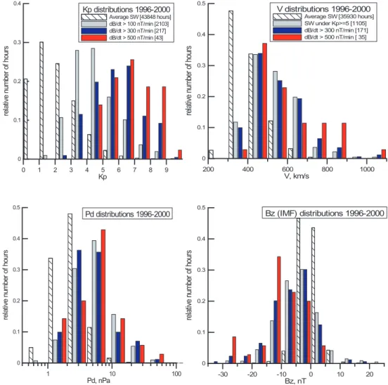
3.4 Solar wind properties during large dB/dt events With this large data base we can also address which solar wind conditions are efficient in producing the large dB/dt events. To do so, we plot the parameter distributions in the solar wind for the events above different (dB/dt )max
thresh-olds (100, 300 and 500 nT/min) and compare these distribu-tions to those characterizing the solar wind. We used hourly averaged solar wind (OMNI) data. We tested different so-lar wind parameters, but show here only those which cor-respond to the different ways in which the solar wind in-fluences the magnetosphere (dynamic pressure (P d), which controls the magnetospheric compression, and the solar wind velocity (V ) and vertical IMF component (Bz), which
deter-mine the magnetospheric electric field).
While this plot shows the expected result that strong
dB/dt events appear during disturbed times, the enhanced
V, P d and, especially, strong southward Bz are the known
conditions to result in the main phase of a magnetic storm. The plot also shows how strongly the distributions are shifted by varying the dB/dt threshold. It should be noticed that the
S. V. Apatenkov et al.: Geometry of ionospheric current systems 71 0 0.1 0.2 0.3 0.4 0.5 re la tiv e num ber of hour s Pd distributions 1996-2000 1 10 100 Pd, nPa 0 0.1 0.2 0.3 0.4 0.5 re la tiv e num ber of hour s Bz (IMF) distributions 1996-2000 -30 -20 -10 0 10 20 Bz, nT 0 0.1 0.2 0.3 0.4 re la tiv e num ber of hour s Kp distributions 1996-2000 Average SW [43848 hours] dB/dt > 100 nT/min [2103] dB/dt > 300 nT/min [217] dB/dt > 500 nT/min [43] 0 1 2 3 4 5 6 7 8 9 Kp 0 0.1 0.2 0.3 0.4 0.5 re la tiv e num ber of hour s V distributions 1996-2000 Average SW [35930 hours] SW under Kp>=5 [1105] dB/dt > 300 nT/min [171] dB/dt > 500 nT/min [ 35] 200 400 600 800 1000 V, km/s
Fig. 8. Normalized occurrence distributions of hourly averaged solar wind parameters and of Kpactivity index constructed for the average
solar wind as well as for large dB/dt events with different thresholds. Solar wind parameter distributions for Kp≥5 are also shown.
strongest events with (dB/dt)max>500 nT/min occur in the
extreme tail of the solar wind parameter distributions.
We also plot Kp distributions for different dB/dt
thresholds which show that the whole distribution shifts to larger Kp with the threshold increase, and that this
shift is much more pronounced than in any of the so-lar wind parameters (Fig. 8a). For example, events with
(dB/dt )max>300 nT/min have a maximal occurrence ratio
under Kp∼5 and never occur under Kp ≤ 2. In Fig. 8b–d
we also plotted the solar wind parameter distributions for comparison. It shows that V , P d, Bz distributions for the
events under Kp≥5 already resemble those with the
thresh-old (dB/dt)max > 300 nT/min. This fact is quite
natu-ral, since the Kp index is a measure of fluctuation range
in the magnetic field (although at larger time scales). It means that the Kp value is the best parameter which
indi-cates GICs as compared to any individual solar wind param-eter. However, only every fifth hour under Kp >5 includes (dB/dt )max>300 nT/min.
4 Discussion
Our results indicate a large contribution from vortex currents to the equivalent current systems, that produce large dB/dt and, potentially, large GIC effects. Moreover, the impor-tance of vortex currents seems to increase with an increasing
dB/dt threshold, so the strongest events are mostly due to the development of a transient current vortex. The obvious reason could be that the larger spatial gradients and/or vio-lent motions are the inherent features of 2-D structures (like the auroral bulge, WTS, omega-structures, etc.) rather than of the 1-D electrojet structure. This result is in agreement with the statistics of dB/dt events presented by Viljanen et al. (2001), whose Figs. 6 and 9 clearly indicate comparable contributions from Bxand Bycomponents which is an
inher-ent property of 2-D structures as compared to the electrojet-induced magnetic field. This occurs at the stations at 64◦–67◦ CGLat and in morning MLT hours, whereas large Byevents
were not pronounced in the pre-midnight MLT maximum (Fig. 5, dotted line). One interesting peculiarity is that
dur-ing storm conditions, this location is in the middle of the wide and expanded auroral oval at the morningside, confirm-ing the latitudinal distributions shown in Fig. 7. It may have important implications for the understanding of the magne-tospheric sources which produce strong 2-D ionospheric cur-rent structures and, therefore, large GIC effects: they are re-lated to the middle part of the magnetosphere rather than to the inner region occupied by the ring current.
Two peaks (in pre-midnight and morning MLT sectors) are observed in the diurnal distributions of large dB/dt, and they show some important differences. First, according to Viljanen et al. (2001), the polarization of the dB/dt vec-tor is mostly along the meridian in the pre-midnight events, whereas it is variable and often includes a large Y component in the morning sector. This is also in agreement with our con-clusion that AEJ and vortex structures are more important in the pre-midnight and the morning sectors, respectively. Sec-ond, the occurrence of pre-midnight events does not depend as much on the overall disturbance level (Kp) as the
morn-ingside events do (our Fig. 6d). This suggests that different sources and processes could be responsible for GIC events in these two regions.
A new feature appearing in our analysis is a strong change in the dB/dt event occurrence with the dB/dt threshold, so that the strongest events tend to appear exclusively in the morning sector in the middle of an expanded auroral oval. A number of observed characteristics allow us to identify the source of the largest dB/dt with the current system of Ps6 pulsations (e.g. Kawasaki and Rostoker, 1979) accompany-ing auroral omega bands and torch-like structures. These properties include: (1) morningside occurrence, (2) quasi-periodic magnetic variations with T ∼ 5 − 10 min, and (3) azimuthal eastward propagation. A limited number of strong
dB/dt events had good coverage by Polar UVI auroral ob-servations, and a brief inspection of these data confirm this interpretation. A more detailed investigation of auroral struc-tures associated will be presented elsewhere.
Acknowledgements. The work on the project was supported by the
INTAS project 2000-0752. S. Apatenkov and V. Sergeev thank Finnish Meteorological Institute for the support during their stays in Helsinki, their work was also supported by RFFI grant 03-05-64807 and Intergeophysics Program. We thank all institutes main-taining the IMAGE magnetometer network.
The Editor in Chief thanks J. Watermann and T. Moretto for their help in evaluating this paper.
References
Albertson, V. D. and Van Baelen, J. A.: Electric and Magnetic Fields at the Earth’s Surface Due to Auroral Currents, IEEE Trans. Power Appar. Syst., PAS-89, 578–584, 1970.
Amm, O., and Viljanen, A.: Ionospheric disturbance magnetic field continuation from the ground to the ionosphere using spherical elementary current systems, Earth, Planets and Space, 51, 431– 440, 1999.
Boteler, D. H., Boutilier, S., Bui-Van, Q., Hajagos, L., Swatek, D., Leonhard, R., Hughes, B., Ferguson, I. J., and Odwar, H. D.: Geomagnetic Hazard Assessment, Phase 2, Final Report, CEA project 357 T 848A, GSC Open File 3140, 1997.
Boteler, D. H., Pirjola, R. J., and Nevanlinna, H.: The effects of geo-magnetic disturbances on electrical systems at the earth’s surface, Adv. Space Res., 22, 17–27, 1998.
Fukushima, N.: Generalized theorem of no ground magnetic effect of vertical currents connected with Pedersen currents in the uni-form conducting ionosphere, Rep. Ionos. Space Res. Japan., 30, 35–40, 1976.
Kawasaki, K. and Rostoker, G.: Perturbation magnetic fields and current systems associated with eastward drifting auroral struc-tures, J. Geophys. Res., 84, 1464–1480, 1979.
Pulkkinen, A., Viljanen, A., Pirjola, R., and BEAR Working Group: Large geomagnetically induced currents in the Finnish high-voltage power system, Finnish Meteorological Institute, Reports, 2000:2, 99 pp., 2000.
Pulkkinen, A., Thomson, A., Clarke, E., and McKay, A.: April 2000 geomagnetic storm: ionospheric drivers of large geomagnetically induced currents, Ann. Geophysicae, 21, 709–717, 2003. Starkov G. V.: A Mathematical Description of Auroral Luminousity
Boundaries, Geomagn. Aeron., 34, 3, 80–86, 1994.
Tanskanen, E. I., Viljanen, A., Pulkkinen, T. I., Pirjola, R., H ¨Akkinen, L., Pulkkinen, A., and Amm, O.: At substorm on-set, 40% of AL comes from underground, J. Geophys. Res., 106, 13 119–13 134, 2001.
Towle, J. N., Prabhakara, F. S., and Ponder, J. Z.: Geomagnetic effects modelling for the PJM interconnection system. Part I – Earthsurface potential computaion, IEEE Trans. Power Syst., 7, 949–955, 1992.
Untiedt, J. and Baumjohann, W.: Studies of polar current systems using IMS Scandinavian Magnetometer Array, Space Sci. Rev., 63, 245–390, 1993.
Viljanen, A., Kauristie, K., and Pajunp¨a¨a, K.: On induction effects at EISCAT and IMAGE magnetometer stations, Geophys. J. Int., 121, 893–906, 1995.
Viljanen, A.: The relation between geomagnetic variations and their time derivatives and estimation of induction risks, Geophys. Res. Lett., 24, 6, 631–634, 1997.
Viljanen, A.: Relation of Geomagnetically Induced Currents and Local Geomagnetic Variations, IEEE Trans. Power Delivery, 4, 1285–1290, 1998.
Viljanen, A., Amm, O., and Pirjola, R.: Modeling Geomagneti-cally Induced Currents During Different Ionospheric Situations, J. Geophys. Res., 104, 28 059–28 072, 1999.
Viljanen, A., Nevanlinna, H., Pajunp¨a¨a, K., and Pulkkinen, A.: Time derivative of the horizontal geomagnetic field as an activity indicator, Ann. Geophysicae, 19, 1107–1118, 2001.
Viljanen, A. and Pirjola, R.: Geomagnetically induced currents in the Finnish high-voltage power system – a geophysical review, Surv. Geophys., 15, 382–408, 1994.