HAL Id: insu-01515703
https://hal-insu.archives-ouvertes.fr/insu-01515703
Submitted on 3 May 2017HAL is a multi-disciplinary open access
archive for the deposit and dissemination of sci-entific research documents, whether they are pub-lished or not. The documents may come from teaching and research institutions in France or abroad, or from public or private research centers.
L’archive ouverte pluridisciplinaire HAL, est destinée au dépôt et à la diffusion de documents scientifiques de niveau recherche, publiés ou non, émanant des établissements d’enseignement et de recherche français ou étrangers, des laboratoires publics ou privés.
Cassidy, Ronan Modolo, Jean-Yves Chaufray, R.E. Johnson
To cite this version:
François Leblanc, Apurva V. Oza, Ludivine Leclercq, Carl Schmidt, T. Cassidy, et al.. On the orbital variability of Ganymede’s atmosphere. Icarus, Elsevier, 2017, 293, pp.185-198. �10.1016/j.icarus.2017.04.025�. �insu-01515703�
ACCEPTED MANUSCRIPT
2
On the orbital variability of Ganymede’s atmosphere
F. Leblanc1, A.V. Oza1, L. Leclercq 2, 3, C. Schmidt1, T. Cassidy 4, R. Modolo.2, J.Y. Chaufray,2 and R.E. Johnson3
1
LATMOS/IPSL, UPMC Univ. Paris 06 Sorbonne Universités, UVSQ, CNRS, 4 place Jussieu 75005 Paris, France
2
LATMOS/IPSL, UVSQ Université Paris-Saclay, UPMC Univ. Paris 06, CNRS, Guyancourt, France
3
University of Virginia, Charlottesville, Virginia, USA
4
Laboratory for Atmospheric and Space Physics, University of Colorado, Boulder, CO 80303, USA
Abstract : Ganymede’s atmosphere is produced by radiative interactions with its surface, sourced by
the Sun and the Jovian plasma. The sputtered and thermally desorbed molecules are tracked in our Exospheric Global Model (EGM), a 3-D parallelized collisional model. This program was developed to reconstruct the formation of the upper atmosphere/exosphere of planetary bodies interacting with solar photon flux and magnetospheric and/or the solar wind plasmas. Here, we describe the spatial distribution of the H2O and O2 components of Ganymede's atmosphere, and their temporal
variability along Ganymede’s rotation around Jupiter. In particular, we show that Ganymede's O2 atmosphere is characterized by time scales of the order of Ganymede's rotational period with Jupiter's gravity being a significant driver of the spatial distribution of the heaviest exospheric components. Both the sourcing and the Jovian gravity are needed to explain some of the
characteristics of the observed aurora emissions. As an example, the O2 exosphere should peak at the equator with systematic maximum at the dusk equator terminator. The sputtering rate of the
ACCEPTED MANUSCRIPT
3
H2O exosphere should be maximum on the leading hemisphere because of the shape of the open/close field lines boundary and displays some significant variability with longitude.
I Introduction
Ganymede is the only known satellite with an intrinsic magnetosphere (Kivelson et al. 1996). Its icy surface is eroded by the solar radiation flux and by the Jovian energetic plasma leading to a locally-collisional atmosphere and a locally surface-bounded exosphere (Stern 1999; Marconi 2007; Turc et al. 2014; Plainaki et al. 2015; Shematovich 2016). Unfortunately, Ganymede's atmosphere remains essentially unknown despite the flybys during the mission Galileo in the 90s. This mission detected only one atmospheric emission, Lyman α, interpreted as being produced by resonant scattering by exospheric atomic hydrogen (Barth et al. 1997) with a column density around 9.211012 H/cm2. Such a column density and its variation with distance to Ganymede suggested a surface density around 1.5104 H/cm3 and an exospheric temperature around 450 K. Hubble Space Telescope was also able to identify another component of Ganymede atmosphere, the O2 molecule through the observations of two UV atomic oxygen emissions with intensities corresponding to a column density around 1 to 101014 O2/cm2 (Hall et al. 1998). Since this discovery, several other HST observations of these emission have revealed their auroral origin (Feldman et al. 2000; McGrath et al. 2013; Saur et al. 2015) highlighting the relations between the spatial distribution of these emissions, Ganymede's intrinsic magnetospheric structure (Kivelson et al. 1996) and Ganymede's surface's albedo (Khurana et al. 2007).
Gurnett et al. (1996) published the first observations of Ganymede's ionosphere by the plasma wave spectrometer (PWS) on board Galileo suggesting ion densities on the order of 100 cm-3 and a scale height around 1000 km. This first set of measurements was later complemented by a second flyby (Eviatar et al. 2001b) confirming the density range but suggesting that a number density on the order of 1000 cm-3 at the surface may be more realistic and in better agreement with the upper limit set by
ACCEPTED MANUSCRIPT
4
radio occultation (Kliore 1998). Measurements by the Plasma Science (PLS) instruments were also performed during Galileo flybys in the polar regions of Ganymede (Frank et al. 1997). These authors reported the observations of hydrogen ions outflowing from Ganymede's poles with temperatures around 4×10⁴ K and surface densities around 100 cm-3. These observations were later reanalyzed by Vasyliunas and Eviatar (2000) suggesting that O ions rather than H ions constitute this outflow, with similar densities as derived by Frank et al. (1997). These sets of observations of the thermal ionosphere were complemented by energetic ion measurements obtained by EPD/Galileo, showing that Ganymede is permanently embedded in an energetic plasma mainly composed of S+ and On+ (Paranicas et al. 1999).
After Galileo flybys, a simple 1-D model of the atmosphere and ionosphere was proposed by Eviatar et al. (2001a) to fit PWS profiles with O2 densities at the poles around 106 cm-3. The first attempt to reconstruct the origins and fate of Ganymede’s neutral environment was described in Marconi (2007) who developed a 2-D axi-symmetric model of this atmosphere using a combination of Direct Simulated Monte Carlo and Test-particle Monte Carlo simulations focusing on the sunlit trailing hemisphere. He suggested neutral densities peaking around 109 cm-3 around the subsolar region and 108 cm-3 at the poles with the two main atmospheric species being H2O and O2. Turc et al. (2014) developed the first 3-D model of Ganymede’s atmosphere starting from Marconi (2007) simulation for the sunlit trailing hemisphere. These authors found essentially the same surface density but some discrepancies were found at high altitudes. Turc et al. (2014) found a Lyman α emission brightness up to 70 times smaller than observed by Barth et al. (1997), whereas Marconi (2007) had to multiply his simulated H Lyman α by a factor 4 to reproduce the observed intensities. Both models were able to reproduce the O2 emission intensity observed by HST (Hall et al. 1998; Feldman et al. 2000). Furthermore, Plainaki et al. (2015) developed a 3-D Monte Carlo model of Ganymede's exosphere, including a model of ion precipitation in the auroral regions using a global MHD model of Ganymede's magnetosphere (Jia et al. 2009). They modeled Ganymede's sunlit leading hemisphere highlighting the different exospheric regions of the two main components H2O and O2.
ACCEPTED MANUSCRIPT
5
In this paper, we improve Turc et al. (2014) model, implementing a collisional scheme in order to identify the changes induced by atmospheric particle collisions. Marconi (2007) nicely illustrated the remarkable nature of this exosphere/atmosphere by plotting his estimate of the Knudsen number around Ganymede. Ganymede’s atmosphere is predicted to be locally collisional (around the subsolar region) and collisionless elsewhere. Another aspect of Ganymede that was not described in Marconi (2007) or Turc et al. (2014), is how this atmosphere might change along Ganymede’s orbit due to both its rotation and Jupiter's gravitational field. These new simulations take into account the revolution of Ganymede around Jupiter and Jupiter’s gravitational field. In Section II, we present the main improvements of our model with respect to Turc et al. (2014). Section III presents how this work could contribute to a better understanding of Ganymede's atmospheric formation and evolution and is followed by a brief comparison with the few observations of this atmosphere and with other similar observations in our solar system in section VI.
II Exospheric Global Model
II.1 Application to Ganymede
A first version of the Exospheric Global Model (EGM) was applied to the description of Ganymede's atmosphere in Turc et al. (2014). This is a 3-D Monte Carlo model describing the fate of test-particles, ejected from a surface or an atmosphere of a planet or satellite, and subsequently followed under the effect of gravitational fields until their escape (when reaching an upper limit set at few planetary radii from the surface), their ionization/dissociation (by photo and/or electron impacts), or until their readsorption at the surface (which is species dependent). In order to reconstruct density, velocity, and temperature of the exospheric species (minor and major components), this model was parallelized inducing a very significant reduction of the restitution time and the possibility to use much larger total memory. These two improvements were crucial to describe the spatial and temporal distributions of all exospheric species in synchrony, that is, in the case of Ganymede's icy
ACCEPTED MANUSCRIPT
6
surface, all H2O products, namely H2O, H2, H, O2, O and OH. The list of the reactions taken into account in our model is given in Table 2 of Turc et al. (2014) and is reproduced in Table 1 below.
Reactions Rate (s-1) Excess Energy (eV) References
H + hν H+ + e 4.5×10⁻⁹ 3.8 Huebner et al. (1992) H2 + hν H + H 8.8×10⁻⁹ 2.2 Marconi (2007) H2 + hν H2+ + e 3.1×10⁻⁹ 6.9 Huebner et al. (1992) H2 + hν H+ + H + e 6.9×10⁻¹⁰ 26 Huebner et al. (1992) O + hν O+ + e 1.5×10⁻⁸ 24 Huebner et al. (1992) OH + hν O + H 9.7×10⁻⁷ 3.4 Marconi (2007) OH + hν OH+ + e 1.6×10⁻⁸ 22 Huebner et al. (1992) H2O + hν H + OH 5.2×10⁻⁷ 3.4 Marconi (2007) H2O + hν H2 + O 3.8×10⁻⁸ 3.4 Marconi (2007) H2O + hν H + H + O 4.9×10⁻⁸ 4.6 Marconi (2007)
H2O + hν H + OH+ + e 3.8×10⁻⁹ 21 Huebner et al. (1992) H2O + hν H2 + O+ + e 5.2×10⁻¹⁰ 38 Huebner et al. (1992) H2O + hν OH + H+ + e 1.0×10⁻⁹ 28 Huebner et al. (1992) H2O + hν H2O+ + e 2.1×10⁻⁸ 14 Huebner et al. (1992)
O2 + hν O + O 2.0×10⁻⁷ 1.3 Marconi (2007)
O2 + hν O2+ + e 3.0×10⁻⁸ 18 Huebner et al. (1992) O2 + hν O + O+ + e 8.4×10⁻⁹ 26 Huebner et al. (1992)
Reactions Rate (cm3 s-1) Excess Energy (eV) References
H + e H+ + e + e 9.1×10⁻⁸ 3.8 Ip (1997) H2 + e H + H + e 9.6×10⁻⁹ 4.6 Marconi (2007) H2 + e H2+ + e 1.6×10⁻⁸ 6.9 Ip (1997) H2 + e H+ + H + e + e 9.6×10⁻¹⁰ 26 Ip (1997) O + e O+ + e + e 2.0×10⁻⁸ 24 Ip (1997) OH + e O + H 1.2×10⁻⁸ 3.4 Ip (1997) OH + e OH+ + e + e 2.8×10⁻⁸ 22 Ip (1997) H2O + e OH + H + e 3.7×10⁻⁸ 3.4 Marconi (2007) H2O + e H2 + O + e 1.6×10⁻⁸ 3.4 Ip (1997)
H2O + e OH + H+ + e + e 4.3×10⁻⁹ 28 Smyth and Marconi (2006)
H2O + e H + OH+ + e + e 4.0×10⁻⁹ 21 Ip (1997)
H2O + e H2 + O+ + e + e 7.1×10⁻⁹ 38 Ip (1997)
H2O + e H2O+ + e + e 2.1×10⁻⁸ 14 Ip (1997)
O2 + e O + O + e 1.3×10⁻⁸ 1.3 Marconi (2007)
O2 + e O2+ + e + e 2.0×10⁻⁸ 18 Ip (1997)
O2 + e O + O+ + e + e 1.1×10⁻⁸ 26 Smyth and Marconi (2006)
Table 1: Photon and electron ionization and dissociation in Ganymede's atmosphere (Turc et al.
ACCEPTED MANUSCRIPT
7
When impacting the surface, test-particles can either stick or be re-ejected at once. As in Turc et al. (2014) and Marconi (2007), electron ionization and dissociation impacts are described considering a uniform mono-energetic electron in the Alfven wings of Ganymede’s magnetosphere (open field line regions, see section II.4) with an electron number density of 70 cm-3 and average energy of 20 eV. In the closed field lines region, we neglected ionization and dissociation by electron impacts. We assume that O2 and H2 species never stick to the surface, whereas all other species have a non-zero reabsorption probability.
Jupiter’s gravitational force at the surface of Ganymede is equivalent to a few percent of Ganymede’s gravitational force. However, because certain species have very long lifetimes in Ganymede's exosphere (e.g. H2 and O2), Jupiter’s gravity may play a significant role in shaping its exosphere, as will be shown in Section III. Because we track molecules in Ganymede’s reference frame, the Coriolis and centrifugal forces act on Ganymede’s molecules in its atmosphere throughout the orbit. This is only relevant for certain species as the rotation period is 7.2 days.
In Ganymede's inertial frame, the subsolar point rotates continuously, so that the day-to-night surface temperature gradient drives a global migration of the exospheric species towards the nightside. On the nightside, these particles can be readsorbed on the surface or thermally accommodate and be immediately re-emitted generating a peak in atmospheric density near the surface, as observed on the Moon (Hodges et al. 1974). We also introduce the possibility that returning volatiles can permeate the regolith or be transiently adsorbed. These can eventually return to the exosphere, a process potentially important for minor exospheric species, like Na, at Europa (Leblanc et al. 2005).
The standard outputs from this simulation are the 3-D values of the density, velocity, and temperature of all species considered. We therefore define a 3-D grid with 100 cells in altitude distributed exponentially from a cell of width 3 km in altitude at the surface to 300 km cell at 3 Ganymede radii (RG), with 40 cells linearly spaced in longitude, and 20 cells in latitude, defined such
ACCEPTED MANUSCRIPT
8
that all cells have the same volume at a given altitude. We also reconstructed 2-D column density maps as derived from the 3-D neutral density, 2-D emission rates for the three main emission features observed around Ganymede (Lyman α and 130.4 and 135.6 nm oxygen) and a 2-D map of the surface reservoir. The model also calculates 3-D ionization rates by electron and photon impacts.
In the following, we describe the main improvements in the model of Turc et al. (2014), namely, a new thermal surface temperature model of the surface (Section II.2), a new description of sublimation (Section II.3), a new description of sputtering (Section II.4), the introduction of collisions (Section II.5) and a fusion scheme for the test-particles (Section II.6).
II.2 Surface temperature
Ganymede's surface temperature is estimated using a one-dimensional heat conduction model in which the thermal properties of the ice are treated as two layers (Spencer et al. 1989; available via http://www.boulder.swri.edu/ spencer/thermprojrs). A low thermal inertia, 2.2×10⁴ erg cm-2 s-1 K-0.5, is assumed in the first few cm where the ice is heavily weathered, while the ice at depth has a much larger thermal inertia of 7×10⁴ erg cm-2 s-1 K-0.5, resulting in a longer thermal time scale. Density is set to 0.15 and 0.92 g/cm3 in the top and bottom layers, respectively. The albedo is assumed to vary linearly over the body's longitude, from 0.43 on the leading hemisphere to 0.37 on the trailing (Spencer, 1987), and the emissivity is set at 0.96. A small correction for the latent heat of sublimation is included (Abramov and Spencer, 2008). Solar insolation over a synodic day is determined in degree increments of longitude with an eclipse length near equinox. This approach provides a basic
description of longitudinal asymmetries about the subsolar axis that result from the thermal inertia of the ice, but does not account for any local variation of thermophysical parameters. Figure 1a shows the subsolar temperature as a function of orbital longitude, which results from shadowed sunlight during eclipse and albedo. Figure 1b maps the surface temperature at 270° orbital longitude (trailing) where a temperature of 146° K is the diurnal maximum.
ACCEPTED MANUSCRIPT
9
Figure 1: a: Evolution of the subsolar surface temperature with respect to Ganymede orbital longitude (or phase angle). The insert in panel a is a zoom on the eclipse period showing the typical length of the eclipse and its impact on the subsolar surface temperature. b: Map of the surface temperature at 270° Ganymede phase angle with respect to latitude and West longitude. The subsolar point is at a latitude of 0° and a west longitude of 270° (white cross). Dawn and Dusk terminators are represented by the vertical dashed lines and labeled accordingly.
As shown in Figure 1, the subsolar surface temperature peaks when Ganymede's trailing hemisphere is illuminated and is minimum at leading because of the change in surface albedo. The surface temperature displays a small but clear shift towards the afternoon due to lag from thermal inertia. The afternoon side (between 270° to 0° west longitude) of the surface is therefore significantly hotter than the morning side (between 180° and 270° west longitude).
II.3 Sublimation
In Marconi (2007), the sublimation rate at Ganymede's surface at a given temperature was given by
F = a × Ts-0.5 × exp(-b/Ts) [cm-2 s-1] (2)
with a=1.1×1031 cm-2 s-1 K1/2 and b = 5737 K. Fitting the calculation by Johnson et al. (1981), we found different values for a = 1.92×1032 cm-2 s-1 K1/2 and b = 6146 K. Fray and Schmitt (2009) published
ACCEPTED MANUSCRIPT
10
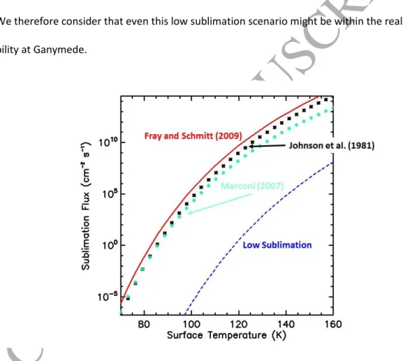
another formulation for this sublimation rate, also used by Vorburger et al. (2015). We fit the method of Vorburger et al. (2015) with equation (2) and derived values for a=2.17×1032 cm-2 s-1 K1/2 and b = 5950 K (section II.2). These three sublimation rates are shown in Figure 2 below. We also considered a case where sublimation rate was significantly decreased (low sublimation case in Figure 2) to simulate an H2O exosphere dominated by sputtering. The Fray and Schmitt (2009) sublimation model represents an ideal case, based on experiments for pure crystalline ice. In practice,
sublimation is highly dependent on the local grain structure and on an exact knowledge of the surface temperature, an error of 10 K giving a few orders of magnitude difference in sublimation rate. We therefore consider that even this low sublimation scenario might be within the realm of plausibility at Ganymede.
Figure 2: Sublimation rate with respect to surface temperature as suggested by Fray and Schmitt (2009), red solid line, by Johnson et al. (1981), cross black symbols and by Marconi (2007) in square green symbols. The dashed blue line is the rate used for the low sublimation case throughout this paper.
ACCEPTED MANUSCRIPT
11
In the results presented below, we will use the Low sublimation case (Sections III, III.1 and III.2) to model the sublimation as well as Fray and Schmitt (2009) sublimation scenario (in Section III.3) to illustrate how a strong sublimation rate could change the structure and content of the exosphere.
II.4 Sputtering
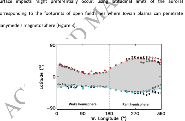
Sputtering is due to energetic Sn+ and On+ Jovian particles that penetrate Ganymede’s intrinsic magnetosphere through the polar regions and impact the polar surface regions (Cooper et al. 2001). This bombardment leads to the ejection of surface species, in particular H2O, O, H, and OH, but also the production of O2 and H2 by radiolysis in the regolith in which the molecules leave with near thermal speeds. In order to describe the spatial distribution of this bombardment, in Turc et al. (2014), we arbitrarily limited the sputtering to latitudes above 45° as did Marconi (2007). However, based on the McGrath et al. (2013) auroral observations, we map out more precise regions where surface impacts might preferentially occur, using latitudinal limits of the auroral regions corresponding to the footprints of open field lines where Jovian plasma can penetrate through Ganymede's magnetosphere (Figure 3).
Figure 3: Position of the peak auroral emission brightness as reported by McGrath et al. (2013) in a west longitude - latitude map (black symbols). The red and blue symbols represent the polynomial fit performed in our model to reproduce the closed/open field line boundaries in each hemisphere. The
ACCEPTED MANUSCRIPT
12
magnetosphere is most compressed in the ram direction at a longitude of 270°, corresponding to a higher latitude boundary. The grey region corresponds closed Ganymede field lines where we assume negligible sputtering.
By excluding the closed field line regions, we neglect any surface production of exospheric particles by sputtering here, because according to Fatemi et al. (2016) and Leclercq et al. (2016), the total precipitation rate in the closed field line region is much smaller than the total precipitation rate in the opened field line region (see also Plainaki et al. 2015). However, ions reaching the closed field line region are more energetic and should, on average, correspond to particles that sputter with higher yield, an issue that has not been addressed in Fatemi et al. (2016) and Leclercq et al. (2016). In the following, we neglect this contribution for simplicity. In the open field line regions, we assume a uniform incident ion flux on the surface as suggested by Fatemi et al. (2016) and Leclercq et al. (2016). No variation of the precipitating flux with respect to Jupiter plasma centrifugal equator or sheet has been included in this modelling for simplicity.
To calculate the efficiency of an impacting ion to sputter surface particles, we include the surface temperature dependence of the yield by Cassidy et al. (2013). Following their approach, we used Johnson et al. (2009) and Fama et al. (2008) approximations of the yield (number of molecules and atoms ejected per impacting particle) with respect to the incident energy:
YH2O(T) = YH2O(T0)× (1 + 220×exp(-0.06 eV/kB T) (3)
and
YO2(T) = YO2(T0) × (1 + 1000×exp(-0.06 eV/kB T) (4)
for sputtered H2O molecules (equation (3)) and O2 molecules (equation (4)). From these two equations, and knowing the expected flux of ion impacting the surface, we calculate the sputtered
ACCEPTED MANUSCRIPT
13
flux from Ganymede’s icy surface. However, the value of YO2(T0) for O2 and YH2O(T0) for H2O needs to be estimated as it depends on many parameters, such as the energy and charge of the impacting particle, the surface structure, and the non-ice components (Teolis et al. 2016). Another approach is to choose Y(T0) in order to reproduce the observed quantities in Ganymede's exosphere. For instance, the observed FUV O2 auroral emission can be directly used to constrain Y(T0) (see also the discussion in Section IV). Based on such observations, we can infer an effective yield of O2 molecules and then derive corresponding effective yields for the other water products H, O, OH, H2, and H2O from their known relative yields with respect to O2.
Marconi (2007) considered relative yield values equal to 1 for H2O, 1/18 for H, O, OH, to 16 for H2 and to 8 for O2, whereas Smyth and Marconi (2006) suggested values equal to 1 for H2O, 1/17 for H, O, OH, to 2 for H2 and to 1 for O2 at Europa. At Europa, Shematovich et al. (2005) considered that 1 molecule of H2O should be ejected for each 1/10 O2 molecules. Noting the wide range in previous models, we choose to base our yields on Cassidy et al. (2013), who made the first detailed calculation of sputtering rates at Europa based on laboratory experiments, Europa's expected surface temperature, and the expected intensity and spatial distribution of the impacting ions flux. These authors estimated that 2×1027 H2O/s and 1026 O2/s should be ejected from Europa's surface. In a companion paper, we applied the EGM model to Europa's atmosphere (Oza et al. 2016) and thereby constrained Y(T0) for O2 and H2O from the Cassidy et al. (2013) calculations of the total rates ejected from Europa's surface. According to Oza et al. (2016), each time a molecule of H2O is ejected from the surface, an average of 1/20 O2 is ejected from Europa's surface. The relative yield for H2 should be nearly stoichiometric, i.e. twice that of O2, since they dominate the product composition and are both formed by radiolysis of the icy surface. H, O, and OH yields should be small with respect to O2, H2 and H2O yield and are set to 1/20th of the O2 yield in agreement with Smyth and Marconi (2006). These yields represent a weighted average over all charge states of O and S ions sourced in Io's plasma torus, which bears little compositional differences between 9.4 and 15 Jovian radii (Delamere et al., 2005).
ACCEPTED MANUSCRIPT
14
When an exospheric particle is ejected from the surface by sputtering, we proceed in the same way as in Turc et al. (2014). Namely, H2O, O, H, and OH are ejected from the surface following an energy distribution described in equation (8) in Turc et al. (2014) and following a Maxwell-Boltzmann distribution at the local surface temperature in the case of O2 and H2 (equation 7 in Turc et al. 2014). In order to properly describe the entire energy distribution up to the escape energy, we bin these two energy distributions into 15-to-25 energy intervals (from 0 to an energy slightly above the escape energy) and simultaneously eject 15 to 25 individual test-particles with a weight calculated as the integral of the energy distribution over the energy range of each bin. Teolis et al. (2016) suggested that O2 molecules could be ejected following the sum of two distributions: 70% of the O2 being ejected following a Maxwellian Boltzmann distribution and 30% being ejected following a distribution in E/(U+E)3 (Johnson et al. 1983). Such a choice would populate the higher altitudes slightly more efficiently than in our approach but would not change the main conclusions of this paper.
II.5 Collisional scheme
Because in some regions of Ganymede’s atmosphere, collisions between atmospheric particles might shape the density (Marconi 2007), we also include collisions between molecules and atoms. At each time step, the total density of each species in a cell is calculated. From these densities, the maximum number of collision pairs between each test-particle and the other test-particles for a given species in the cell is calculated using the approach described in Bird (1994) with cross sections taken from Lewkow and Kharchenko (2014). These authors developed a new scheme including cross sections depending on both energy and angle that allows an accurate description of collision between any species colliding with energies below a few tens of eV. Typical collision cross sections for molecule-molecule or molecule-molecule-atom collision at 1 eV are 4.8×10⁻¹⁵ cm-2 and do not depend neither significantly on energy between 0 to few eVs nor on the species considered in this work (H, H2, O,
ACCEPTED MANUSCRIPT
15
equal to 6.9×10⁻¹⁵ cm-2 for H2O-H2O collision or to 3.9×10⁻¹⁵ cm-2 for O2-O2 collision. We then randomly select a number of test-particle pairs equal to the expected maximum number of collisions that should occur according to Bird (1994). One of the difficulties when including minor species is that test-particles, in a given cell, might have very different weights (i.e. they might represent vastly different number of real particles). We therefore developed a new scheme to treat such collisions. For a test-particle A of weight WA and species SA, we randomly determine with which species, SB, a test-particle A will most likely collide. We then randomly select nA test-particles Bi of weight WBi of the species SB in order to have ∑ ≥ WA. For each pair of test-particles Bi and A, we then evaluate the likehood of a collision taking into account the relative velocity between A and Bi. If a collision occurs, we determine new velocity vector after the collision, V'Ai and V'Bi following Lewkov and Kharchenko (2014). We then create a new test-particle Ai with velocity V'Ai and weight and repeat that scheme nA times. The weight of the particle A is then reduced by WBi. The velocity of each Bi test-particle after collision is equal to V'Bi with the exception of the nAth Bi test-particle which is divided into two particles: one with velocity V'BnA and weight W'BnA = WA - ∑ and the other with velocity VBnA and weight WBnA - W'BnA.
All collisions occur with energies below 10 eV so that molecular dissociation is negligible.
II.6 Fusion scheme
Since the collisional scheme implies the creation of new particles (see section II.5), we also had to implement a fusion scheme in order to limit the number of test-particles followed by the model at a given time. We tested two approaches to merge test-particles, both suggested by Lapenta (2002), the binary scheme, and the tertiary scheme. The binary scheme is faster and since it leads to similar results, we employ it. The binary scheme consists in selecting a pair of test-particles A and B which are close each other in phase space (with positions qA and qB, velocities VA, VB and weight WA, WB respectively) of the same species and in the same cell that minimizes (WA + WB)(VA² - VB²). We then
ACCEPTED MANUSCRIPT
16
create a new particle with weight equal to W=WA+WB, position equal to q = (WAqA + WBqB)/(WA+WB) and velocity equal to V = (WAVA + WBVB) / W.
For every arbitrarily fixed number of time steps (typically one hundred time steps), we count the number of particles of each species within one cell. If this number is larger than a threshold, defined as to avoid too many test-particles of a given species in a cell, the fusion scheme is activated, adapting to the computational load this presents. Test-particles are therefore selected following the approach described above, and are merged as long as this number continues to exceed the threshold.
III Ganymede’s atmosphere
In the following, we will use the phase angle of Ganymede (equivalent to its sub-observer longitude) to indicate its position around Jupiter. A phase angle of 0° corresponds to Ganymede being in the shadow of Jupiter at midnight local time (eclipse), whereas phase angles of 90° and 270° correspond to the sunlit leading hemisphere apex and sunlit trailing hemisphere apex respectively. Positions at the surface are defined using west longitude (increasing with local time), 0° planetary longitude being the subsolar point at a 0° phase angle. The simulation is performed in a GphiO rotating frame with the x-axis always pointing along the corotational direction, y-axis pointing towards Jupiter, and the z-axis pointing towards Ganymede's north pole (the x and y z-axis are inside the orbital plane of
Ganymede). Section III.1 is dedicated to the description of the fate of Ganymede's exosphere along its rotation around Jupiter, without taking into account the effect of collision between atmospheric particles, an issue specifically discussed in Section III.2. Section III.3 is based on simulations where collisions were also neglected.
Using the sputtering description in section II.4, the typical surface temperatures of Figure 1, and the low sublimation rate as described in Figure 2, the global sublimated flux is equal to 8.0×10²¹ H2O/s whereas the average ejected flux by sputtering is equal to 8.0×1027 H2O/s, 3.6×1026 O2/s, 7.2×1026 H2/s and 1.0×1025 H, O and OH/s. Marconi (2007) and Turc et al. (2014) used a flux of 1.5×1026 H2O/s
ACCEPTED MANUSCRIPT
17
and 1.2×1027 O2/s for sputtering, whereas Plainaki et al. (2015) used a flux of 7×1025 H2O/s for sputtering and 7×1029 H2O/s for sublimation using the same model for sublimation as in Marconi (2007) and Turc et al. (2014) (green square symbols in Figure 2).
We simulated more than 4.5 rotations of Ganymede around Jupiter in two weeks on 64 CPUs (that is, 3.7×10⁶ time steps of 0.75 s each for a total of 780 simulated hours). During that run, 2.6×10⁷ H2O test-particles (simulating a total of 2.2×1034 H2O molecules) and 2.1×10⁷ O2 test-particles (for 1034 O2 molecules) were ejected from the surface. Of these 1.2×10⁶ H2O test-particles escaped the simulation domain, 2.4×10⁷ were reabsorbed in the surface, 6×10⁵ were dissociated or ionized and none were merged (meaning that the maximum number of test-particles in a cell allowed by the simulation was never reached for H2O). For O2, 1.3×10⁶ were dissociated or ionized, 1.9×10⁷ were merged. The 3×10⁵ O2 test-particles which escaped the simulation domain were generated from the tail of the energy distribution ejected from the surface. Being associated with very small weight, these escaping molecules represented an escaping flux of 6×10¹⁷ O2/s. Merging test-particles is much more
important for O2 than for H2O, because O2 test-particles are essentially confined near the surface. At each time, a total number of 1 to 2×10⁶ test-particles are followed. After convergence towards a steady state, the typical escape rates are 1.6×1027 H2O/s, 6×10¹⁷ O2/s, 1.7×1026 O/s, 1.2×1026 OH/s, 3.0×1026 H2/s and 2.3×1026 H/s.
III.1 Seasonal variation of Ganymede’s exosphere
A main improvement with respect to previously published models of Ganymede's atmosphere is that we describe the evolution of Ganymede's exosphere throughout Ganymede's orbit around Jupiter while taking into account the influence of Jupiter’s gravitational field. By simulating a period of time long enough to cover several Ganymede orbits, our model simultaneously calculates the motions of all individual test-particles in Ganymede's inertial frame as well as the motion of Ganymede around Jupiter. In general, only three orbits are needed to achieve a steady state exosphere on Ganymede.
ACCEPTED MANUSCRIPT
18
Steady state is evaluated at a fixed phase between two successive orbits for a given time t, when the reconstructed density, velocity, and temperature of the O2 and H2O exospheric components and their loss rates vary by less than a few percent. In the results presented in this section, collisions are not taken into account for the following results and will be specifically discussed in section III.2.
Most previous models have focused on one specific position of Ganymede corresponding to fixed solar illumination and ram directions: the trailing illuminated hemisphere case in Turc et al. (2014) and Marconi (2007), and the leading illuminated hemisphere case in Plainaki et al. (2015). However, Ganymede's rotation implies that the geographical regions where sputtering and sublimation rates reach a maximum, rotate with respect to one another. One direct consequence of this rotation is a variable sputtering efficiency since yields depend strongly on the surface temperature and,
therefore, on the solar zenith angle (Cassidy et al. 2013).
The typical time for O2, ejected at the equator to migrate from one hemisphere to the other (that is to move from a position at the surface to its opposite position on the other side of the satellite) can be roughly estimated following Hunten et al. (1988). According to these authors, the collisionless migration time of a particle moving in a surface-bounded exosphere is on the order of tm= tb² where tb = 2(H/g)1/2 is the ballistic hop time and =RG/H. RG is Ganymede's radius and H is the scale height H=kBTS/ (mg) with kB the Boltzmann constant, TS the surface temperature (as defined in section II.2), m the mass of the particle and g the gravitational acceleration at the surface. For an O2 ejected from noon at the sunlit trailing hemisphere to migrate across the hemisphere is, tm765 hours or more than 4 orbital periods using Ts=143.5 K (see Figure 1a), H = 26 km, =101, tb=270 s. Migration across the hemisphere takes tm1690 hours, or more than 9 orbits using 85K, H=15 km, =171, tb=208 s. Precise migration times are not very meaningful, since tm well exceeds the diurnal timescale of the thermal wave, yet, the calculation is useful to conceptualize the atmosphere's diffusion. Given that the typical lifetime of an O2 is on the order of one orbital period, newly ejected O2 roughly fixed in Ganymede’s reference frame moves therefore in local time due to Ganymede's rotation. The typical
ACCEPTED MANUSCRIPT
19
time scale for the formation of the O2 exosphere can be estimated by dividing the average vertical column density (2.4×10¹⁴ O2/cm2) by the average ejection rate (3.5×10⁸ O2/cm2/s) or 190 hours, that is, more than one orbital period. Therefore, the O2 exosphere at a given orbital position will depend on its history and evolution over about one Ganymede revolution. Because the H2O molecules are quickly reabsorbed in the surface, the timescale of the H2O exosphere is much shorter than one rotational period. In the case of H2, due to its low mass, the H2 exospheric will rapidly form across Ganymede becoming spatially uniform on timescales much shorter than an orbital period and is, therefore, less dependent on localized production.
ACCEPTED MANUSCRIPT
20
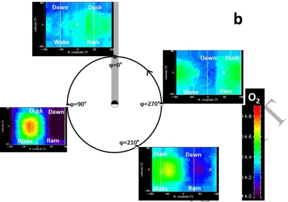
Figure 4: Vertical column densities (log10 cm-2) of the H2O (panel a) and O2 exospheres (panel b) at
different Ganymede phase angles (90°, 210°, 270° and 0°) with respect to latitude (vertical axis) and west longitude (horizontal axis) in the low-sublimation scenario. The subsolar point is indicated by the black or white cross on each panel, the dusk and dawn terminators by vertical dashed black or white lines. The ram and wake hemispheric centers are also indicated. Ganymede’s direction of rotation is indicated by the counter-clockwise arrow in the plane of Jovian co-rotation. Jupiter is at the center of each figure.
In Figure 4, we display the vertical column densities of H2O (panel a) and O2 (panel b) at four positions around Ganymede. Each figure corresponds to the average simulated density over a 6° interval centered on the indicated phase angle value. This interval allows the simulation to reach a reasonable signal-to-noise ratio for the reconstructed densities. The H2O vertical column density peaks most of the time (except at 270° phase angle) on the plasma-wake hemisphere (also the leading hemisphere) because H2O is predominantly produced by sputtering. In the low sublimation rate scenario displayed here, sputtering should occur at lower latitudes on the wake hemisphere
ACCEPTED MANUSCRIPT
21
than on the ram hemisphere (as suggested by the opened/closed field lines boundary in Figure 3), more H2O is therefore ejected on the wake hemisphere than on the ram hemisphere. This
magnetospheric effect, when convolved with the strong thermal dependence of radiolysis (Equation 3) and sublimation (Figure 2), effectively increases the H2O ejection rate at the sunlit leading
hemisphere/plasma wake (see also Plainaki et al. 2015). We therefore simulate a slightly denser H2O exosphere on the leading illuminated hemisphere position (radial column density of 1.5×10¹³
H2O/cm2) than on the trailing illuminated hemisphere position (radial column density of 1.3×10¹³ H2O/cm2). Observed from the Earth, the average line-of-sight (LOS) column density at a phase angle of 90° over the hemisphere disk would be equal to 3.4×10¹³ H2O/cm2, whereas it would decrease to 2.9×10¹³ H2O/cm2 at a phase angle of 270° (see also Figure 6). H2O in the equatorial plane has
densities smaller than 105 H2O/cm3 coming essentially from the polar region, whereas densities at the poles, are greater by two orders of magnitude. Since H2O molecules efficiently stick to the surface, the polar H2O molecules do not migrate efficiently towards the equatorial regions and remain confined around their ejection region.
The O2 exosphere is significantly different at the equatorial regions because the probability for O2 to stick to the surface, even at coldest nightside surface temperatures, is low. Consequently, the O2 exosphere is spread across all longitudes and latitudes. There is however a clear dusk/dawn asymmetry of the O2 spatial distribution with a peak in density at afternoon between =90° to
=200°, Ganymede local time and in the early night between =90° to =210°. The average radial column density varies from 2.2×10¹⁴ O2/cm2 at a phase angle of 20° to a peak of 2.5×10¹⁴ O2/cm2 at a phase angle of 150°. Both the asymmetry between dusk/dawn terminators and the variation of the exospheric content are a clear result of the production and loss timescales of the O2 exosphere along Ganymede's orbit and can be understood by the variation of the ejection pattern of the O2 particles as described below and in Figure 5.
ACCEPTED MANUSCRIPT
22
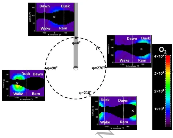
Figure 5: West longitude - latitude maps of the rate of O2 ejection (in O2/cm2/s) by sputtering at
various Ganymede phase angles. On each figure the X indicates the subsolar point whereas the vertical dashed lines represent the terminators labeled accordingly as dawn and dusk. Also indicated on each panel are the positions of the wake and ram hemispheres.
Due to the thermal inertia of the surface, the role of the ram direction for the sputtering and the shape of the opened field lines region, there is a larger flux ejected close to the dusk than to the dawn when averaging over an orbit. The peak O2 source rate occurs around a phase angle of 90° (at 5×10⁸ O2/cm2/s) due to the variation in latitude of the opened/closed field lines boundary from the ram to wake hemispheres. At a phase angle of 90° the largest open field line region (wake
hemisphere) is also where the surface temperature is highest resulting in an enhanced sputtering efficiency according to equations (3) and (4). In contrast, at a phase angle of 270°, the opened field line region is smallest on the dayside (the ram hemisphere), leading to a globally lower rate of
ACCEPTED MANUSCRIPT
23
ejection (3×10⁸ O2/cm2/s). Sputtering ejection reaches a minimum at a phase angle of 0° (2.4×10⁸ O2/cm2/s) because of the eclipse induced by Jupiter’s shadow and the rapid decrease of Ganymede's surface temperature (Figure 1a). Since the modeled atmosphere is nearly stationary, a variation in the ejection or loss rate produces a variation in the total content of the O2 exosphere. Therefore, the total O2 content reaches a minimum around a phase angle of 20° due to the low ejection rate during the previous half of the rotation, between phase angles 200° to 20° with a peak around a phase angle of 150° following the maximum in ejection rate around a phase angle of 90°. That is, Ganymede's O2 exospheric total content decreases during a portion of its orbit centered around a phase angle of 330° where the loss rate due to electron impact ionization/dissociation is larger than the ejection rate. During this portion of the orbit, Ganymede's decaying exosphere is a residual that formed earlier and conversely, during the following portion of the orbit around a phase angle of 150°, the total content increases. The O2 exosphere also appears slightly more extended on the dayside (Figure 4) due to larger surface temperatures. In our model, O2 is mainly ejected from the higher latitudes by sputtering as explained in section II.4 (Figure 5). However, the vertical column density of the O2 clearly peaks at the equator (Figure 4b) and not at high latitudes. The O2 diffusion time suggests that the molecules remain close to their source regions. However, this does not take into account the effect of the centrifugal force which tends to drive molecules equatorward. This force has an average intensity equal to few percent of Ganymede's gravitational force at the surface and can therefore, shape the O2 exosphere as seen in Figure 6a. The observed dusk/dawn asymmetry seen in Figure 4a leads also to larger column density on the right (dusk) side of the exosphere as seen from the Sun in Figure 6a. This dusk/dawn ratio in the O2 column density peaks at a value of 3.4 at a phase angle of 150°. Ganymede’s exosphere near the leading hemisphere portion of the orbit is formed by the production and spreading of the high latitude ejecta as seen from Figure 5. The dusk/dawn
asymmetries simulated here are also produced when simulating the orbital evolution of Europa’s O2 exosphere using the EGM (Oza et al. 2016), in accordance with recent HST orbital observations of auroral features there (Roth et al. 2016)
ACCEPTED MANUSCRIPT
24
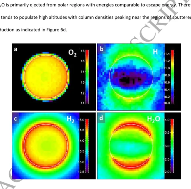
The H exosphere is produced from the polar region by sputtering in our model. The column density, as seen from the Sun shown in Figure 6b, reflects the source region and that the ejection energy primarily leads to escape. Sputtered H2, on the other hand, is ejected at the local surface
temperature at lower energies, and with its higher mass a significant fraction remains gravitationally bound. Since it does not stick, a nearly isotropic H2 exosphere results as shown in Figure 6c (despite electron and photon impact dissociation of H2). In the low-sublimation scenario presented in Figure 6, H2O is primarily ejected from polar regions with energies comparable to escape energy. Therefore H2O tends to populate high altitudes with column densities peaking near the regions of sputtered production as indicated in Figure 6d.
Figure 6: Reconstructed column densities (in log10 cm-2) of the O2 exosphere (panel a), of the H
exosphere (panel b), H2 (panel c) and H2O (panel d) at a phase angle of 270° as seen from the Sun.
We also tested if the formation of a surface reservoir by the readsorped H2O test-particles
ACCEPTED MANUSCRIPT
25
is the main component of the surface, we did not notice any effect associated with the formation of an exospheric reservoir of H2O in the surface.
III.2 The role of collisions
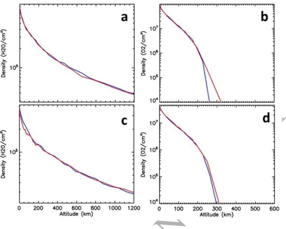
As suggested by Marconi (2007), Ganymede's atmosphere might be locally collisional. We therefore investigated the effect of momentum transfer collisions on the global distribution of the exosphere. Since the implementation of collisions, requires of the order of a few weeks on 128 CPUs, we only ran simulations on one phase angle. Starting from the steady-state solution calculated in the collisionless regime (as described in section III.1), we simulated the fate of Ganymede's exosphere, including collisions (section II.5), during a time period long enough (few tens of hours) to reach an accurate description of the exosphere up to 1200 km in altitude. In Figure 7, we compare the density profile of the two main components in Ganymede's exosphere with and without taking into account the effects of collisions at a phase angle of 90°.
As shown in Figure 7, the main effect of collisions on the density profile is to enhance the population of O2 at high altitudes. Indeed, most of the collisions occur either between O2 molecules or between O2 and H2O molecules, the two main species in the collisional region near the surface (within the first tens kilometers). In this layer, collisions between other thermal O2 molecules have a negligible effect on the O2 radial density distribution. However, O2 collisions with the more energetically sputtered H2O possessing a high energy tail (1/E²) can add significant energy to the O2 molecules, thereby expanding the O2 exosphere.
ACCEPTED MANUSCRIPT
26
Figure 7: Density profiles simulated by EGM without collision (blue lines) and with collision (red lines) as calculated at a phase angle of 90°. Panels a and b are for H2O and O2 exospheric species
respectively at the subsolar point whereas panels c and d are for H2O and O2 exospheric species
respectively at the polar region. The density profile is calculated as the average density within 10° of the subsolar point (panels a and b) and to the North pole (panels c and d).
We find that our results are in good agreement with the conclusions by Shematovich (2016) model of Ganymede’s exosphere. This author found that collisions caused the 10 to 100 km altitude region to be populated by both O2 and H2O. Similarly, Marconi (2007) suggested that charge exchange between O2+ ion and O2 molecules could enhance the population of O2 in the upper exosphere. Charge exchange was also investigated by Dols et al. (2016) and by Luchetti et al. (2016) at Europa who both suggested that charge exchange between O2+ and O2 might be the dominant loss process for that satellite. Including charge exchange accurately requires coupling between a magnetospheric and an exospheric model, which is work in progress. The near surface density has a typical scale heights for O2 of 50 km which is significantly larger than the expected scale height, 27 km, for an
ACCEPTED MANUSCRIPT
27
atmosphere in thermal equilibrium with the surface at a maximum temperature of 146 K. In this model, O2 molecules are always ejected from the surface following a Maxwell-Boltzmann distribution defined by the surface temperature. However, as discussed in section III.1, O2 molecules are particularly sensitive to the non-inertial forces because of their long residence time in the atmosphere. A large portion of the O2 molecules come from regions far from the local surface leading to a globally uniform layer at the poles. This was illustrated in Turc et al. (2014) where the O2 density at the poles decreased much faster (with scale height around 22 km) than in the subsolar region.
III.3 The role of sublimation
For the Fray and Schmitt (2009) parametrization of sublimation, the total ejection rate would be equal to 3.5×1029 H2O/s (comparable to the 8.0×1027 H2O/s sputtered and to the 7×1029 H2O/s sublimated in Plainaki et al. (2015)). This implies that the H2O exosphere would be dominated by sublimation. This is clearly illustrated by simulation results in Figure 8a which displays the exospheric density in the equatorial plane, with the same format as in Figure 4a. The H2O density peaks as expected around the subsolar region with a clear shift towards the afternoon due to the shift of the maximum temperature on the dayside (Figure 1b). The eclipse period is particularly dramatic, since as shown by Turc et al. (2014), the quick decrease of the surface temperature (Figure 1a insert) leads to an almost complete disappearance of the H2O exosphere (characterized by a collapse of the density by more than 4 orders of magnitude). The extended part of the H2O exosphere (in longitude and altitude with density larger than 104 H2O/cm3) is due to the sputtering of polar regions by the incident Jovian plasma. It is clearly more important on the wake side of the satellite because sputtering occurs at significantly lower latitudes than on the ram side (Figure 3 and section III.1). As soon as a H2O molecule reaches the nightside, it sticks efficiently so that the H2O exosphere is essentially confined on the dayside. In this scenario, the exosphere at the equator is dominated by the H2O.
ACCEPTED MANUSCRIPT
28
Figure 8: Panel a: Vertical column densities (log10 cm-2) of the H2O exosphere at different Ganymede
phase angles (90°, 210°, 270° and 0°) with respect to latitude (vertical axis) and west longitude (horizontal axis) in the high sublimation scenario. The subsolar point is indicated by the white cross on each panel, the dusk and dawn terminators by vertical dashed black or white lines. The ram and wake hemispheric centers are also indicated. Ganymede’s direction of rotation is indicated by the counter-clockwise arrow in the plane of Jovian co-rotation. Jupiter is at the center of each figure. Panel b:
ACCEPTED MANUSCRIPT
29
Reconstructed column densities (in log10 cm-2) of the H2O exosphere at a phase angle of 90° (left
panel) and 270° (right panel) as seen from the Sun.
For a large sublimation rate, the typical LOS H2O column density (as seen from the Sun) would peak around the subsolar region with values between 3.1 and 8.5×10¹⁵ H2O/cm² (Figure 8b). The H2O sputtered from polar regions is also apparent in the Figure 8b. The slight asymmetry of the column density with respect to the subsolar point in Figure 8b is due to the maximum surface temperature occurring in the afternoon. Since dissociation of H2O is a minor source of H, the column density of H is very close (typically 4×10¹⁰ H/cm²) to that for the low sublimation rate case (in Figure 8b).
IV Discussion and Comparison with observations
Barth et al. (1997) reported a H column density of 9.21×1012 cm-2 in Ganymede's exosphere from the measured Lyman α emission of 0.56±0.2×10³ Rayleigh measured by Galileo during its G1 flyby (at a phase angle of 180° and a solar zenith angle of 60° with a latitude of 21°). Such emission intensity was later confirmed with HST (Feldman et al. 2000). The simulated H column density at that phase angle is on the order of 6×10¹⁰ H/cm2 in the polar region and is extended down to latitudes of 20° because of the particular shape of the open field line boundary at that particular phase angle. Our calculated column density is therefore two orders of magnitude lower than the estimated column density by Barth et al. (1997). A two order of magnitude error in the efficiency sputtering H atoms is difficult to imagine based on measured sputtering yields (Johnson et al. 2009).
In combination with resonant scattering, H2O dissociated via electron impact could be an additional channel producing Lyman α emission. Considering an electron with an energy near 20 eV, the typical cross section for the production of Lyman α by electron impact on H2O is 0.43×10⁻¹⁸ cm2 (Makarov et al. 2004). While trace ~keV hot electrons are a negligible contribution, an accurate knowledge of the
ACCEPTED MANUSCRIPT
30
core electron energy is particularly important since this cross section increases by one order of magnitude at 50 eV and peaks at 7×10-18 cm2 at 100 eV. Using the cross section at 20 eV, the typical column density of 1014 H2O/cm2 in the low sublimation scenario (Figure 6) and 1016 H2O/cm2 in the Fray and Schmitt (2009) sublimation scenario would lead to an emission of few Rayleigh and few hundred Rayleigh respectively. The Fray and Schmitt (2009) sublimation scenario would therefore be in rough agreement with Galileo-observed Lyman α emission. The low sublimation scenario could fit the observation for 40 eV core electron temperatures if the sputtering yield was ten times larger. A further potential source of Lyman alpha emission from Ganymede's exosphere is electron impact dissociation of H2, also suggested by Marconi (2007). Ajello et al. (1995) published a cross section for the production of Lyman alpha emission from electron impact dissociation of H2 peaking at 7×10-18 cm2 at 60 eV and equivalent to 5×10-18 cm2 at an electron energy of 20 eV. Using the typical 2×10¹⁴ H2/cm2 column density we simulated, this process would contribute less than a few tens of Rayleigh.
The typical column density of the O2 exospheric component has been reported by Hall et al. (1998) as being between 2.4×10¹⁴ and 1.4×10¹⁵ O2/cm² when observing Ganymede’s trailing hemisphere in June 1996 (phase angle around 270°) and by Feldman et al. (2000) as being equal to 0.3 to 5×10¹⁴ (October 30, 1998 with a phase angle between 290° and 300°). McGrath et al. (2013) also showed the spatial distribution of the auroral emission at different orbital positions characterized by localized bright regions with peak brightnesses between 100 to 400 Rayleigh in good agreement with the previous reported observations. As stated in Section II.4, the O2 sputtering yield was tuned in order to reproduce the reported column density. We therefore simulated column densities varying from 5 to 6.5×10¹⁴ O2/cm² averaged over the disk as observed from the Sun, and peaking to values of 2×10¹⁵ O2/cm² at the equatorial limb (Figure 6a).
ACCEPTED MANUSCRIPT
31
We also reconstructed the auroral emission associated with our simulated column density (Figure 9), by considering electron excitation by a uniform mono-energetic electron population impacting the sputtered O2 in the Alfven wings of Ganymede’s magnetosphere (open field line regions displayed in Figure 3) as the primary emission mechanism. We did not attempt to reproduce the ring shape emission in Feldman et al. (2000), McGrath et al. (2013), and Saur et al. (2015). Furthermore, we did not consider an accurate description of the electric currents in the open field line regions as in Payan et al. (2015). The electron population used to calculate the emission brightness is the same as earlier: an electron number density of 70 cm-3 and average energy of 20 eV. The emission rate coefficient for the production of OI (5So) atoms from O2 emitting photons at 135.6 nm wavelength is set to be 1.1×10⁻⁹ cm-3 s-1 as in Hall et al. (1998). The 135.6 nm emission produced by direct excitation of the O atoms by electron impact is also included, but is much smaller than the O2 source, in good agreement with Hall et al. (1998). The goal of our calculation is to look for any potential signature in the
observed auroral emission induced by the dusk/dawn asymmetry of the O2 exosphere (Figure 4). As shown in Figure 9, the simulated emission intensities vary between 10 and 200 Rayleigh in good agreement with the observed values. More interestingly, at a phase angle of 90° (panel a),
Ganymede's dusk exosphere is simulated as being up to two times denser than at dawn consistent with the column density of the O2 exosphere as seen from the Sun being 2.3 times larger on moon's esatern/dusk hemisphere with respect to the column density on the western/dawn hemisphere. This dusk/dawn asymmetry is visible in the simulated emission brightness, the dusk limb emission at mid-latitudes being significantly larger than the dawn limb emission. Remarkably, a similar asymmetry between the dawn and dusk limbs was reported by HST (panel a of Figure 2 in McGrath et al. 2013). At a phase angle of 270° (Figure 9, panel b), the simulated dawn/dusk asymmetry is much smaller (the west/dawn to east/dusk hemispheric average column density ratio begin equal to 1.3), and does not induce a significant emission asymmetry (Figure 9b), as is also seen with HST observations (panel c of Figure 2 in McGrath et al. 2013). As indicated by HST observations near the trailing hemisphere (Fig. 9b) the auroral emissions occur at higher latitudes than at leading (Fig. 9a) since we are facing
ACCEPTED MANUSCRIPT
32
the ram hemisphere where the open/closed field lines boundary is also shifted to higher latitudes (Fig. 3). The third position reported in McGrath et al. (2013) at a phase angle of 350° (their Figure 2b; near eclipse) is characterized by two bright spots on the right limb. Our simulated image only
marginally reproduces such an intense asymmetry between right and left hemispheres (the right to left column densities ratio being equal to 1.2). However, this observation was partially reproduced by Payan et al. (2015) in their Figure 1 using a homogeneous exosphere coupled to a 3D MHD simulation of Ganymede's magnetosphere, suggesting that these bright spots at the limb might be partly due to the current system in Ganymede's magnetospheric Alfven wings. Payan et al. (2015) provided a similar comparison for the two other observed positions (Figures 9a and b) and noted that the bright spot at a phase angle of 105-108° (Figure 9, panel b) could not be reproduced. We suggest here, that this bright spot may be a signature of the strong dusk/dawn asymmetry at the leading
hemisphere/plasma wake. Additionally, this dusk/dawn asymmetry could contribute to the almost systematic right to left brightness asymmetry observed in the auroral emissions (McGrath et al. 2013; Saur et al. 2015).
ACCEPTED MANUSCRIPT
33
Figure 9: Simulated images of the HST observed emission brightness reported in McGrath et al. (2013) at three different phase angles as indicated on each panel with emission brightness calculated as explained in the text.
Using the emission rate coefficient for the 130.4 nm emission, the typical ratio between 135.6 nm and 130.4 nm is equal to 1.8 with decreasing values at the edge of the emission region where the O/O2 relative abundance tends to increase. Hall et al. (1998) and Feldman et al. (2000) reported ratios between 1.2 and 3.2.
Teolis et al. (2016) suggested that the radiolysis efficiency to sputter O2 molecules from an icy surface might be between 50-to-300 times less efficient than predicted by laboratory experiments (Teolis et al. 2010) or as calculated by Cassidy et al. (2013). In this paper, we scaled this efficiency to reproduce
ACCEPTED MANUSCRIPT
34
the observed O2 column density and found that the ejected O2 rate should be around 3.4×1026 O2/s, assuming a flux of Jovian ions precipitating on Ganymede's surface between 3.3 and 3.7×1024 particles/s for the thermal component (Leclercq et al. 2016) and ~1024 particles/s for the high-energy component (Fatemi et al. 2016), leading to an average sputtering yield of 100. Teolis et al. (2016) estimated the yield for ion sputtering on the icy satellites Rhea or Dione to be between 0.01 and 0.03, 4 orders of magnitude less than the yields inferred in this paper. The temperature difference between Rhea, Dione, and Ganymede could only account for a factor of 10 larger. Since an ion precipitation rate that is two orders of magnitude larger is not realistic, we note that the Jovian plasma is more energetic with respect to the Saturnian plasma (Teolis et al. 2016). Such a difference in energy could also lead to an additional order of magnitude larger efficiency at Ganymede than at Dione or Rhea, leaving a difference of two orders of magnitude with respect to the conclusions of Teolis et al. (2016). This difference is re-enforced by noting that two orders of magnitude smaller O2 column density would place atomic products below the detection limit of FUV oxygen aurorae observations by HST. Teolis et al. (2016) also suggested that for reproducing Rhea’s exosphere evolution, it was needed to introduce the notion of a shallow 1-cm regolith allowing for the diffusion of O2 into the regolith and its shielding from the impacting ions. The release of the O2 is then allowed when the regolith rotates into sunlight and induces the diffusion of the O2 molecules back to the surface where they can be released by sputtering. Applied to Ganymede’s case, such a process would increase the reservoir of O2 available for ejection (by desorption or sputtering) and therefore help reconcile Teolis et al. (2016) sputtering efficiency and the efficiency inferred by our modelling. It would imply that more than 99% of the O2 originally produced by radiolysis accumulates in the regolith over time and is released into the exosphere by thermal desorption and/or direct sputtering. In such a scenario, the O2 exosphere would be much more extended in longitude and latitude. We should also expect a much less asymmetric dawn to dusk terminator, in which the O2 exosphere behaves like the H2O exosphere. Moreover, given that O2 is more efficiently adsorbed and trapped inside the regolith than simulated here, a dawn enhancement would be favored by the release of
ACCEPTED MANUSCRIPT
35
trapped O2 at sunrise and a decrease in reservoir content with increasing solar zenith angle. O2 trapping in the regolith has actually been suggested by ground-based observations peaking at the trailing hemisphere (Spencer et al. 1995), and confined at the equatorial regions (Calvin and Spencer 1997). It was shown by Johnson and Jesser (1997) that O2 (and O3) bubbles can be trapped as voids in Ganymede’s regolith with the caveat that they can be destroyed should the incident ion flux be too high. The absence of O2 at the poles, as well as the significantly less O2 at the leading hemisphere/plasma wake might be explained by a more efficient eroding of the trapped O2 bubbles by the incident plasma.
V Conclusions
In this paper, we present the first model of Ganymede's exosphere taking into account Jupiter’s gravitational influence and the evolution of Ganymede's exosphere along its orbit around Jupiter. This 3D Monte Carlo model takes into account sublimation and sputtering as the main processes of ejection, electron impact ionization and dissociation in the exosphere as well as a detailed interaction between the exosphere and the surface. The role of Ganymede's magnetosphere is described in a simple way which allows us to clearly distinguish signatures associated with the magnetosphere to those associated with the formation and evolution of the exosphere. Ganymede's exosphere appears to be highly stratified, displaying significant structure in terms of density and composition due to the variation of the ejection mechanisms and molecular movement over its orbital period. In particular, our results suggest that the shape of Ganymede's O2 exosphere at a given orbital position is highly dependent on the production earlier in its orbit. We also showed that the H2O exosphere is very different for the high sublimation rate and a low sublimation rate models. Moreover, even if Ganymede's atmosphere is quasi-collisional, collisions are shown to only have a minor effect on the exospheric density distribution.
ACCEPTED MANUSCRIPT
36
In this work, we show that, by observing Ganymede's multi-species, water product exosphere along its orbit, significant information on the way Ganymede interacts with its environment should be accessible:
- The formation of the exosphere is a complex process driven by the impacting plasma and the resulting space weathering of the surface, whose efficiency depends on the surface characteristics (e.g. temperature, composition, structure) and on the Jovian plasma parameters (e.g. flux, energy and spatial distribution at the surface). The spatial distribution for the lighter species of the sputtered exosphere should directly reflect the spatial characteristics of the interaction between Ganymede and Jupiter’s magnetosphere. Moreover, the sputtered exospheric temporal variability and composition should be highly dependent on the surface temperature and composition and could therefore be used to constrain these two surface properties.
- The global 3-D spatial distribution of the exospheric density will depend on the influence of Jupiter and Ganymede’s gravitational fields. The fate of the ejecta is also species-dependent due to the species dependent surface interactions. As an example, the dusk/dawn asymmetry in O2 highlighted in this paper depends on the mobility across Ganymede’s surface affected by absorption,
accumulation and re-emission from the regolith. The observed spectral emission signatures, such as the auroral emissions, could be potentially used to characterize not only the Jovian-Ganymede interaction (Saur et al. 2015), but also the spatial distribution of the exosphere.
- Ultimately, tracking the evolution of Ganymede's exospheric morphology and content along its orbit should help constrain its atmospheric formation, and the interaction of its magnetospheric plasma with the atmosphere and surface. The Galileo spacecraft showed the dichotomy in the surface albedo between the trailing and leading hemispheres, which suggest that, Ganymede's exospheric source can depend strongly on geographic longitude, an effect we did not consider in this work, but will implement in the future. To better constrain the full structure of the exosphere we suggest full
ACCEPTED MANUSCRIPT
37
orbital observations of Ganymede’s FUV oxygen aurorae capable of indicating the evolution of Ganymede’s atmosphere.
Acknowledgement: This work is part of HELIOSARES Project supported by the ANR
(ANR-09-BLAN-0223) and ANR MARMITE-CNRS (ANR-13-BS05-0012-02). Authors are also indebted to the "Système Solaire" program of the French Space Agency CNES for its support. Authors also acknowledge the support of the IPSL data center CICLAD for providing us access to their computing resources and data. Data may be obtained upon request from F. Leblanc (email:[email protected]).
References
Abramov O. and J.R. Spencer, Numerical modeling of endogenic thermal anomalies on Europa, Icarus, 195, 1, 378-385, 10.1016/j.icarus.2007.11.027, 2008
Ajello J.M., Kanik I., Ahmed S.M. and J.T. Clarke, Line profile of H Lyman α from dissociative excitation of H2 with application to Jupiter, J. Geophys. Res. et al., 100, E12, 26411-26420, 1995
Barth, C.A., Hord, C.W., Stewart, A.I.F., Pryor, W.R., Simmons, K.E., McClintock, W.E., Ajello, J.M., Naviaux, K.L. and Aiello, J.J.: Galileo ultraviolet spectrometer observations of atomic hydrogen in the atmosphere of Ganymede, Geophys. Res. Lett., 24, 2147–2150, 1997
Bird, G. A., Molecular Gas Dynamics and the Direct Simulation of Gas Flows, Clarendon, Oxford, England, 1994.
Calvin W.M. and J.R. Spencer, latitudinal distribution of O2 on Ganymede: Observations with the Hubble Space Telescope, Icarus, 130, 505-516, 1997.
Cassidy, T.A., Paranicas, C.P., Shirley, J.H., Dalton, J.B., I.I.I., Teolis, B.D., Johnson, R.E., Kamp, L., Hendrix, A.R., Magnetospheric ion sputtering and water ice grain size at Europa, Planet. Space Sci., 77, 64–73, http://dx.doi.org/10.1016/j.pss.2012.07.008, 2013.
ACCEPTED MANUSCRIPT
38
Cooper, J.H., R.E. Johnson, B.H. Mauk and N. Gehrels, Energetic ion and electron irradiation of the icy Galilean satellites, Icarus, 149, 133, 2001.
Dols, V., Bagenal, F., Cassidy, T., Crary, F., Delamare, P., Europa’s atmospheric neutral escape: importance of symmetrical O2 charge exchange, Icarus, 264, 387–397,
http://dx.doi.org/10.1016/j.icarus.2015.09.026, 2016.
Eviatar A., Vasyliunas V.M. and D.A. Gurnett, The ionosphere of Ganymede, Planet. Space. Sci., 49, 327-336, 2001a.
Eviatar, A., Strobel, D.F., Wolven, B.C., Feldman, P.D., McGrath, M.A., Williams, D.J., Excitation of the Ganymede aurora. Astrophys. J. 555, 1013–1019, 2001b.
Fatemi, S., Poppe, A. R., Khurana, K. K., Holmstrm, M., Delory, G. T., On the formation of Ganymede's surface brightness asymmetries: Kinetic simulations of Ganymede's magnetosphere: plasma
interaction with Ganymede, Geophys. Res. Let., 43, 4745, http://doi.wiley.com/10.1002/2016GL068363, 2016.
Feldman, P.D., McGrath, M.A., Strobel, D.F., Warren Moos, H., Retherford, K.D., Wolven, B.C., HST/STIS ultraviolet imaging of polar aurora on Ganymede. Astrophys. J. 535, 1085–1090, 2000.
Fama, M., Shi,J., Baragiola, R.A., Sputtering of ice by low-energy ions, Surface Sci., 602, 156–161, 2008.
Frank, L.A., Paterson, W.R., Ackerson, K.L., Bolton, S.J., Outflow of hydrogen ions from Ganymede. Geophys. Res. Lett., 24, 2151–2154, 1997.
Fray, N., Schmitt, B., Sublimation of ices of astrophysical interest: A bibliographic review. Planet. Space Sci. 57, 2053–2080, http://dx.doi.org/10.1016/j.pss.2009.09.011, 2009.