HAL Id: insu-01276775
https://hal-insu.archives-ouvertes.fr/insu-01276775
Submitted on 4 Sep 2020
HAL is a multi-disciplinary open access
archive for the deposit and dissemination of
sci-entific research documents, whether they are
pub-lished or not. The documents may come from
teaching and research institutions in France or
abroad, or from public or private research centers.
L’archive ouverte pluridisciplinaire HAL, est
destinée au dépôt et à la diffusion de documents
scientifiques de niveau recherche, publiés ou non,
émanant des établissements d’enseignement et de
recherche français ou étrangers, des laboratoires
publics ou privés.
Patrick H. M. Galopeau, Mohammed Yahia Boudjada
To cite this version:
Patrick H. M. Galopeau, Mohammed Yahia Boudjada. An oblate beaming cone for Io-controlled
Jovian decameter emission. Journal of Geophysical Research Space Physics, American Geophysical
Union/Wiley, 2016, 121 (4), pp.3120-3138. �10.1002/2015JA021038�. �insu-01276775�
An oblate beaming cone for Io-controlled
Jovian decameter emission
P. H. M. Galopeau1and M. Y. Boudjada2
1LATMOS, Université Versailles Saint-Quentin-en-Yvelines, CNRS, INSU, IPSL, Guyancourt, France,2Space Research
Institute, Austrian Academy of Sciences, Graz, Austria
Abstract
We investigate the emission cone of the Io-controlled Jovian decameter radiation from the layout of the sources in the central meridian longitude (CML)-Io phase diagram where the occurrence of the radiation is plotted versus the central meridian longitude (CML) and the phase of the satellite Io. Four zones of enhanced probability are revealed in this diagram and named Io-controlled sources Io-A, Io-B, Io-C, and Io-D. We propose an angular representation of the CML-Io phase diagram in a coordinate system linked to the local magnetic field in the radio source and the gradient of the magnetic field. The angular distribution of the sources in such a diagram clearly shows that the radio emission is radiated in a hollow cone which is not axisymmetrical around the magnetic field gradient but flattened in the direction of the magnetic field vector. The use of elliptic coordinates allows us to compute the variable opening angle and the flattening of the cone in both Jovian hemispheres. Finally, it comes from our investigation that the flattening of the emission cone allows the theoretical existence of a Jovian active longitude sector much more easily than in the case of an axisymmetrical cone, and the zones of maximum theoretical amplification correspond to the areas of high occurrence probability observed in the CML-Io phase diagram.1. Introduction
More than a half-century ago, Burke and Franklin [1955] discovered that the planet Jupiter was a strong intermittent source of radio-frequency energy in the decameter (DAM) wavelength. This DAM radiation is pro-duced in Jupiter’s magnetosphere and extends from a few megahertz to 40 MHz. The high intensity and the rapid variations, both in time and frequency, of this radiation are characteristic of a nonthermal mechanism. Four other magnetized planets in the Solar System (the Earth, Saturn, Uranus, and Neptune) are known to present similar radiations. In the following, we focus on a particular radiation of Jupiter: the Io-controlled DAM emission, the occurrence probability of which depends on both the Jovicentric longitude of the observation point and the phase of the satellite Io. This study follows a series of earlier publications on the existence of an active longitude of Jupiter favoring the radio emission. The present paper is devoted to the emission pattern of the DAM which is usually considered as a hollow cone with a rotational symmetry; we show that, instead, the emission cone is flattened in a specific direction in relation to the magnetic field.
In the next section, we detail the specific features of the Jovian decametric emissions and the ground-based long-term observations which provide observational constraints on the context of the wave generation. Then we address the problems related to the conditions of propagation and beaming, and the underlying assumptions that are usually considered. In section 3, we study the angular distribution of the regions of high occurrence probability and its consequences on the beaming cone. In section 4, we discuss the implications of the flattening of the cone. Then we present the conclusions we can draw from our study.
2. Outline of the Problem
2.1. Characteristics of the Jovian Decametric Emission
The Jovian decametric radiation is produced in Jupiter’s magnetosphere and extends from a few megahertz to 40 MHz. This planetary radio emission is the only one which can be observed from ground-based stations. Jupiter can be tracked daily 8 h (4 h before and after the local meridian) throughout the year. The obser-vations are often limited to the nighttime hours because of terrestrial interferences which are particularly important during the daytime. A low-frequency limit around 10 MHz, and may be as low as 5 MHz, is due to the ionospheric cutoff. A catalog of regular observations can be made which gives a list of several parameters
RESEARCH ARTICLE
10.1002/2015JA021038
Key Points:
• First evidence for a flattening of the Jovian decameter emission cone • Angular representation of CML-Io
diagram
• Existence of Jovian active longitude sector
Correspondence to: P. H. M. Galopeau,
Citation:
Galopeau, P. H. M., and M. Y. Boudjada (2016), An oblate beaming cone for Io-controlled Jovian decameter emission, J. Geophys. Res. Space Physics, 121, 3120–3138, doi:10.1002/2015JA021038.
Received 20 JAN 2015 Accepted 17 FEB 2016
Accepted article online 19 FEB 2016 Published online 15 APR 2016
©2016. American Geophysical Union. All Rights Reserved.
like the beginning and the end of the emission, the corresponding central meridian longitude (CML) and Io phase, and also the receiver frequency range and emission bandwidth. Such a catalog provides an overview of the occurrence probability of the Jovian decametric emission [e.g., Boudjada and Leblanc, 1992]. Most of the powerful Jovian decametric radiations are observed at some specific positions in relation to the rotating planetary magnetic field and the satellite Io [Bigg, 1964]. The occurrence of the emission is usually displayed in the so-called CML-Io phase diagram, which reveals several areas of enhanced occurrence probability named Io-controlled sources: Io-A, Io-B, Io-C, and Io-D [Carr et al., 1983]. They are associated with emission coming from the Northern or the Southern Hemisphere according to their polarization features. Hence, Io-A/Io-B and Io-C/Io-D radiations are mainly elliptically polarized in the right-hand and left-hand senses, respectively [Lecacheux et al., 1991]. The associated emission beam is considered to have the form of a hollow cone with apex at the point of emission and axis tangent to the magnetic field direction. The half-angle of this hollow cone was estimated to be ∼80∘ [Dulk, 1965].
The Io-controlled beamed emissions are associated with sources along or near the Io flux tube (IFT). Hence, the right-hand polarized emissions (mainly Io-A and Io-B) are produced along flux tubes which intersect Io’s orbit a few tens of degrees ahead or behind this satellite. Thieman and Smith [1979] fitted the statistical occur-rence of the emission by an apparent displacement of the flux tube 20∘ ahead of the orbital position of Io.
Genova and Aubier [1985] combined the observed high-frequency limit of the emission with those deduced
from the O4 magnetic field model. They showed that the Io-controlled emissions of the Northern Hemisphere are produced along flux tubes which intersect Io’s orbit, on average, 70∘ behind Io. Later, Wilkinson [1989] investigated the Io-related Jovian decametric arcs and developed a geometrical model where the Io source regions are carried on magnetic field lines corotating with Jupiter. Menietti and Curran [1990] performed a ray tracing analysis of the Jovian Io-controlled DAM emission. They found that the radiation is produced close to the gyrofrequency along field lines that are within 20∘ of the instantaneous Io flux tube. The authors showed that the O4 model, used by Genova and Aubier [1985], may introduce a discrepancy of about 38% in the maximum allowed frequency.
2.2. Emission Cone Model 2.2.1. Jovian DAM Radiation
Dynamic spectra from ground-based and Voyager observations have revealed that the patterns of Jovian decametric emission on the time-frequency plane can be resolved into families of arcs somewhat like groups of nested opening or closing parentheses. Several authors have proposed models in which each spectral arc geometrically results from the rotation of families of hollow cone beams of different frequencies threaded by an activated flux tube [Goldstein and Thieman, 1981; Leblanc, 1981; Pearce, 1981]. This suggests that the spectral arcs of Io-A and Io-B may be approximated by a large number of thin conical surface beams, the apexes of which are distributed over a limited range of longitudes, and the axes of which are parallel to the magnetic field. However, observations over a large frequency band (2 MHz–36 MHz) showed the necessity to assume the presence of refraction effects taking place near the source region [Lecacheux et al., 1998]. The authors explained the discrepancy as a refraction effect of the radio waves at grazing incidence on the “radio horizon” above the planetary limb. The concept of an emission beamed in a hollow cone, as suggested by
Dulk [1965], is mainly based on observations recorded at a far distance from the planet; it is the case for Jupiter
and also the other giant planets. The geometrical coverage of the emission beam is limited to some tens of degrees, and the exact location of the sources of the DAM radiation is poorly known. It is generally accepted that the emission mechanism is the cyclotron maser instability [Wu and Lee, 1979] which implies that the frequency of the emission f is close to the cutoff frequency fXof the X mode: f ≃ fX≃ fc(1+fp2∕f
2
c) where fpand
fcare the plasma frequency and the gyrofrequency, respectively. In the Jovian magnetosphere, the condition
fp≪ fcis always fulfilled. As a consequence, the source is located quite close to the surface of Jupiter, and the
radiation is emitted at a large angle relative to the local magnetic field line. The Io-controlled emissions are defined by specific areas in the CML-Io phase diagram corresponding to a high occurrence probability, but the associated radio sources do not necessarily correspond to distinct locations in the Jovian magnetosphere. Another method used for the DAM source location is the ray tracing technique which implies numerous solu-tions for the source regions. The way to limit their number is to use constraints derived from a prior knowledge of the generation mechanism and to take into account the beaming characteristics of the emission. Hashimoto
and Goldstein [1983] were the first to investigate the observed occurrence probability of the Io-controlled
radiation using a three-dimensional ray tracing method. They found that the occurrence asymmetry in the CML-Io phase diagram is caused by the effect of Alfvén waves which are more intense when propagating
southward than northward. Menietti et al. [1984a, 1984b] extended the previous work by studying the arc structures using a three-dimensional ray tracing program. The inputs are mainly related to the source posi-tion like the radial distance, the longitude, and the latitude. The authors showed that the arcs present a low curvature and an upper cutoff frequency beyond 35 MHz when the CML ranges in the interval 90∘ –230∘, whereas they display a higher curvature and a lower upper cutoff frequency when the CML extends in the range 240∘ –80∘. These authors concluded that the B field structure that produces source points at the foot of the Io flux tube ranging in latitude from 45∘ to 70∘ and in altitude from 0 to 2 RJ produces noticeable
differences in the arc shape.
2.2.2. Terrestrial Auroral Kilometric Radiation Emission
Since the generation process of the planetary radio emissions is attributed to the same mechanism, i.e., the cyclotron maser instability, the Earth’s auroral kilometric radiation (AKR) is expected to exhibit a hollow pattern. Several satellites crossed the source regions where the AKR emissions occurred and provided a full coverage in longitude and in latitude of the source regions. Studies showed that the intense kilometric radi-ation generated over the nightside auroral zones is beamed into a cone-shaped region [Green et al., 1977], the radiation is generated in the extraordinary mode just above the local cutoff frequency and emanates nearly perpendicular to the magnetic field [Benson and Calvert, 1979], and the beaming could be explained by emission initially perpendicular to the magnetic field and wave refraction quite near the source [Calvert, 1981]. These results were confirmed by Viking observations where the AKR was found to be generated within strongly magnetized regions and to propagate outside the sources in a direction rather perpendicular to the geomagnetic field [Louarn and Le Quéau, 1996].
A statistical description of the AKR sources showed that the emission is generated in regions with small transverse scales, typically 100 km [Hilgers et al., 1991], and the AKR cavities extend from 30 km to 300 km in latitude [Ergun et al., 1998]. Statistical studies over 2 years allowed to show the character of the AKR global directivity. Kuril’chik et al. [2006] found that the intense AKR is more often observed in the magnetic local time (MLT) intervals 00:00–16:00 MLT for the Southern Hemisphere, and 00:00–05:00 MLT and 14:00–20:00 MLT for the Northern Hemisphere. In particular, the authors noted that the cones of emission of many appearing “elementary” sources were overlapped creating the total distribution of an ellipse form for both hemispheres. Using Cluster observations, Mutel et al. [2004] described, for the first time, a new technique to directly deter-mine the location of auroral kilometric radiation bursts using very long baseline interferometry (VLBI). The authors showed that the AKR sources were localized in the evening sector of the Northern Hemisphere. The mean magnetic local times and the corresponding invariant magnetic latitudes varied, respectively, between 18.2 h and 20.7 h and between 68.4∘ and 71.0∘. The AKR location footprints in the Southern Hemisphere were found to be significantly shifted compared with the Northern Hemisphere locations with mean magnetic local times close to midnight or in the morning sector, i.e., from 22.7 h to 22.1 h, and mean invariant magnetic latitudes between −71.7∘ and −75.1∘. Also, through recent investigations, Mutel et al. [2008] revealed that the individual bursts associated to AKR emission do not radiate in hollow cones but are rather confined to a plane sheet containing the local magnetic field vector and perpendicular to the great circle connecting the mag-netic poles. They showed, in particular, that AKR observations from remote locations sample only a small part of the auroral oval from any given location.
2.3. Active Longitude Sector
The regular monitoring of the Jovian decametric emissions allowed to find in the CML-Io phase diagram enhancements of occurrence probability for given Io phases (near 90∘ and 240∘). Another important charac-teristic of this diagram is the occurrence dependence on the central meridian longitude. Two enhancements are observed in the CML intervals 90∘ –180∘ and 200∘ –300∘. These longitude enhancements suggest the presence of an “active sector” which was investigated by Galopeau et al. [2004] who proved that the existence of such a longitude sector can be explained by the cyclotron maser instability (CMI). The starting point was the calculation of the growth rate of the waves derived from the CMI theory versus the Jovicentric longitude of Io. The maximum growth rate was supposed to correspond to a strong occurrence probability of the radi-ation taking into considerradi-ation the following hypotheses. First, the cyclotron maser instability is at the origin of the waves which are emitted within a hollow cone at the local gyrofrequency, the source of free energy is a loss cone distribution function built up by electrons. We make the hypothesis that these electrons, after being accelerated in the vicinity of Io, follow an adiabatic motion along the magnetic field lines linked to the satellite. Their disappearance probability in the Jovian ionosphere is expected to be proportional to the length of their actual path and to the ionospheric density. Also, these electrons at the origin of the radiation are
supposed to have a Maxwellian distribution function by Io’s orbit, whereas the distribution function remains constant along the magnetic field line toward Jupiter. On the other side, the theory of CMI in a homogeneous medium has to be used rather than the theory in an inhomogeneous medium because the decameter wave-lengths𝜆DAM∼ 15 m (at 20 MHz) are much smaller than the typical length scale of the Jovian magnetic field
LB= B∕‖∇B‖ ∼ 18,000 km so that the electrons can interact with the unstable waves during a large number of periods. Finally, the main result of this study was that the efficiency of the cyclotron maser instability was max-imum around 130∘ and 200∘ for the Northern and Southern Hemispheres, respectively [see Galopeau et al., 2004, Figure 7].
Another important result was the working out of a theoretical CML-Io phase diagram based on the simulta-neous validity of two conditions: the radio emission can be observed only when the direction to the observer is located on the emission cone carried away by a magnetic field line, the footprint of which is located in an active longitude sector of Jupiter where the growth rate of the CMI is maximum. Then we have built a model of occurrence diagram consisting of four segments representing the visible zones of highest occurrence proba-bility as a function of the CML and Io phase [see Galopeau et al., 2004, Figure 9]. The modeled and the observed occurrence diagrams of DAM emissions were found to be fairly similar, in particular, with regard to the central meridian longitude. Afterward, in a second paper Galopeau et al. [2007a] proposed a parametric study of the theoretical location of the sources in the CML-Io phase diagram taking into consideration the lead angle of the active magnetic field line, the declination of the Earth, the half-angle of the emission cone, and the frequency of the radiation. An agreement was found between the modeled and the observed diagrams, in particular, when the lead angle is equal to 0∘ or 40∘ for the northern (Io-A and Io-B) or southern (Io-C and Io-D) sources, respectively. In a more recent paper, Galopeau and Boudjada [2010] present a new approach which consists in searching for the emission cone opening angle and active longitude from the observed CML-Io phase diagram. It is shown that the lead angle of the active magnetic field line relative to Io has a significant effect on both the selection of the propagation conditions and the limit between the right- and left-hand polariza-tion states. The modeled and observed occurrence regions are found to be similar for a lead angle of ∼20∘. Despite several common features between the modeled and observed diagrams, some discrepancies should be mentioned. First of all, it is not possible to simultaneously fit, in the modeled diagram, the correct occur-rence areas of the four Io-controlled sources at the same time. Also, one has to note that the polarization and the area of the occurrence regions of the southern hemisphere sources (Io-C and Io-D) are trickier. This inadequacy of the model indicates that the existence of an active longitude sector (mainly linked to Jupiter’s magnetic field) is probably not the only factor that rules the occurrence probability. Zaitsev et al. [2006] proposed that the electron density and energy might depend on the longitude of the satellite, so that we could expect the electron flux coming from Io to be another factor. The developed model rests on two essen-tial assumptions which might be questioned: a common active longitude range (linked to the efficiency of the emission mechanism) and a radiation beamed in a hollow cone.
3. Angular Distribution of the Source Regions
We have decided to reconsider some of the assumptions developed in the previous papers [Galopeau et al., 2004, 2007a; Galopeau and Boudjada, 2010] in order to obtain a better agreement between the model and the observations for both hemispheres. The emission was supposed to be beamed into a radiation pattern believed to have the form of a hollow cone with apex at the point of emission and axis tangent to the magnetic field direction. In the next subsection, we concentrate on the definition of the emission cone axis in order to give a better account of the wave propagation in the source.
3.1. Emission Cone Axis
The axis of the emission cone has always been taken along the direction of the local magnetic field, thus, tangent to the field line crossing the source region. This choice was justified by the observations of the radio emission, in particular, the arc structures that appear in the dynamic spectra. From the beginning, the CMI theory involves the local magnetic field B for the calculation of the resonance between the electronic popu-lation of the plasma and the growing waves in a homogeneous medium where B is uniform. Le Quéau et al. [1985] have elaborated a theory of the cyclotron maser instability in an inhomogeneous medium where, for simplification’s sake, all the gradients (∇B = ∇(‖B‖) for the magnetic field and ∇n for the electronic density) are along the direction of the vectorial field B. On the other hand, the authors consider that the plasma is constituted of a cold component which supports the wave propagation and a nonthermal energetic
(hot) component which may take part in the instability, independent of the cold plasma, when the resonance condition is fulfilled. The ray path of the wave through the source region is determined by the spatial variation of the index N = kc∕𝜔 (with the usual notations) in the cold plasma, so that the emergence angle of the wave (out of the source region) is defined relatively to ∇N which constitutes the equivalent of an “optical axis.” ∇N depends on both ∇n and ∇B. In this paper, we consider a situation more general than that proposed by Le
Quéau et al. [1985] by assuming that ∇n and ∇B are not along B. In the following, we focus on the X mode,
which is predominantly favored by the CMI, and we suppose that the propagation is quasi-perpendicular, which does not change the general nature of the problem.
The X-mode cutoff frequency of the X mode is
𝜔X= 𝜔c 2 + ( 𝜔2 c 4 +𝜔 2 p )1∕2 , (1)
where𝜔c = 2𝜋fc = eB∕m and𝜔p = 2𝜋fp = (ne2∕m𝜖0)1∕2stand for the gyrofrequency and the plasma frequency of the cold component of the electronic population.
The refractive index of the X mode, at the frequency𝜔 = 2𝜋f in quasi-perpendicular propagation, is
N = ( 1 −𝜔 2 p 𝜔2 𝜔2−𝜔2 p 𝜔2−𝜔2 h )1∕2 , (2)
where𝜔h= (𝜔2p+𝜔2c)1∕2refers to the upper hybrid frequency.
Below, we calculate ∇N in case𝜔p≪ 𝜔c, which corresponds to the situation within the source regions. Taking
the gradient of (2), one gets
∇N = − 1 2N∇ ( 𝜔2 p 𝜔2 𝜔2−𝜔2 p 𝜔2−𝜔2 h ) , (3)
which can be rewritten ∇N = − 1 2N 1 𝜔2(𝜔2−𝜔2 h )2 [( 𝜔4−𝜔2 c𝜔 2+ 2𝜔2 p(𝜔 2 c−𝜔 2) +𝜔4 p ) ∇(𝜔2p) +𝜔2p ( 𝜔2−𝜔2 p ) ∇(𝜔2c)]. (4) Now ∇(𝜔2 p) =𝜔 2 p ∇n n , (5) ∇(𝜔2c) = 2𝜔2c ∇B B . (6)
Taking into account that𝜔p≪ 𝜔cand replacing (5) and (6) into equation (4), one derives the expression of
∇N versus ∇n and ∇B: ∇N ≃ − 1 2N 𝜔2 p𝜔4c 𝜔2(𝜔2−𝜔2 h )2 [ 𝜔2 𝜔2 c ( 𝜔2 𝜔2 c − 1 ) ∇n n + 2 ( 𝜔2 𝜔2 c −𝜔 2 p 𝜔2 c ) ∇B B ] . (7)
This expression of the index gradient can be simplified when the frequency 𝜔 is close to the X mode cutoff, i.e., 𝜔 → 𝜔X≃𝜔c ( 1 +𝜔 2 p 𝜔2 c ) , (8) so that ∇N ≃ − 1 N 𝜔2 c 𝜔2 p [ 𝜔2 p 𝜔2 c ∇n n + ( 1 +𝜔 2 p 𝜔2 c ) ∇B B ] . (9)
Thus, when𝜔p∕𝜔c→ 0 the term containing ∇n∕n in equation (9) becomes negligible in comparison with the
Figure 1. The local coordinate system is defined by the three vectors(e1, e2, e3)and linked to the magnetic fieldBand
the gradient of its modulus∇B.e3is parallel to−∇B, ande1is oriented according to the projection ofBonto the plane perpendicular to∇B. The direction of observation is located by the two angles(𝜃, 𝜓)where𝜃is the colatitude relative to e3and𝜓the azimuth, the origin of which ise1.
one can infer that ∇B plays the role of optical axis for the propagation of the wave and the emission cone axis shall be taken parallel to the magnetic field gradient.
Finally, the global geometry of the emission cone (the so-called “Dulk model”) is directly linked to both the local magnetic field vector B and the gradient of its modulus ∇B. In the new approach we present here, we propose to study the distribution of the four sources Io-A, Io-B, Io-C, and Io-D relative to the vectors (B, ∇B). The hypothesis of an emission beamed into a hollow cone suggests to define a coordinate system where ∇B is the reference axis and𝜃 a colatitude angle measured from this axis. The system shall be completed by an azimuth angle𝜓.
3.2. Polar Diagram
We define a local frame (linked to the magnetic field in the radio source) by the following three vectors:
e1= ∇B × (B × ∇B) ‖∇B × (B × ∇B)‖, e2= B × ∇B ‖B × ∇B‖, e3= − ∇B ‖∇B‖, (10)
Figure 2. Angle betweenBand∇B(from O6 model) as a function of the active magnetic field line longitude. The two vectors are calculated at the point of the line where the gyrofrequency is 22 MHz for both hemispheres.
Figure 3. Contours of the (left column) colatitude angle𝜃and the azimuth angle𝜓as a function of the central meridian longitude (System III) and the longitude of the active Io flux tube for the (top row) Northern and (bottom row) Southern Hemispheres. The frequency isf= 22 MHz, and the lead angle𝛿 = 20∘. The four boxes labeled A, B, C, and D correspond to the well-known Io-controlled decameter sources. The curves of constant𝜃correspond to the trace of axisymmetrical cones around−∇B.
where B and ∇B are derived from the Jovian magnetic field model O6, see Figure 1. The origin of this frame is located at the point of the magnetic field line where the gyrofrequency is equal to 22 MHz. Figure 2 displays the angle between B and ∇B as a function of the longitude. This frame is characterized by the following choice:
e1is oriented according to the projection of B onto the plane perpendicular to −∇B, e2is perpendicular to e1
in the same plane, and e3is parallel to −∇B, so that (e1, e2, e3) form a direct orthonormal basis. The direction of observation is defined by the two angles (𝜃, 𝜓) where 𝜃 is the colatitude measured from e3and𝜓 an azimuth measured counterclockwise from e1in the plane (B, ∇B).
We assume that the radio emission is produced near the local gyrofrequency on active magnetic field lines which are carried out in Io’s wake with a lead angle𝛿. The longitude of the active magnetic field line 𝜆a, the central meridian longitude𝜆CML, the orbital phase of Io ΦIo, and the lead angle𝛿 are linked by the following
relation:
𝜆a=𝜆CML+𝜋 − ΦIo−𝛿. (11)
Table 1. Limits of the Rectangular Source Boxesa
Source 𝜆CML1 ΦIo1 𝜆CML2 ΦIo2
A 204∘ 180∘ 265∘ 254∘
B 90∘ 66∘ 204∘ 110∘
C 299∘ 221∘ 33∘ 254∘
D 0∘ 90∘ 204∘ 110∘
aEach source in the CML-Io phase diagram is modeled as a rectangle box in the lower left corner (respectively, upper
right corner) of which is defined by𝜆CML1andΦIo1(respectively,𝜆CML2andΦIo2). These values are those given in
Galopeau and Boudjada [2010].
The contours of the colatitude angle𝜃 and the azimuth 𝜓 as a function of the central meridian longitude and the longitude of the active Io flux tube for the Northern and Southern Hemispheres are displayed in Figure 3. The high occurrence probability regions for Io-A, Io-B, Io-C, and Io-D are plotted in the same dia-gram. The boundaries of these regions correspond to rectangular boxes (𝜆CML1, ΦIo1, 𝜆CML2, ΦIo2), the values of which are listed in Table 1. Equation (11) allows us to calculate the trace of these source regions in coordinates (𝜆CML, 𝜆a). The frequency f and the lead angle𝛿 are assumed to be equal to 22 MHz and 20∘. It is clear from Figure 3 that the four source zones are spread in𝜃: 50∘≤ 𝜃 ≤ 90∘ for Io-A, 60∘≤ 𝜃 ≤ 95∘ for Io-B, 70∘≤ 𝜃 ≤ 90∘ for Io-C, and 60∘≤ 𝜃 ≤ 90∘ for Io-D, i.e., an angular range from ∼20∘ to ∼40∘ according to the sources. Such an angular spreading suggests that the radio emission is beamed into a cone with variable opening angle. If the radiation were emitted into a hollow cone of constant opening angle, the source zones in Figure 3 would coincide with segments of constant𝜃 lines. Concerning the distribution of the sources in azimuth, the angu-lar spreading ranges from ∼40∘ to ∼80∘: −100∘≤ 𝜓 ≤ −20∘ for Io-A, 50∘≤ 𝜓 ≤ 100∘ for Io-B, 230∘≤ 𝜓 ≤ 270∘ for Io-C, and 90∘≤ 𝜓 ≤ 150∘ for Io-D. In order to give a better representation of the angular distribution of the source zones, we propose to plot the values of𝜃 and 𝜓 for these zones in a polar diagram where the radial coordinate is𝜃 and where the angular one is 𝜓.
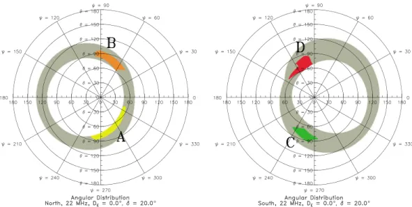
Thus, Figure 4 displays the four high occurrence probability regions in a polar diagram where the direction
𝜓 = 0∘ corresponds to the projection of B over the plane perpendicular to −∇B. This diagram clearly reveals
that for both hemispheres the emission cone is not axisymmetrical around −∇B but is flattened in the direc-tions𝜓 = 0∘ and 𝜓 = 180∘, i.e., in the direction of the local B. It could be thought that this flattening might result from an invisibility of the sources due to a partial exploration of the space (𝜃, 𝜓). In order to prove that it is not the case and that the flattening is quite actual, we have plotted in tan, in Figure 4, all the possible
Figure 4. The four sources Io-A, Io-B, Io-C, and Io-D from Figure 3 are displayed in a polar diagram as a function of the
colatitude angle𝜃(radial coordinate) and the azimuth angle𝜓for both hemispheres. The frequency isf = 22MHz, and the lead angle is𝛿 = 20∘. Such diagrams reveal the beaming cone of the radio emission. In both hemispheres, we note that this cone is not axisymmetrical around−∇Bbut presents a flattening in the direction of the magnetic fieldB. The angular regions explored by the full CML-Io phase diagram are display in tan.
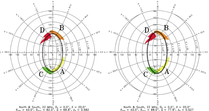
Figure 5. Polar diagram displaying the angular distribution of the four sources Io-A, Io-B, Io-C, and Io-D from Figures 3
and 4 as a function of the colatitude angle𝜃and azimuth angle𝜓. The frequency isf= 22 MHz, the lead angle is
𝛿 = 20∘, and the declination of the Earth is0∘. The green circle at𝜃 = 90∘represents the limit beyond which the propagation is no longer possible. The two red ellipses depict an attempt to fit the emission beam within a hollow cone flattened in the direction of the local magnetic field.
values for (𝜃, 𝜓) derived from the CML-Io phase diagram when 𝜆CMLand ΦIovary from 0∘ to 360∘. Thus, we note that the four sources Io-A, Io-B, Io-C, and Io-D are surrounded by explored zones of the CML-Io phase diagram. Because of this angular layout of the sources, we have been tempted to propose an oblate emission cone with an elliptic section perpendicular to the axis. A fit in the polar diagram of the four sources by ellipses is shown in Figure 5. The transition from a circular section to an elliptic section for the emission cones justifies the use of elliptic coordinates so that each cone can correspond to a fixed value of one of the coordinates. 3.3. Distribution in Elliptic Coordinates
We introduce a system of elliptic coordinates (𝜉, 𝜂) related to the angles (𝜃, 𝜓), described in the previous subsection, by setting the following equations:
𝜃 cos 𝜓 = a sinh 𝜉 cos 𝜂 (12)
𝜃 sin 𝜓 = a cosh 𝜉 sin 𝜂, (13)
where a is a constant scaling factor. Such a coordinate system is shown in Figure 6 where the curves of constant
𝜉 are ellipses while the curves of constant 𝜂 are hyperbolae. All these lines share the same foci, separated by
a distance equal to 2a. Thus, the elliptic beaming cone corresponds to a particular ellipse𝜉 = 𝜉0. It is possible to derive the values of a and𝜉0by considering the minimum (𝜃min) and maximum (𝜃max) opening angles of the flattened emission cone along and perpendicular to the direction of the magnetic field. The quantities a and𝜉0are given by
a = √ 𝜃2 max−𝜃2min (14) 𝜉0=1 2ln [𝜃max +𝜃min 𝜃max−𝜃min ] . (15)
Figure 6. Polar diagram of the distribution of the four sources Io-A, Io-B, Io-C, and Io-D displaying the elliptic coordinate lines which are confocal ellipses
(curves of constant𝜉) and hyperbolae (curves of constant𝜂). The distance between the two foci is2a. For each hemisphere, two numbersaand𝜉0are chosen so that the ellipse𝜉 = 𝜉0fits the source regions. The results are different for the northern sources (left, Io-A, Io-B) and the southern ones (right, Io-C, Io-D): in the northa = 69.8∘and𝜉 = 0.582; in the southa = 77.9∘,𝜉 = 0.527.𝜃min, and𝜃maxcorrespond to the opening angles of the flattened beaming cone in the direction of the magnetic field and the perpendicular direction, respectively. The frequency is stillf= 22 MHz, and the lead angle is𝛿 = 20∘.
The results are found to be different for both Jovian hemispheres. Polar diagram representations of the Io-controlled sources are displayed in Figure 6. Table 2 lists the parameters 𝜃min and𝜃maxcharacterizing the flattened emission cone in both hemispheres and the corresponding values of a and𝜉0derived from equations (14) and (15).
3.4. Oblate Beaming Cone
The introduction of elliptic coordinates (𝜉, 𝜂) allows reconsideration of the contours of the variable opening angle of the emission cone in the CML-Io phase diagram which is expected to be different from the lines of constant𝜃, as in Figure 3. One of the main purposes of our study is to reconcile the location of the four observed sources (Io-A, Io-B, Io-C, and Io-D) with the existence of an active longitude sector.
3.4.1. Confocal Emission Cones and Io-Controlled Sources
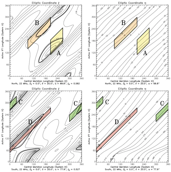
In an analogous manner to what has been done for the angles (𝜃, 𝜓), we have plotted in Figure 7 the contours of the elliptic coordinates𝜉 and 𝜂 for each hemisphere, using the values of a and 𝜉0given in Table 2, as a function of the CML and active magnetic field line longitude. The comparison with Figure 3 is here essential since, in the case of an axisymmetrical emission cone (Figure 3), the contours of𝜃 are open lines which cross the diagram from end to end, whereas in the case of the flattened emission cone (Figure 7) the contour𝜉 = 𝜉0 is a closed line which covers in part the observed source zones. Such a feature is required for the definition of an active longitude sector as described further in subsection 3.5. We also note that the northern and southern emission cones which fit the sources best are slightly different (see the values in Table 2).
Concerning the coordinate𝜂, which characterizes the azimuthal direction around −∇B for the flattened cone, the contours plotted in Figure 7 are very similar to those of𝜓 plotted in Figure 3. This situation is normal since
Table 2. Opening Angles of the Flattened Emission Cone and Corresponding Values ofaand𝜉0
Hemisphere 𝜃min 𝜃max a 𝜉0
North 43∘ 82∘ 69.8∘ 0.582
Figure 7. Contours of the elliptic coordinates (left column)𝜉and (right column)𝜂as a function of the central meridian longitude (System III) and the longitude of the active Io flux tube for the Northern and Southern Hemispheres. The frequency isf= 22 MHz, and the lead angle is𝛿 = 20∘. The regions of high occurrence probability for Io-A, Io-B, Io-C, and Io-D are also displayed. The curves𝜉 = 𝜉0correspond to the trace of the flattened beaming cone derived from Figure 6. The values ofaand𝜉0are distinct for the two hemispheres.
the values of𝜓 and 𝜂 are very close to each other. Indeed, it can be shown from equations (12) and (13) that
𝜂 ≃ 𝜓 − a2
4𝜃2sin 2𝜓. (16)
The mathematical expressions of𝜉(𝜃, 𝜓) and 𝜂(𝜃, 𝜓) are given in Appendix A, together with power series expansions.
3.4.2. Three-Dimensional Representation
The parametric equations describing the emission cone, in the cartesian coordinate system defined by (e1, e2, e3), can be easily derived from equations (12) and (13):
x = sin [ a √ cosh2𝜉0− cos2𝜂 ] sinh𝜉0cos𝜂 √ cosh2𝜉0− cos2𝜂 (17)
Figure 8. Three-dimensional plots of the northern flattened beaming cone derived from our study. Thezaxis is parallel to−∇Bwhile thexaxis is in the direction ofB. The opening angle of the flattened cone is𝜃min= 43∘in the direction of the magnetic field and𝜃max= 82∘in the perpendicular direction (yaxis).
y = sin [ a √ cosh2𝜉0− cos2𝜂 ] cosh𝜉0sin𝜂 √ cosh2𝜉0− cos2𝜂 (18) z = cos [ a √ cosh2𝜉0− cos2𝜂 ] , (19)
with𝜂 varying from 0∘ to 360∘. Figure 8 displays an example of a three-dimensional graphic of the flattened beaming cone derived from our analysis for the Northern Hemisphere. The x and z axes are, respectively, in the direction of the magnetic field B and parallel to its gradient ∇B. The four panels clearly show the variable opening angle of the hollow cone which varies from𝜃min= 43∘ to𝜃max= 82∘.
3.5. Existence of Active Longitude Sector
The highest occurrence probability of the Jovian radio emission is reached when the beaming cone (described by the curve𝜉 = 𝜉0) intersects a longitude range where the emission mechanism (supposed to be the cyclotron maser instability) is the most efficient. In this framework, we have investigated whether it was possible to select a domain of Jovian active longitude𝜆awhich would allow us to recover the source areas
of the CML-Io phase diagram. The result is presented in Figure 9. In Figure 9 (left column), the contours of the coordinate𝜉 have been plotted versus the CML and active IFT longitude, in particular, the line 𝜉 = 𝜉0 which corresponds to the flattened beaming cone. The domain of active longitude, where the amplification is expected to be maximum, is displayed in dark color. The intersection of the emission cone with the active longitude domain is plotted in yellow in Figure 9 (left column) and in red in Figure 9 (right column), where the source zones defined in Table 1 have been displayed in the CML-Io phase diagram. The best fit has been obtained for the following choice of the active domain: 150∘≤ 𝜆a ≤ 270∘ for the Northern Hemisphere and
Figure 9. (left column) Contours of the elliptic coordinate𝜉as a function of the central meridian longitude (System III) and the longitude of the active Io flux tube for the Northern and Southern Hemispheres. A range of active longitude (displayed in dark color) has been chosen in order that the intersection (in yellow) with the flattened beaming cone (𝜉 = 𝜉0) corresponds to the regions of high occurrence probability. The best fit is obtained for 150∘≤ 𝜆a≤ 270∘and 120∘≤ 𝜆a≤ 300∘in the Northern and Southern Hemispheres, respectively. (right column) The intersection of the active longitude domain with the flattened beaming cone is displayed versus central meridian longitude and Io phase (red curves). The regions of high occurrence probability for Io-A, Io-B, Io-C, and Io-D are also displayed. The frequency isf= 22 MHz, and the lead angle is𝛿 = 20∘.
4. Discussion
A long-term ground-based and space observations (of more than a half century) revealed the dependence of the Jovian decametric occurrence probability on specific CMLs. Theoretical investigations [Galopeau et al., 2004, 2007a; Galopeau and Boudjada, 2010] have been devoted to the understanding of the confinement of the Io-controlled emissions at some specific longitude ranges. In our analysis we show that the concept of symmetrical hollow cone, as introduced by Dulk [1965], may only provide an incomplete representation of the emission beam pattern. A hollow cone with an elliptical section is found to fit much more precisely the occurrence area zones of the Io-controlled emissions. In the following, we first discuss the main results of our investigations: the flattening of the emission cone. Afterward, we attempt to examine the classic concept of axisymmetrical amplification in the frame of the maser cyclotron instability. Also, we reconsider the geomet-rical aspects of the hollow cone in the case of the auroral kilometric radiation (AKR) and Saturnian kilometric radiation (SKR). Finally, we wonder about the role of the magnetic field gradient.
4.1. Dissymmetry in CML-Io Phase Diagram
The occurrence diagram of the Io-controlled decameter emission (versus CML and Io phase) is situated in a very particular geometrical context where the radiation emitted in a hollow cone is observed from the plane of the Earth’s orbit. A symmetrical concept has been introduced where Io-A and Io-B on the one hand, and Io-C and Io-D on the other hand are linked to opposite edges of a same hollow cone located in the Northern and Southern Hemispheres, respectively. Hence, from a spectral point of view, one of the edges roughly cor-responds to a vertex early arc structure (e.g., Io-B), whereas the other edge is associated to vertex late arcs (e.g., Io-A). This symmetrical aspect may be noticed in the occurrence areas of Io-A and Io-B or of Io-C and Io-D, which are quiet comparable in the CML-Io phase diagram. However, the area extensions in longitude (CML) are quite different. The CML ranges for Io-A and Io-B occurrence zones are ∼60∘ and ∼120∘, respectively. And a similar disparity between Io-C and Io-D areas is found correspondingly about ∼90∘ and ∼180∘. Several studies attributed those disparities of the occurrence areas to a combined effect of several factors like the observation conditions (e.g., ionospheric conditions and observation frequency), the Earth’s Jovicentric declination, and the emission cone [see e.g., Aubier et al., 2000]. There is no doubt that the flattening of the emission cone, as shown in this paper, is another parameter which also contributes to those discrepan-cies. It is important to note that the observations from space or ground-based stations did not provide a complete coverage of the Jovian DAM emissions in latitude and longitude. The phenomenological aspects (in particular, long-term observations) lead us to bring out on the one hand the presence of an active longi-tude and on the other hand the flattening of the beaming cone. A morphological approach (i.e., a case study of some events) may not allow a full understanding of specific features of the generation mechanism and the build of the emission beam when the radio wave escapes from the source region.
4.2. Amplification and Emergence Angle
Several papers have been devoted to the investigation of the cyclotron maser instability [Wu and Lee, 1979]. The concept of hollow cone was introduced to represent the geometrical emission beam of the Jovian deca-metric radiation when it propagates out of the source region. The cyclotron maser instability (CMI) theory provides a detailed description [Wu, 1985] of the way the mechanism operates. The key physical parameters in this wave-particle interaction are the ratio plasma frequency over gyrofrequency, the parallel and perpen-dicular gradients of electron velocity relative to the ambient magnetic field, and the relativistic Doppler effect in the resonance condition. This theory has been compared to the observations (i.e., the auroral kilometric radiation), it involves particular classes of electron distribution functions in speed, pitch angle, and energy which were identified experimentally. Despite this agreement between the theory and the observations, few investigations have been devoted to study the emission beam pattern of the radio wave. It is a known fact that the CMI theory rests on an emission confined to the surface of a thin hollow cone and at angles of ∼90∘. The axis of symmetry of this hollow cone is tangent to the planetary magnetic field. This symmetry of the cone around the magnetic field line has been usually assumed to be correct. However, investigations have attempted to derive from the CMI theory the geometrical aspects of the emission beam of the radio wave when it propagates out of the source region. Hewitt et al. [1981, 1982] showed that the growth rate maximizes at an angle𝜃 = 𝜃max(where𝜃 is here the angle between the wave vector k and the ambient magnetic field) and falls off rapidly with increasing|𝜃 − 𝜃max|. The authors considered the angle 𝜃maxas the half-angle of the resulting emission cone only if refraction is neglected. Later on, Ladreiter [1991] derived simple expressions relating the wave-emergent angle𝜃 of the amplified wave and the ratio between the plasma frequency and the gyrofrequency (fp∕fc < 0.01). He found an emergent angle at the source of ∼80∘, less than the 90∘ pre-dicted in CMI theory. Melrose and Dulk [1993] attempted to explain the observation of elliptically polarized bursts of the Jovian decametric radio emission: the authors suggested an emission at oblique angle, less than 65∘, where a “spiraling beam distribution” in the velocity space may be considered. Those previous theoretical investigations showed that some factors (refraction effect, particular ratio fp∕fc, or specific speed distribution)
favor different emergent angles which are not usually symmetrical and may be more extended in longitude or latitude.
4.3. Comparison With Terrestrial and Saturnian Radiations
The auroral kilometric radiation (AKR) is considered to be generated, like the Jovian DAM emission, by the CMI mechanism. However, the AKR phenomenological aspect is not well known because of the absence of long-term and regular observations. Despite this characteristic, the artificial satellites around the Earth have provided a clearer picture of the physical conditions (locally and surroundings) when their orbits crossed the source region. The so-called “cavity” has been considered as a geometrical representation of the
AKR source region. Since Viking observations, several investigations showed that the AKR emission beam has a particular geometry with regard to the Earth’s magnetic field. Hence, Louarn and Le Quéau [1996] showed that the radiating diagram likely does not have a cylindrical symmetry with respect to the geomagnetic field. They found that this diagram is anisotropic in a plane perpendicular to the magnetic field. Burinskaya
and Rauch [2007] rediscussed the previous investigations and applied numerical solutions to the dispersion
relation. The authors concluded that the instability growth rate increases with wave vector component directed along a tangent to the source boundary in a plane perpendicular to the magnetic field. In general case, the electromagnetic field in the source has an asymmetrical structure, the ratio of the electric field com-ponents in the source depends on the coordinates, and the electric field component transverse to the source boundary can substantially exceed the component parallel to the boundary. The Cluster constellation satel-lites allowed, applying the very long baseline interferometer (VLBI) technique, analysis of the spatial and temporal properties of AKR bursts [Mutel et al., 2004]. The authors found that distinct auroral kilometric radi-ation bursts are emitted in a narrow plane surface containing the local magnetic field vector and tangent to the magnetic latitude circle at the source. This geometry is in agreement with the longitudinal propagation derived from the numerical models by Louarn and Le Quéau [1996] and Pritchett et al. [2002].
The Saturnian kilometric radiation (SKR) has been usually compared to the Earth’s kilometric emission (AKR) because of the dependence of the source region on local time (dayside for SKR and nightside for AKR), as deduced from Voyager observations [Kaiser and Desch, 1982]. The Cassini mission provided new results con-cerning the radiation directivity which is directly related to the emission beam pattern. However, Cassini investigations also showed the complexity of the interpretation of the SKR observations and the correspond-ing emission beam which crucially depends on the geometrical conditions of the SKR source with regard to the observer. Hence, using radio horizon technique, Farrell et al. [2005] brought out the presence of an emis-sion source associated to the Saturnian kilometric radiation. This source was found to be confined to relatively low latitudes and close to midnight, in discrepancy with Voyager observations which reported a source loca-tion well away from the high-latitude dayside cusp region. Galopeau et al. [2007b] analyzed the spectral shape of the SKR and showed that the radiation may be considered as the overlapping of hollow cones related to three components. The Stokes polarization parameters and the frequency bandwidth were used as criteria to separate those components. Galopeau et al. [2007b, 2009] addressed the problem about the ellipticity of the polarization of the Saturnian radiation, and Fischer et al. [2009] revealed the presence of a strongly elliptically polarized emission when the Cassini spacecraft is at latitudes higher than 30∘.
4.4. Role of Magnetic Field Gradient
Our study does not aim to explain the origin of the flattening of the emission cone as it is revealed by the distri-bution of the occurrence probability in the CML-Io phase diagram. However, an important question remains, what is the role of ∇B in the CMI, which depends on the magnetic field vector B and the angle it makes with respect to the wave vector k? The definition of a local frame linked to a nonuniform magnetic field not only requires the components of the field (Bx, By, Bz) but also their first derivatives (𝜕Bx∕𝜕x, 𝜕Bx∕𝜕y, …) which
constitute a second-order tensor. The simplest situation is that of a frame defined by B and ∇B.
The first calculations devoted to the cyclotron maser instability in an inhomogeneous medium were devel-oped by Le Quéau et al. [1985]: they involved a slow variation of the gyrofrequency in a geometry with axial symmetry where B and ∇B are parallel. The introduction of an inhomogeneity in one dimension tremendously complicates the calculation of the resonance, of the growth rate, and of the emergence angle of the wave. The authors had to consider not only the Wentzel-Kramers-Brillouin approximation for the variation of the waves but also splitting up of the plasma into an energetic and a cold component.
Although in the case of the Jovian decameter emission the medium can be regarded as homogeneous for the CMI (cf. section 2.3) because𝜆DAM ≪ LB = B∕‖∇B‖, the introduction of ∇B attracts one’s attention to
propagation effects (section 3.1). Thus, there is a great temptation to interpret the nonaxisymmetrical cone shape by propagation effects. Nevertheless, two separate domains of propagation shall be distinguished: the propagation inside the radio source, where the amplification by the CMI is occurring, and the (pure) propa-gation outside the source. Besides, a competition between the processes occurring in both domains shall be considered in order to establish possibly which one dominates.
Outside the radio source, the study of the propagation of the radiation is sometimes far from being straight-forward because of the presence of refraction effects at low frequencies. For instance, through a ray tracing
a few megahertz. Moreover, by using a method of physical optics, Lecacheux et al. [1981] showed the existence of a diffraction phenomenon in the Jovian decameter radiation due to the variation of the wave phase during the propagation. Their approach explained many observational features appearing in the dynamic spectra. Inside the radio source, the situation is very different because the propagation contributes to the modification of the growth rate and the emergence angle of the wave when the magnetized plasma is not homogeneous. In a nonaxial symmetry, the mathematical calculation of the growth rate has to be performed.
In our study, the angular representation of the high occurrence zones in polar diagrams (Figures 4–6) causes the loss of all information about their spatial distribution (in particular, in longitude) because of the projection onto the local frame (e1, e2, e3) linked to B and ∇B, so that it is not possible to test propagation effects outside the radio sources. However, the refraction effects revealed by ray tracing methods must not be neglected for the interpretation of the beam pattern, even inside source regions. For instance, using observations of AKR performed by the Polar spacecraft, Menietti et al. [2011] showed that the radiation generated by CMI can be strongly refracted when escaping from low-density cavities. Our results especially suggest to examine both the details of the emission mechanism and the refractive processes in a nonaxial geometry where the vectors
B and ∇B are not parallel.
5. Conclusion
The aim of this paper was the identification of a flattening of the emission cone of the Io-controlled Jovian decameter radiation based on the statistical distribution of the high occurrence regions in the CML-Io phase diagram, which is built from a set of long-term observations. We have obtained very similar results for both Northern and Southern Hemispheres of Jupiter: a hollow cone with an elliptic section, an axis parallel to −∇B, and a flattening in the direction of the magnetic field vector B. This flattening is not negligible because the opening angle of the emission cone varies from𝜃min = 43∘ to𝜃max= 82∘ in the Northern Hemisphere and from𝜃min= 43∘ to𝜃max= 89∘ in the Southern Hemisphere; our study has been done for an emission frequency
f = 22 MHz and a lead angle𝛿 = 20∘ (representing the difference in longitude between the active magnetic
field line and the position of Io).
A major consequence of our result is that the flattening of the emission cone allows the theoretical exis-tence of an active longitude sector (favoring the radiation) much more easily than in the case of a cone having an axial symmetry (i.e., with a constant opening angle). In this context, the zones of maximum theoretical amplification correspond to the regions of high occurrence probability observed in the CML-Io phase diagram.
Abandoning the assumption of a radiation within a hollow cone with axial symmetry becomes relevant not only in the case of the decametric radio emissions of Jupiter but also in the frame of the kilometric radiations of the Earth and Saturn. A further calculation of the cyclotron maser instability in an inhomogeneous and nonaxisymmetrical medium (i.e., in presence of nonparallel vectors ∇B and B) has to be done in order to give a theoretical framework to the role played by the source mechanism in the existence of such an oblate beaming cone.
Appendix A: From Polar to Elliptic Coordinates
In the following, we present some formulae useful for the change from polar coordinates (𝜃, 𝜓) to elliptic coordinates (𝜉, 𝜂) (see section 3); more precisely, we give the expressions of 𝜉(𝜃, 𝜓) and 𝜂(𝜃, 𝜓). We also show power series expansions when the value of𝜃 is small or large.
The equations of the coordinate transformation are
𝜃 cos 𝜓 = a sinh 𝜉 cos 𝜂 (A1)
𝜃 sin 𝜓 = a cosh 𝜉 sin 𝜂. (A2)
Eliminating𝜂 between (A1) and (A2), one gets ( 𝜃 sin𝜓 cosh𝜉 )2 + ( 𝜃cos𝜓 sinh𝜉 )2 = a2 (A3)
and then a2 𝜃2sinh 4𝜉 + ( a2 𝜃2− 1 )
sinh2𝜉 − cos2𝜓 = 0, (A4)
which can be solved as
tanh𝜉 = √ √ √ √ 𝜃2− a2+√a4+ 2a2𝜃2cos 2𝜓 + 𝜃4 𝜃2+ a2+√a4+ 2a2𝜃2cos 2𝜓 + 𝜃4. (A5)
On the other hand, from (A1) and (A2) one derives
tan𝜂 = tanh 𝜉 ⋅ tan 𝜓; (A6)
hence, tan𝜂 = tan 𝜓 ⋅ √ √ √ √ 𝜃2− a2+√a4+ 2a2𝜃2cos 2𝜓 + 𝜃4 𝜃2+ a2+√a4+ 2a2𝜃2cos 2𝜓 + 𝜃4. (A7) Setting K =𝜃4+ 2a2𝜃2cos 2𝜓 + a4, (A8)
one finally obtains from (A5) and (A7)
𝜉 = ln √ 𝜃2− a2+√K + √ 𝜃2+ a2+√K √ 2a (A9) 𝜂 = atan⎛⎜⎜ ⎝ √ √ √ √ 𝜃2− a2+√K 𝜃2+ a2+√K ⋅ tan 𝜓 ⎞ ⎟ ⎟ ⎠ (+𝜋 if cos 𝜓 < 0). (A10)
In case𝜃 ≫ a, a power series expansion for 𝜉(𝜃, 𝜓) and 𝜂(𝜃, 𝜓) with respect to 𝜃 can be derived from equations (A8)– (A10) with the help of Wolfram Mathematica®;:
√
K =𝜃2+ a2cos 2𝜓 + a
4
2𝜃2sin
22𝜓 − a6
4𝜃4sin 2𝜓 sin 4𝜓 + ... (A11)
therefore, 𝜉 = ln2𝜃 a + a2 4𝜃2cos 2𝜓 − 3a4 32𝜃4cos 4𝜓 + … (A12) 𝜂 = 𝜓 − a2 4𝜃2sin 2𝜓 + 3a4 32𝜃4sin 4𝜓 + … (A13)
In case𝜃 ≪ a and cos 𝜓 > 0, a power series expansion for 𝜉 and 𝜂 with respect to 𝜃 can be calculated in the same way: √ K = a2+𝜃2cos 2𝜓 + 𝜃 4 2a2sin 22𝜓 − 𝜃6
4a4sin 2𝜓 sin 4𝜓 + … (A14)
hence, 𝜉 = 𝜃 acos𝜓 − 𝜃 3 6a3cos 3𝜓 + 3𝜃5
40a5cos 5𝜓 + … (A15)
𝜂 = 𝜃
asin𝜓 − 𝜃 3
6a3sin 3𝜓 +
3𝜃5
References
Aubier, A., M. Y. Boudjada, P. Moreau, P. H. M. Galopeau, A. Lecacheux, and H. O. Rucker (2000), Statistical studies of Jovian decameter emissions observed during the same period by Nançay Decameter Array (France) and WAVES experiment aboard Wind spacecraft, Astron. Astrophys., 354, 1101–1109.
Benson, R. F., and W. Calvert (1979), ISIS 1 observations at the source of auroral kilometric radiation, Geophys. Res. Lett., 6, 479–482, doi:10.1029/GL006i006p00479.
Bigg, E. K. (1964), Influence of the satellite Io on Jupiter’s decametric emission, Nature, 203, 1008–1011, doi:10.1038/2031008a0. Boudjada, M. Y., and Y. Leblanc (1992), The variability of Jovian decametric radiation from 1978 to 1988, Adv. Space Res., 12(8), 95–98,
doi:10.1016/0273-1177(92)90382-8.
Burinskaya, T. M., and J. L. Rauch (2007), Waveguide regime of cyclotron maser instability in plasma regions of depressed density, Plasma Phys. Rep., 33, 28–37, doi:10.1134/S1063780X07010047.
Burke, B. F., and K. L. Franklin (1955), Observations of a variable radio source associated with planet Jupiter, J. Geophys. Res., 60(2), 213–217, doi:10.1029/JZ060i002p00213.
Calvert, W. (1981), The signature of auroral kilometric radiation on ISIS 1 ionograms, J. Geophys. Res., 86, 76–82, doi:10.1029/JA086iA01p00076.
Carr, T. D., M. D. Desch, and J. K. Alexander (1983), Phenomenology of magnetospheric radio emissions, in Physics of the Jovian Magnetosphere, edited by A. J. Dessler, pp. 226–284, Cambridge Univ. Press, New York.
Dulk, G. A. (1965), Io-related radio emission from Jupiter, Science, 148, 1585–1589, doi:10.1126/science.148.3677.1585. Ergun, R. E., et al. (1998), FAST satellite wave observations in the AKR source region, Geophys. Res. Lett., 25, 2061–2064,
doi:10.1029/98GL00570.
Farrell, W. M., M. D. Desch, M. L. Kaiser, A. Lecacheux, W. S. Kurth, D. A. Gurnett, B. Cecconi, and P. Zarka (2005), A nightside source of Saturn’s kilometric radiation: Evidence for an inner magnetosphere energy driver, Geophys. Res. Lett., 32, L18107, doi:10.1029/2005GL023449. Fischer, G., B. Cecconi, L. Lamy, S.-Y. Ye, U. Taubenschuss, W. Macher, P. Zarka, W. S. Kurth, and D. A. Gurnett (2009), Elliptical polarization of
Saturn Kilometric Radiation observed from high latitudes, J. Geophys. Res., 114, A08216, doi:10.1029/2009JA014176.
Galopeau, P. H. M., and M. Y. Boudjada (2010), Evidence of Jovian active longitude: 3. Observational constraints, J. Geophys. Res., 115, A12221, doi:10.1029/2010JA015677.
Galopeau, P. H. M., M. Y. Boudjada, and H. O. Rucker (2004), Evidence of Jovian active longitude: 1. Efficiency of cyclotron maser instability, J. Geophys. Res., 109, A12217, doi:10.1029/2004JA010459.
Galopeau, P. H. M., M. Y. Boudjada, and H. O. Rucker (2007a), Evidence of Jovian active longitude: 2. A parametric study, J. Geophys. Res., 112, A04211, doi:10.1029/2006JA011911.
Galopeau, P. H. M., M. Y. Boudjada, and A. Lecacheux (2007b), Spectral features of SKR observed by Cassini/RPWS: Frequency bandwidth, flux density and polarization, J. Geophys. Res., 112, A11213, doi:10.1029/2007JA012573.
Galopeau, P. H. M., M. Y. Boudjada, and A. Lecacheux (2009), Reply to comment by B. Cecconi on “Spectral features of SKR observed by Cassini/RPWS: Frequency bandwidth, flux density and polarization”, J. Geophys. Res., 114, A07207, doi:10.1029/2008JA013177. Genova, F., and M. G. Aubier (1985), Io-dependent sources of the Jovian decameter emission, Astron. Astrophys., 150, 139–150. Goldstein, M. L., and J. R. Thieman (1981), The formation of arcs in the dynamic spectra of Jovian decameter bursts, J. Geophys. Res., 86,
8569–8578, doi:10.1029/JA086iA10p08569.
Green, J. L., D. A. Gurnett, and S. D. Shawhan (1977), The angular distribution of auroral kilometric radiation, J. Geophys. Res., 82, 1825–1838, doi:10.1029/JA082i013p01825.
Hashimoto, K., and M. L. Goldstein (1983), A theory of the Io phase asymmetry of the Jovian decametric radiation, J. Geophys. Res., 88, 2010–2020, doi:10.1029/JA088iA03p02010.
Hewitt, R. G., D. B. Melrose, and K. G. Rönnmark (1981), A cyclotron theory for the beaming pattern of Jupiter’s decametric radio emission, Proc. Astron. Soc. Aust., 4, 221–226.
Hewitt, R. G., D. B. Melrose, and K. G. Rönnmark (1982), The loss-cone driven electron-cyclotron maser, Aust. J. Phys., 35, 447–471. Hilgers, A., A. Roux, and R. Lundin (1991), Characteristics of AKR sources; A statistical description, Geophys. Res. Lett., 18, 1493–1496,
doi:10.1029/91GL01332.
Kaiser, M. L., and M. D. Desch (1982), Saturnian kilometric radiation: Source locations, J. Geophys. Res., 87(A6), 4555–4559, doi:10.1029/JA087iA06p04555.
Kuril’chik, V. N., I. F. Kopaeva, and S. V. Mironov (2006), Observations of the auroral kilometric radiation onboard the Interball-1 satellite in 1995–1997, Cosmic Res., 44, 95–105, doi:10.1134/S001095250602002X.
Ladreiter, H. P. (1991), The cyclotron maser instability: Application to low-density magnetoplasmas, Astrophys. J., 370, 419–426, doi:10.1086/169828.
Leblanc, Y. (1981), On the arc structure of the DAM Jupiter emission, J. Geophys. Res., 86(A10), 8546–8560, doi:10.1029/JA086iA10p08546. Lecacheux, A. (1981), Ray tracing in the Io plasma torus: Application to the PRA observations during Voyager 1’s closest approach,
J. Geophys. Res., 86, 8523–8528, doi:10.1029/JA086iA10p08523.
Lecacheux, A., N. Meyer-Vernet, and G. Daigne (1981), Jupiter’s decametric radio emission: A nice problem of optics, Astron. Astrophys., 94, L9–L12.
Lecacheux, A., A. Boischot, M. Y. Boudjada, and G. A. Dulk (1991), Spectra and complete polarization state of two, Io-related, radio storms from Jupiter, Astron. Astrophys., 251, 339–348.
Lecacheux, A., M. Y. Boudjada, H. O. Rucker, J. L. Bougeret, R. Manning, and M. L. Kaiser (1998), Jovian decameter emissions observed by the Wind/WAVES radioastronomy experiment, Astron. Astrophys., 329, 776–784.
Le Quéau, D., R. Pellat, and A. Roux (1985), The maser synchrotron instability in an inhomogeneous medium: Application to the generation of the auroral kilometric radiation, Ann. Geophys., 3, 273–291.
Louarn, P., and D. Le Quéau (1996), Generation of the Auroral Kilometric Radiation in plasma cavities—I. Experimental study, Planet Space Sci., 44, 199–210, doi:10.1016/0032-0633(95)00121-2.
Melrose, D. B., and G. A. Dulk (1993), Electron cyclotron maser emission at oblique angles, Planet. Space Sci., 41, 333–339, doi:10.1016/0032-0633(93)90066-B.
Menietti, J. D., and D. B. Curran (1990), Instantaneous Io flux tube as the source of Jovian DAM: Possible second harmonic emissions, J. Geophys. Res., 95, 21,273–21,280, doi:10.1029/JA095iA12p21273.
Menietti, J. D., J. L. Green, S. Gulkis, and F. Six (1984a), Three-dimensional ray tracing of the Jovian magnetosphere in the low-frequency range, J. Geophys. Res., 89, 1489–1495, doi:10.1029/JA089iA03p01489.
Menietti, J. D., J. L. Green, S. Gulkis, and N. F. Six (1984b), Jovian decametric arcs: An estimate of the required wave normal angles from three-dimensional ray tracing, J. Geophys. Res., 89, 9089–9094, doi:10.1029/JA089iA10p09089.
Acknowledgments
The study presented in this paper is based on results and conclusions already published in many papers which we have cited in the References. There is no new data in this study.
Menietti, J. D., R. L. Mutel, I. W. Christopher, K. A. Hutchinson, and J. B. Sigwarth (2011), Simultaneous radio and optical observations of auroral structures: Implications for AKR beaming, J. Geophys. Res., 116, A12219, doi:10.1029/2011JA017168.
Mutel, R., D. Gurnett, and I. Christopher (2004), Spatial and temporal properties of AKR burst emission derived from Cluster WBD VLBI studies, Ann. Geophys., 22, 2625–2632, doi:10.5194/angeo-22-2625-2004.
Mutel, R. L., I. W. Christopher, and J. S. Pickett (2008), Cluster multispacecraft determination of AKR angular beaming, Geophys. Res. Lett., 35, L07104, doi:10.1029/2008GL033377.
Pearce, J. B. (1981), A heuristic model for Jovian decametric arcs, J. Geophys. Res., 86, 8579–8580, doi:10.1029/JA086iA10p08579. Pritchett, P. L., R. J. Strangeway, R. E. Ergun, and C. W. Carlson (2002), Generation and propagation of cyclotron maser emissions in the finite
auroral kilometric radiation source cavity, J. Geophys. Res., 107(A12), 1437, doi:10.1029/2002JA009403.
Thieman, J. R., and A. G. Smith (1979), Detailed geometrical modeling of Jupiter’s Io-related decametric radiation, J. Geophys. Res., 84(A6), 2666–2674, doi:10.1029/JA084iA06p02666.
Wilkinson, M. H. (1989), Io-related Jovian decametric arcs, J. Geophys. Res., 94, 11,777–11,790, doi:10.1029/JA094iA09p11777. Wu, C. S. (1985), Kinetic cyclotron and synchrotron maser instabilities: Radio emission processes by direct amplification of radiation,
Space Sci. Rev., 41, 215–298, doi:10.1007/BF00190653.
Wu, C. S., and L. C. Lee (1979), A theory of the terrestrial kilometric radiation, Astrophys. J., 230, 621–626, doi:10.1086/157120.
Zaitsev, V. V., V. E. Shaposhnikov, and H. O. Rucker (2006), Dependence of the Io-related decametric radio emission of Jupiter on the central meridian longitude and Io’s “active” longitudes, Astron. Astrophys., 454, 669–676, doi:10.1051/0004-6361:20054450.