HAL Id: hal-00296037
https://hal.archives-ouvertes.fr/hal-00296037
Submitted on 27 Sep 2006
HAL is a multi-disciplinary open access
archive for the deposit and dissemination of
sci-entific research documents, whether they are
pub-lished or not. The documents may come from
teaching and research institutions in France or
abroad, or from public or private research centers.
L’archive ouverte pluridisciplinaire HAL, est
destinée au dépôt et à la diffusion de documents
scientifiques de niveau recherche, publiés ou non,
émanant des établissements d’enseignement et de
recherche français ou étrangers, des laboratoires
publics ou privés.
used in the Warner and McIntyre gravity wave
parameterization scheme
M. Ern, P. Preusse, C. D. Warner
To cite this version:
M. Ern, P. Preusse, C. D. Warner. Some experimental constraints for spectral parameters used in the
Warner and McIntyre gravity wave parameterization scheme. Atmospheric Chemistry and Physics,
European Geosciences Union, 2006, 6 (12), pp.4361-4381. �hal-00296037�
© Author(s) 2006. This work is licensed under a Creative Commons License.
Chemistry
and Physics
Some experimental constraints for spectral parameters used in the
Warner and McIntyre gravity wave parameterization scheme
M. Ern1, P. Preusse1, and C. D. Warner2
1Institute for Stratospheric Research (ICG-I), Forschungszentrum Juelich, Juelich, Germany 2Centre for Atmospheric Science, University of Cambridge, Cambridge, UK
Received: 8 March 2006 – Published in Atmos. Chem. Phys. Discuss.: 14 June 2006
Revised: 1 September 2006 – Accepted: 17 September 2006 – Published: 27 September 2006
Abstract. In order to incorporate the effect of gravity waves
(GWs) on the atmospheric circulation most global circula-tion models (GCMs) employ gravity wave parameterizacircula-tion schemes. To date, GW parameterization schemes in GCMs are used without experimental validation of the set of global parameters assumed for the GW launch spectrum. This pa-per focuses on the Warner and McIntyre GW parameteriza-tion scheme. Ranges of parameters compatible with abso-lute values of gravity wave momentum flux (GW-MF) de-rived from CRISTA-1 and CRISTA-2 satellite measurements are deduced for several of the parameters and the limitations of both model and measurements are discussed. The find-ings presented in this paper show that the initial guess of spectral parameters provided by Warner and McIntyre (2001) are some kind of compromise with respect to agreement of absolute values and agreement of the horizontal structures found in both measurements and model results. Better agree-ment can be achieved by using a vertical wavenumber launch spectrum with a wider saturated spectral range and reduced spectral power in the unsaturated part. However, even with this optimized set of global launch parameters not all fea-tures of the measurements are matched. This indicates that for further improvement spatial and seasonal variations of the launch parameters should be included in GW parameteriza-tion schemes.
1 Introduction
Gravity waves (GWs) are one of the most important vertical coupling processes in the atmosphere transferring momen-tum from the troposphere into the stratosphere and meso-sphere and contributing to the acceleration and decelera-tion of the horizontal wind. A review of GW dynamics
Correspondence to: M. Ern
has been given by Fritts and Alexander (2003). Since the spatial resolution in global circulation models (GCMs) is not sufficient to resolve medium scale processes like grav-ity waves the contribution of GWs to the model dynamics is calculated with GW parameterization schemes. Different ap-proaches have led to a number of different parameterization schemes (e.g., Lindzen, 1981; McFarlane, 1987; Medvedev and Klaassen, 1995; Hines, 1997a,b; Warner and McIntyre, 2001) with spectral parameterizations being the latest devel-opment. A review about GW parameterization schemes is given by Kim et al. (2003).
Parameterizing instead of resolving GW processes in a GCM allows the use of model grids with lower spatial reso-lution and reduces the computational cost dramatically, a re-quirement which is important especially for long-term model runs. In spectral GW parameterization schemes a GW spec-tral distribution (launch spectrum) is launched at a fixed al-titude (launch alal-titude). Then the wave spectrum is propa-gated vertically through the background atmosphere. There are several parameters that are more or less freely adjustable. One parameter is the launch altitude itself. Other parameters define the spectral shape of the GW spectrum at the launch altitude.
There are some assumptions about the properties of the GW spectrum which are commonly made. Supported by var-ious observations (e.g., Sato, 1994; Nastrom et al., 1997; Cot, 2001; Hertzog and Vial, 2001; Hertzog et al., 2001, 2002; Tsuda et al., 2004) the intrinsic frequency ˆωspectrum of the GW total wave energy density often is assumed to decrease with ˆω−pfor large values of ˆωand typically a value of p=5/3 is used.
Also well-constrained is the vertical wavenumber m spec-trum in its saturated part at large vertical wavenumbers m: there are numerous observations that the saturated part of the vertical wavenumber spectrum obeys a power law ∼m−t and decreases with a power of t≈3 (e.g., VanZandt, 1982; Tsuda et al., 1989, 1991; Sato, 1993, 1994; Allen and
Vin-vertical wavenumber m
GW momentum flux spectral density
part 1 part 2
m*
~ms
~m-t
Fig. 1. GW momentum flux vertical wavenumber spectrum used
in the Warner and McIntyre GW scheme at the model launch level. The spectrum consists of two parts: the unsaturated part (part 1,
m<m∗) is ∼ms, the saturated part (part 2, m>m∗) is ∼m−t.
cent, 1995; Hertzog et al., 2001). On the other hand, the un-saturated part of the vertical wavenumber spectrum (at small vertical wavenumbers m) is not well defined observationally or theoretically (Fritts and Alexander, 2003).
For the characteristic wavenumber m* separating the sat-urated from the unsatsat-urated part of the vertical wavenum-ber spectrum typical values of about 0.2–0.5 cycles/km have been reported for the lower stratosphere (Allen and Vin-cent, 1995; Hertzog et al., 2001; Tsuda and Hocke, 2002). However, the values given are subject to larger uncertainties mainly due to the required detrending of the vertical profiles of observations. In addition, the meteorological conditions at the measurement locations play an important role.
All these assumptions and observations are incorporated in the GW parameterization schemes used in GCMs. In the Warner and McIntyre GW parameterization scheme (Warner and McIntyre, 1996, 1999, 2001) for simplification the verti-cal wavenumber (m) launch spectrum for gravity wave mo-mentum flux (GW-MF) is divided into two parts: The un-saturated part at low vertical wavenumbers m is assumed to increase with ms (with a small-m cutoff value m
cut). In
Warner and McIntyre (2001) a standard value of s=1 is used. However, this spectral slope is not very well defined by ob-servations or theoretically (Fritts and Alexander, 2003). The saturated part of the spectrum at high vertical wavenumbers is assumed to decline with m−t with the standard value t=3. The characteristic wavenumber m* separates the unsaturated from the saturated spectral part (see Fig. 1).
Another parameter β defines the value of the GW energy density E0at the launch level:
E0=βN2/m∗2 (1)
where N is the buoyancy frequency. In the Warner and McIn-tyre scheme the value of β is proportional to the amount of GW-MF (at all altitudes) and the GW drag derived from it. From theoretical assumptions the value of β is about 0.1 with an uncertainty of about a factor of two (Warner and McIn-tyre, 1996; Fritts and Alexander, 2003). Since β in the way it is used in the Warner and McIntyre GW parameterization scheme simply scales the values of GW-MF and gravity wave drag without changing relative structures of the overall distri-butions this value of β will be used for all calculations shown in this manuscript (see Sects. 3, 4 and 5).
The choice of these launch parameters is based more on theoretical assumptions than on observations (Warner and McIntyre, 1996, 1999, 2001). This is why normally fixed parameter values are taken for all longitudes and latitudes, and global variations of these values due to different sources and mechanisms exciting GWs remain out of consideration. This means the Warner and McIntyre GW scheme (like all other general GW parameterization schemes) will describe only the global background distribution of GWs.
In particular, orographically excited GWs (mountain waves) and GWs excited by deep convection, mainly in the tropics and subtropics, are not covered by these general GW parameterization schemes. GWs excited by those processes have to be described by separate models (McFarlane, 1987; Eckermann et al., 2000; Chun and Baik, 1998, 2002; Beres et al., 2005).
Global data sets of observed GW-MF can help to remedy the lack of experimental constraints. It can be tested whether the simplifying assumptions mentioned above are justified and, in particular, whether a GW parameterization scheme with a selected set of fixed model parameters is able to re-produce the observed horizontal and vertical patterns of GW-MF.
This comparison has to be made in terms of momentum flux rather than comparing potential wave energy. The scale separation approach (cf. Sect. 3 and Appendix A) to isolate GWs from other atmospheric fluctuations retains also iner-tio GWs of very long horizontal wavelengths. These waves predominately exist at the equator (Alexander et al., 2002), but can spread to higher latitudes with increasing altitudes (Preusse et al., 2006) propagating several 1000 km in the horizontal. These waves cannot be described by a model assuming mid frequency approximation and purely vertical wave propagation. Though these waves are contributing a large part of the measured wave potential energy they con-tribute little to the measured momentum flux (Ern et al., 2004; Preusse et al., 2006) and they are badly represented in the parameterization scheme. Comparing momentum flux, hence makes model and measurement comparable at all and, in addition, strengthens the scale separation approach by fo-cusing on shorter horizontal wavelengths less likely influ-enced by non-GW signatures (cf. Appendix A).
The only true global experimental data set of GW-MF available was derived from temperature altitude profiles
measured by the CRyogenic Infrared Spectrometers and Telescopes for the Atmosphere (CRISTA) instrument (Ern et al., 2004). Therefore the purpose of this paper is to com-pare GW-MF distributions from both CRISTA flights with simulated distributions from the Warner and McIntyre GW parameterization scheme and by variation of the free param-eters to infer constraints for the model launch paramparam-eters.
2 CRISTA gravity wave momentum flux
2.1 Algorithm
The CRISTA instrument was part of two Space Shuttle missions in November 1994 (CRISTA-1) and August 1997 (CRISTA-2). A high-resolution measuring grid in all three spatial dimensions was obtained by using three telescopes simultaneously and by cooling the instrument with supercrit-ical helium to improve the measurement speed (Offermann et al., 1999). Atmospheric temperatures were derived from CO2infrared limb emissions at 12.6 µm (Riese et al., 1999).
To separate temperature fluctuations due to GWs from larger scale atmospheric structures like planetary waves, the temperature data were detrended using a zonal wavenumber 0–6 Kalman filter. The so-obtained vertical profiles of resid-ual temperatures were analyzed for GWs using a combina-tion of maximum entropy method and harmonic analysis and vertical profiles of GW amplitudes, vertical wavelengths and phases of the two strongest vertical wave components were derived (Preusse et al., 2002).
The short horizontal sampling distance of about 200 km along the satellite track is just sufficient to estimate the hor-izontal wavelengths of the GWs from GW phase differences between pairs of consecutive altitude profiles. Based on the determined GW temperature amplitudes, vertical and hori-zontal wavelengths it was possible to derive absolute values of GW-MF from satellite data for the first time (Ern et al., 2004).
Only absolute values of GW-MF (i.e., not the direction of GW-MF) could be derived due to limitations of the horizontal sampling. To derive vectors of GW-MF a high-resolution 2-D horizontal sampling of about 40 km along and about 40 km across the satellite track is needed (Riese et al., 2005).
Another problem when determining GW-MF are aliasing effects: The limb scanning geometry allows CRISTA to de-tect GWs with horizontal wavelengths as short as ∼100 km (Preusse et al., 2002; Ern et al., 2005). This is much shorter than the limiting wavelength (Nyquist wavelength) of 400 km (i.e. twice the horizontal sampling distance along the satellite track) that can be resolved unambiguously by the CRISTA horizontal sampling. Therefore limitations arising from the CRISTA sampling are more severe than those arising from the limb scanning geometry.
This undersampling of GWs causes aliasing effects: hori-zontal wavelengths determined for the fraction of
undersam-pled waves are systematically too long and the GW-MF car-ried by these waves is underestimated. To compensate for this low-bias in CRISTA GW-MF an aliasing correction has been applied. Of course, such an empirical correction is sub-ject to large errors. The correction is based on the mean hor-izontal wavelength in regions of 30◦longitude times 20◦ lat-itude (Ern et al., 2004) and generally increases the CRISTA GW-MF values. The average correction is about a factor of 1.7 and the correction is limited to not more than a factor of 2. Largest corrections are made at high northern and high southern latitudes. Hence, the contrast between equatorial and polar latitudes is enhanced. For a more detailed descrip-tion of the GW-MF algorithm see Ern et al. (2004).
The single-wave spectral results from CRISTA altitude profiles will be compared with results from a spectral GW parameterization. Since a spectral model reflects the GW mean state at a given location we have to average over the single CRISTA profiles to obtain comparable values. There-fore for all further analyses the GW-MF values determined for the abovementioned regions of 30◦longitude times 20◦ latitude will be used. Averaging the CRISTA profiles has also the advantage of reducing the scatter due to intermittent GW sources inherent in the single CRISTA profiles. In addi-tion, aliasing corrected GW-MF values can be used.
2.2 GW-MF during CRISTA-1 and CRISTA-2
There are some differences between the CRISTA-1 (Novem-ber 1994) and CRISTA-2 (August 1997) data sets with re-spect to GW analysis, derivation of GW-MF, and the inter-pretation of the results.
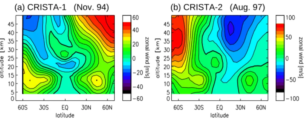
First, the meteorological conditions during the two CRISTA missions were different. Latitude altitude cross sec-tions of the zonal mean zonal wind for the CRISTA-1 and CRISTA-2 missions are shown in Fig. 2. During CRISTA-2 there is a wind reversal in the northern hemisphere already at low altitudes between 20 and 25 km (see Fig. 2b).
This wind reversal prevents mountain waves from propa-gating towards higher altitudes. In the southern hemisphere there is no wind reversal and mountain waves can propa-gate through the whole stratosphere. However, there are only few major mountain ridges in the southern hemisphere. Therefore orographic GWs should not be a dominant effect. Since nonorographic GW parameterization schemes (e.g., the Warner and McIntyre GW parameterization scheme) do not cover contributions due to mountain waves the CRISTA-2 data set of GW-MF should be suited better for compar-isons with those models than, for example, the CRISTA-1 GW-MF data. During CRISTA-1 there is no wind reversal in the northern hemisphere and the wind reversal observed in the southern hemisphere is at higher altitudes (about 20– 35 km depending on latitude, see Fig. 2a). Therefore part of the GWs observed during CRISTA-1 are mountain waves (see also Eckermann and Preusse, 1999; Preusse et al., 2002; Jiang et al., 2004a).
(b) CRISTA-2 (Aug. 97)
zonal wind [m/s]
(a) CRISTA-1 (Nov. 94)
zonal wind [m/s]
Fig. 2. Zonal mean zonal wind for CRISTA-1 (a) and CRISTA-2 (b) calculated from UKMO data interpolated to CRISTA measurement
times and locations. Zero wind is represented by a bold contour line. Please note that the color code is different in (a) and (b).
In addition, the CRISTA-2 GW-MF data should generally be better suited for global comparisons due to the observed strong meridional variation of GW-MF with very high values in the region of the southern polar jet (Ern et al., 2004), pro-viding a high-contrast distribution of GW-MF. This merid-ional variation is less pronounced in the CRISTA-1 GW-MF data, see also Sect. 3. Due to differences between the mea-surement modes of the two CRISTA missions the CRISTA-2 values of GW-MF also cover a larger altitude interval (about 20–50 km) compared to CRISTA-1 (about 20–40 km).
3 Horizontal distributions of CRISTA GW-MF com-pared to standard Warner and McIntyre scheme re-sults
Previous investigations have shown that good agreement be-tween the GW-MF horizontal distributions at 25 km alti-tude obtained from CRISTA-2 and the Warner and McIntyre scheme using the standard set of launch parameters (s=1,
λ∗z,launch=2π/m∗
launch=2 km) can only be achieved if a low
model GW launch level is chosen (Ern et al., 2004, 2005). It should be mentioned that we always use the standard value
β≈0.1 without loss of generality since β in the Warner and McIntyre GW parameterization scheme simply scales the GW-MF values without changing the relative distributions (see Sect. 1).
Using higher launch levels usually results in model GW-MF distributions too symmetric with respect to the equator and the longitudinal structure of GW-MF is not reproduced properly (Ern et al., 2004, 2005). In this section some exam-ples are shown for both CRISTA-1 and CRISTA-2 and a low model launch level of 464 mbar (about 5.4 km).
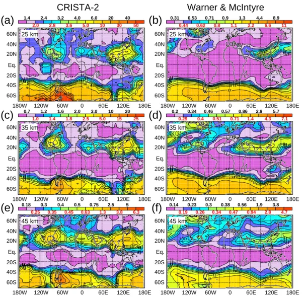
Figure 3 shows horizontal distributions of GW-MF abso-lute values for CRISTA-2 at altitudes of 25 km (Fig. 3a), 35 km (Fig. 3c), and 45 km (Fig. 3e). Also shown are re-sults of GW-MF absolute values calculated with the Warner and McIntyre GW parameterization scheme using meteoro-logical data (temperature and wind fields) from the UK Met
Office (UKMO) stratosphere-troposphere assimilation sys-tem (Swinbank and O’Neill, 1994) interpolated to CRISTA-2 measurement times and locations for the same altitudes (25 km (Fig. 3b), 35 km (Fig. 3d), and 45 km (Fig. 3f)). The model GW-MF results are filtered according to the horizon-tal and vertical wavelengths of GWs visible for the CRISTA instrument: CRISTA is able to detect waves with horizontal wavelengths from ∼100 km to ∼5000 km and vertical wave-lengths in the intervals λz ∈ [5 km, 25 km] (CRISTA-1) and
λz∈ [6 km, 30 km] (CRISTA-2) (Ern et al., 2005).
Obviously, the good agreement between the horizontal rel-ative structures of both CRISTA-2 and model data found ear-lier by Ern et al. (2004) at 25 km altitude is also valid for the other altitudes. There are some differences in details of the horizontal structures. For example, the very high values of GW-MF found in the CRISTA-2 data over the Antarctic Peninsula and the southern tip of South America, or the high values over Southeast Asia and the Gulf of Mexico, are all underrepresented in the model results and indicate localized GW sources in these regions. On the other hand, there is slightly too much GW-MF in the northernmost latitudes of the model results, especially at 45 km altitude. It should also be mentioned that the color scales of Figs. 3a–f are all differ-ent to allow the comparison of horizontal structures (see con-tour labels). At 25 km altitude the model values of GW-MF are considerably lower than the CRISTA-2 values by over a factor of 5 (global average), whereas at 45 km altitude the model values are lower than the CRISTA-2 values by not more than a factor of about 2 (global average).
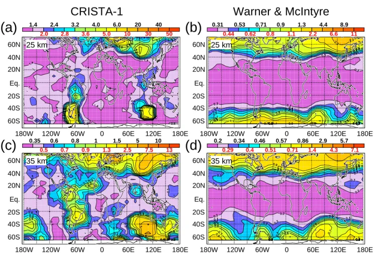
Figure 4 shows a comparison between CRISTA-1 GW-MF absolute values and Warner and McIntyre results like the one in Fig. 3 with the same model launch parameters (launch level 464 mbar, s=1, and λ∗z,launch=2 km). Since the altitude range of the CRISTA-1 GW-MF data is smaller only altitudes of 25 km and 35 km are shown for the CRISTA-1 (Figs. 4a, c) and the model data (Figs. 4b, d). Again, the color scales are different in Figs. 4a–d to highlight features of the horizontal distributions.
60N 40N 20N Eq. 20S 40S 60S
180W 120W 60W 0 60E 120E 180E 60N 40N 20N Eq. 20S 40S 60S
180W 120W 60W 0 60E 120E 180E
60N 40N 20N Eq. 20S 40S 60S
180W 120W 60W 0 60E 120E 180E 60N 40N 20N Eq. 20S 40S 60S
180W 120W 60W 0 60E 120E 180E
60N 40N 20N Eq. 20S 40S 60S
180W 120W 60W 0 60E 120E 180E 60N 40N 20N Eq. 20S 40S 60S
180W 120W 60W 0 60E 120E 180E
(a)
(b)
(d)
(f)
(c)
(e)
CRISTA-2
Warner & McIntyre
25 km 25 km 35 km 45 km 45 km 35 km 1.4 2.0 2.4 2.8 3.2 3.6 4.0 5.0 6.0 10 20 30 40 50 0.7 1.0 1.2 1.4 1.6 1.8 2.0 2.5 3.0 5.0 10 15 20 25 0.2 0.29 0.34 0.4 0.46 0.51 0.57 0.71 0.86 1.4 2.9 4.3 5.7 7.1 0.14 0.19 0.23 0.26 0.3 0.34 0.38 0.47 0.56 0.94 1.9 2.8 3.8 4.7 0.18 0.25 0.3 0.35 0.4 0.45 0.5 0.63 0.75 1.3 2.5 3.8 5 6.3 0.31 0.44 0.53 0.62 0.71 0.8 0.9 1.1 1.3 2.2 4.4 6.6 8.9 11
Fig. 3. Shown are horizontal distributions of GW-MF absolute values in mPa (see color bars and contour labels) for CRISTA-2 (August 1997)
at altitudes of 25 km (a), 35 km (c), and 45 km (e). Also shown are horizontal distributions of GW-MF absolute values in mPa calculated with the Warner and McIntyre GW parameterization scheme at the same altitudes (25 km (b), 35 km (d), and 45 km (f)) for a fixed model GW launch level at 464 mbar (about 5.4 km) and the spectral parameters s=1 and λ∗z,launch=2 km. Instrumental visibility filtering has been applied to the model values. Please note that due to differences in the GW-MF absolute values contour lines and color codes are different at different altitudes and also different for CRISTA and model results.
Figure 3a was reproduced from Fig. 3d in: Ern, M., Preusse, P., Alexander, M. J., and Warner, C. D., Absolute values of gravity wave momentum flux derived from satellite data, J. Geophys. Res., 109, D20103, doi:10.1029/2004JD004752, 2004. Copyright [2004] American Geophysical Union. Reproduced by permission of American Geophysical Union.
The agreement between model and CRISTA-1 horizontal relative structures of GW-MF absolute values is worse than in the CRISTA-2 case. The agreement improves with altitude, however, in the 25 km as well as in the 35 km CRISTA-1 maps there are additional regions of high GW-MF over entire South America which are not present in the model maps. In addition, in the model maps there are high values of GW-MF at the southernmost latitudes, which are not present in the CRISTA-1 data. Also the bands of high GW-MF in northern latitudes are too uniform and too pronounced in the model data, especially at 25 km altitude.
Like for the CRISTA-2 data, the GW-MF absolute values from CRISTA-1 are considerably higher than the model re-sults. At 25 km altitude they are higher by a factor of about 5 (global average), and at 35 km altitude the CRISTA-1 values are higher by a factor of about 3 (global average).
As a criterion for the agreement between measured and modeled horizontal distribution a correlation coefficient can be calculated grid point by grid point from the horizontal maps. Correlation will be especially high if the modeled GW-MF exhibits the same meridional asymmetry as the
60N 40N 20N Eq. 20S 40S 60S
180W 120W 60W 0 60E 120E 180E 60N 40N 20N Eq. 20S 40S 60S
180W 120W 60W 0 60E 120E 180E
60N 40N 20N Eq. 20S 40S 60S
180W 120W 60W 0 60E 120E 180E 60N 40N 20N Eq. 20S 40S 60S
180W 120W 60W 0 60E 120E 180E
(a)
(b)
(d)
(c)
CRISTA-1
Warner & McIntyre
25 km 25 km 35 km 35 km 1.4 2.0 2.4 2.8 3.2 3.6 4.0 5.0 6.0 10 20 30 40 50 0.2 0.29 0.34 0.4 0.46 0.51 0.57 0.71 0.86 1.4 2.9 4.3 5.7 7.1 0.31 0.44 0.53 0.62 0.71 0.8 0.9 1.1 1.3 2.2 4.4 6.6 8.9 11 0.35 0.5 0.6 0.7 0.8 0.9 1 1.3 1.5 2.5 5 7.5 10 13
Fig. 4. Horizontal distributions of GW-MF absolute values in mPa (see color bars and contour labels) for CRISTA-1 (November 1994) at
altitudes of 25 km (a) and 35 km (c). Also shown are horizontal distributions of GW-MF absolute values in mPa calculated with the Warner and McIntyre GW parameterization scheme at the same altitudes (25 km (b), 35 km (d)) for a fixed model GW launch level at 464 mbar about 5.4 km) and the spectral parameters s=1 and λ∗z,launch=2 km. Instrumental visibility filtering has been applied to the model values. Please note that due to differences in the GW-MF absolute values contour lines and color codes are different at different altitudes and also different for CRISTA and model results.
CRISTA GW-MF and if longitudinal variations are the same. The correlation between horizontal distributions will be used to evaluate choices of model parameters in Sect. 4.
4 Comparison of horizontal GW momentum flux distri-butions for different choices of launch level, λ∗z,launch and s
Given the horizontal distributions of GW-MF from CRISTA as reference possible ranges of the GW launch parameters used in the Warner and McIntyre scheme can be determined. Especially the launch altitude and the spectral parameters
λ∗z,launch(λ∗z,launch=2π/m∗launch) and s are poorly constrained by measurements. Therefore we will focus on these parame-ters in the following.
Other parameters like the spectral slopes t =3 (saturated part of vertical wavelength spectrum assumed to decrease with m−3) and p=5/3 (intrinsic frequency ˆωspectrum of the
GW wave energy density assumed to decrease with ˆω−5/3) are better constrained by observations (see Sect. 1) and will be left unchanged.
It should be stated clearly that the error ranges of CRISTA GW-MF and Warner and McIntyre model results are quite large (Ern et al., 2004). Therefore deviations between CRISTA and model GW-MF absolute values will be inside the error range if deviations are less than a factor of about 4–5. (Relative structures are subject to much smaller er-rors since several error sources shift the distribution in total (Ern et al., 2004).) Nevertheless, it makes sense to compare CRISTA and Warner and McIntyre model results for differ-ent choices of model parameters to quantify the sensitivity on the different parameters, and to find out whether there is
launch altitude [km] altitude [km] launch altitude [km] altitude [km] launch altitude [km] altitude [km]
s=0.5
s=1
s=2
(a)
(b)
(c)
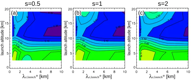
Fig. 5. Shown are for the Warner and McIntyre/CRISTA-1 comparison of horizontal GW-MF distributions correlation coefficients versus
altitude and model launch altitude for the choice of λ∗z,launch=2 km and s=0.5 (a), s=1 (b), and s=2.0 (c). Contour lines are: 0.2, 0.3, 0.4, 0.5, 0.6. launch altitude [km] altitude [km] launch altitude [km] altitude [km] launch altitude [km] altitude [km]
s=0.5
s=1
s=2
(a)
(b)
(c)
Fig. 6. Same as Fig. 5, but for CRISTA-2. Contour lines are: 0.2, 0.3, 0.4, 0.5, 0.6, 0.7, 0.75, 0.8.
an optimal set of parameters. This optimal set of parameters would have to fulfill two main criteria: high correlation of the horizontal distributions and comparable values of GW-MF.
It should also be noted that the CRISTA data sets are only about one week of data each and the results obtained in this paper are based on this limited data set only. This means some differences in the results could occur in other seasons and if meteorological conditions are different. However, there is evidence that the GW activity in August is similar in different years (Jiang et al., 2004b; Preusse et al., 2004; Preusse et al., 2006).
In addition, CRISTA GW-MF is available only in limited altitude regions of about 20–40 km for CRISTA-1 and 20– 50 km for CRISTA-2. This means the altitudes around the
mesopause where wind accelerations are maximum are not covered by the GW-MF data available.
4.1 Determination of an optimum model launch altitude by variation of s and λ∗z,launch
For the standard choice λ∗z,launch=2 km Figs. 5 and 6 show contour plots of the correlation coefficient between hori-zontal distributions of GW-MF of the Warner and McIntyre model and CRISTA as a reference. The results were ob-tained for the altitude range of available CRISTA GW-MF and seven different model launch altitudes from about 2.7 km to about 19 km (according to the UKMO pressure levels from 681 to 68.1 mbar).
launch altitude [km]
λ
z,launch* [km] launch altitude [km]λ
z,launch* [km] launch altitude [km]λ
z,launch* [km]s=0.5
s=1
s=2
(a)
(b)
(c)
Fig. 7. Warner and McIntyre/CRISTA-1 comparison of horizontal GW-MF. Correlation coefficients as shown in Fig. 5 are averaged over the
whole altitude range 22–37 km. Varied are model launch altitude and λ∗z,launchfor s=0.5 (a), s=1 (b), and s=2.0 (c).
I.e., the correlation coefficients of Figs. 5a–c averaged over the whole altitude range are the column at λ∗z,launch=2 km in Figs. 7a–c. Contour lines are: 0.2, 0.25, 0.3, 0.35, 0.4, 0.45. launch altitude [km]
λ
z,launch* [km] launch altitude [km]λ
z,launch* [km] launch altitude [km]λ
z,launch* [km]s=0.5
s=1
s=2
(a)
(b)
(c)
Fig. 8. Warner and McIntyre / CRISTA-2 comparison of horizontal GW-MF. Correlation coefficients as shown in Fig. 6 are averaged over
the whole altitude range 23–47 km. Varied are model launch altitude and λ∗z,launchfor s=0.5 (a), s=1 (b), and s=2.0 (c).
I.e., the correlation coefficients of Figs. 6a–c averaged over the whole altitude range are the column at λ∗z,launch=2 km in Figs. 8a–c. Contour lines are: 0.2, 0.25, 0.3, 0.35, 0.4, 0.45, 0.5, 0.55, 0.6, 0.65, 0.7.
Figure 5 shows the comparison with CRISTA-1 and Fig. 6 the comparison with CRISTA-2 GW-MF, respectively. Cor-relation coefficients are given for the spectral launch param-eters s=0.5 (a), s=1 (b), and s=2 (c). As can be seen from Figs. 5 and 6 for all choices of s: considering the whole range of measurement altitudes the correlation is highest for the second lowest launch level 464 mbar (launch latitude
∼5.4 km). It is also very high for the lowest launch level 681 mbar (launch latitude ∼2.7 km). Since this result is sim-ilar also for other choices of launch parameters λ∗z,launch and
s(not shown) we average the correlation coefficients over all altitudes for further comparisons.
Results based on this vertical averaging are shown in Figs. 7 and 8 for CRISTA-1 and CRISTA-2, respectively. Figures 7a–c and 8a–c show contour plots of the correlation coefficient averaged over the whole altitude range for differ-ent launch levels and differdiffer-ent values of λ∗z,launch. Figures 7 and 8 show the results for the choice (a) s=0.5, (b) s=1, and (c) s=2. Again, from these figures it can be seen clearly that the correlation is highest for the lowest two launch levels 681
(a)
λ
z,launch* = 2 km
(b)
λ
z,launch* = 4 km
(c)
λ
z,launch* = 6 km
zonal mean
λ
z*
[km]0 5 10 15 20
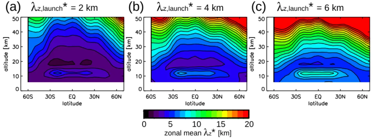
Fig. 9. Zonal mean cross section of λ∗z obtained from the Warner and McIntyre scheme (launch level 464 mbar, s=1) for the direction of maximum GW-MF during CRISTA-1 (no observational filter applied) and λ∗z,launch=2 km (a), λ∗z,launch=4 km (b), and λ∗z,launch=6 km (c).
(a)
λ
z,launch* = 2 km
(b)
λ
z,launch* = 4 km
(c)
λ
z,launch* = 6 km
zonal mean
λ
z*
[km]0 5 10 15 20
Fig. 10. Same as Fig. 9 but for Warner and McIntyre model GW-MF during CRISTA-2.
and 464 mbar (∼2.7 and ∼5.4 km) with the 464 mbar launch level giving the best results.
This means that the launch level 464 mbar (∼5.4 km) is the best choice for both CRISTA-1 and CRISTA-2 and is some kind of compromise for a globally fixed value of the launch altitude. This is valid for almost all choices of λ∗z,launchand s. Consequently, this launch level will be used for all following investigations.
4.2 Altitude dependence of λ∗z
To determine the correct value of λ∗z,launch=2π/m∗launch di-rect comparisons with measurements of the spectral shape of the GW vertical wavenumber spectrum would be highly desirable. Figure 9 shows latitude altitude cross sections of zonal mean λ∗z for the CRISTA-1 period (November 1994) obtained from the Warner and McIntyre scheme with the GW launch parameters s=1, launch level 464 mbar (∼5.4 km) and the choices λ∗z,launch=2 km (a), λ∗z,launch=4 km (b), and
λ∗z,launch=6 km (c). Figure 10 shows the same, but for the CRISTA-2 period (August 1997).
The Warner and McIntyre scheme calculates values mi*
for all directions i, in which GW-MF is derived. In this pa-per always 4 directions are used (corresponding to the cardi-nal points). The values of m* used to calculate the values of
λ∗z shown in Figs. 9 and 10 were obtained by calculating a mean of the single mi* components weighted by the squares
of the associated GW-MF components without CRISTA ob-servational filter applied. This means the distributions shown in Figs. 9 and 10 are about what an ideal instrument would be measuring if the Warner and McIntyre model output would be the “truth”. However, it should be noted that, depending on the specific shape of the spectrum, the maximum of the GW-MF vertical wavenumber spectrum used in the Warner and McIntyre scheme can be located at vertical wavelengths somewhat larger than the values of λ∗zshown.
From Figs. 9 and 10 can be seen that, starting from
λ∗z,launchat the launch level 464 mbar, the value λ∗
z basically
increases with altitude. This well-known effect is caused by growth of the GW amplitudes with altitude, leading to an ex-tension of the saturated part of the vertical wavenumber spec-trum towards lower m (longer vertical wavelengths) at higher altitudes (Fritts and VanZandt, 1993; Gardner, 1994). In ad-dition, there are also meridional variations mainly caused by Doppler shift of the vertical wavenumber spectrum due to the vertical profile of the horizontal wind.
If the directions of horizontal wind and GW-MF are anti-parallel the vertical wavenumber spectrum (this means also the location of m*) is Doppler shifted towards lower values of m (higher λz) and wave breaking is reduced. Therefore
GW-MF for the GWs propagating opposite to the wind direc-tion can be higher than GW-MF for GWs with zero Doppler shift. This explains why for CRISTA-2 GW-MF is enhanced inside the southern polar jet and also the values of high GW-MF in the northern subtropics caused by subtropical east-erlies. The opposite way around, the vertical wavenumber spectrum of GWs propagating parallel to the direction of the prevailing wind is shifted towards higher values of m. In this case wave breaking is stronger and GW-MF is strongly reduced. Therefore the prevailing propagation direction of GWs inside the polar jet is opposite to the wind direction.
It is a general feature of the λ∗z distributions shown in Figs. 9 and 10 that for low values of λ∗z,launchthe average val-ues of λ∗zare lower over the whole altitude range. In addition, the meridional structure of λ∗z is more pronounced for low values of λ∗z,launch(cf. Figs. 9a and 10a) than for higher val-ues of λ∗
z,launch (cf. Figs. 9c and 10c). This means an
instru-ment with the capability to measure the vertical wavenum-ber spectrum from about λ∗
z. 2 km up to λ∗z& 20 km would
be able to resolve the vertical λ∗z distribution and could give directly constraints to the launch value λ∗z,launchby a compar-ison with model data. However, up to date there is no ex-perimental data set spanning such a wide interval of vertical wavelengths.
Some constraints can be inferred from the observations al-ready mentioned in Sect. 1 (Allen and Vincent, 1995; Hert-zog et al., 2001; Tsuda and Hocke, 2002). The experimental values of m* in the range of about 0.2–0.5 cycles/km (corre-sponding to λ∗z in the range 2–5 km) are valid for the lower stratosphere and mainly from low and mid-latitudes. If these values are compared to Figs. 9 and 10 we can conclude that the model parameter λ∗
z,launchshould not exceed about 4 km.
Otherwise the model values of λ∗
z would be too high in the
lower stratosphere.
Further constraints of the parameter λ∗z,launchcan be made by comparing measured and modeled distributions of GW-MF. Therefore a comparison of GW-MF absolute values from CRISTA and the Warner and McIntyre scheme will be made in the following subsection to find possible ranges of λ∗z,launch, and maybe to find even an optimum value for
λ∗z,launch.
4.3 Influence of λ∗
z,launch and s on horizontal correlations
and GW-MF absolute values 4.3.1 Variation of λ∗
z,launchand s
From Sect. 3 we have seen that the standard choice of GW launch parameters (s=1, λ∗
z,launch=2 km) used in the Warner
and McIntyre scheme already provides good agreement with the horizontal structures found in CRISTA GW-MF abso-lute values. To find out whether this agreement can be further improved and whether the low-bias of model GW-MF compared to CRISTA values can be reduced the values
λ∗z,launch=2π/m∗launchand s have been varied.
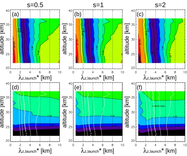
Figures 11a–c show deviations between horizontal dis-tributions of GW-MF absolute values calculated with the Warner and McIntyre scheme and CRISTA-1 GW-MF as a reference. The deviations shown are the slopes of linear fits through the origin from scatter plots of model GW-MF vs. CRISTA GW-MF for every pair of horizontal maps. The re-ciprocal of the slopes has been taken for slopes <1 (at low
λ∗z,launch) to have the same color scale for GW-MF deviations in both directions. The logarithm of the GW-MF values has been used for the fits to avoid over-weighting of low values of GW-MF (see also Ern et al., 2004, 2005).
The Warner and McIntyre GW-MF was calculated for the launch level 464 mbar and different altitudes and values
λ∗z,launch=2π/m∗launch.
Figure 11a is for s=0.5, (b) for s=1, and (c) for s=2. Low deviations (blue and purple colors) are found in the
λ∗z,launch range of about 2–5 km. Model values are lower than CRISTA-1 GW-MF to the left and higher to the right of the contour line labeled “1”. At values λ∗z,launch<1.5 km the model values are lower than the CRISTA-1 values by over a factor of 5–10 and outside the error margins. This deviation is too large to be compensated by other launch parameters. Therefore values of λ∗z,launch<1.5 km are not realistic. On the other hand for λ∗z,launch>6 km the GW-MF model values ex-ceed CRISTA-1 GW-MF by over a factor of 4–5, suggesting that also values λ∗z,launch>6 km are not realistic.
The different choices of s in Figs. 11a–c have almost no effect on this general behavior. Solely on average the model values for s=0.5 (Fig. 11a) are somewhat higher and the model values for s=2 (Fig. 11c) are somewhat lower than the results for s=1 (Fig. 11b). As a consequence, the con-tour line labeled “1” is slightly shifted towards lower values of λ∗z,launchfor s=0.5 and towards higher values λ∗z,launch for
s=2.
In Figs. 11d–f correlations between the horizontal distri-butions of Warner and McIntyre and CRISTA-1 GW-MF ab-solute values are shown for (d) s=0.5, (e) s=1, and (f) s=2. Similar as in Fig. 5 the correlation increases with altitude. Except for the lowest values λ∗
z,launch <1 km the correlation
is almost independent from λ∗z,launch.
In Figs. 12a–c the deviations of GW-MF values between model and instrument for the 464 mbar launch level are given
altitude [km]
λ
z,launch*
[km]
(d)
altitude [km]
λ
z,launch*
[km]
(e)
altitude [km]
λ
z,launch*
[km]
(f)
altitude [km]
λ
z,launch*
[km]
(c)
altitude [km]
λ
z,launch*
[km]
(b)
altitude [km]
λ
z,launch*
[km]
(a)
s=0.5
s=1
s=2
Fig. 11. Shown are for the Warner and McIntyre/CRISTA-1 comparison versus altitude and λ∗z,launch=2π/m∗launch:
(a–c) deviations of the Warner and McIntyre GW-MF absolute values (launch level 464 mbar) from CRISTA-1 as a reference, reciprocal
taken from values <1 (at low λ∗z,launch). Contour lines are 1, 1.5, 2, 3, 4, 5, 10, 100, and 1000.
(d–f) correlations between the horizontal distributions of Warner and McIntyre and CRISTA-1 GW-MF absolute values. Contour lines are:
0.2, 0.3, 0.4, 0.5, 0.6, 0.7, 0.75, 0.8. Overplotted white contour lines are the 1, 2 and 4 contour lines for the deviation of absolute values shown in (a–c).
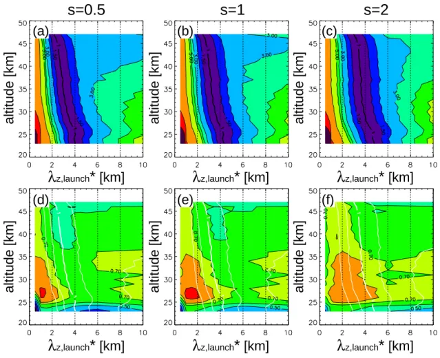
for the CRISTA-2 case. Again, (a) shows the results for
s=0.5, (b) for s=1, and (c) for s=2. The general behavior is similar as for the CRISTA-1 comparison. However, there is a tilt between CRISTA-2 and model GW-MF absolute val-ues with altitude (about a factor of 2 from 25 to 45 km). For the Warner and McIntyre/CRISTA-2 comparison even val-ues of λ∗z,launchas high as 8–10 km would be possible without too serious deviations between the magnitudes of model and CRISTA-2 GW-MF values. Again, the choice of s causes only minor shifts of the absolute values.
Figures 12d–f show the correlation coefficients for the model vs. CRISTA-2 comparison with model launch level 464 mbar. The behavior of the correlation coefficients is completely different from the results obtained for the CRISTA-1 comparison. For CRISTA-2 correlation is max-imum for low values of λ∗z,launch, minimum for λ∗z,launch in the range of about 4–8 km, and there is again higher
corre-lation (but less pronounced) for λ∗z,launch >8 km. The exact location of the maxima and minima changes with the choice of s. Especially the choice of s=2 produces a broader range of maximum correlation at values λ∗z,launchin the range from about 1–4 km.
4.3.2 Variation of λ∗z,launchand s: discussion of results Determining a best choice global set of launch parameters for the Warner and McIntyre scheme, i.e. suitable values of
λ∗z,launch, s and the launch level, means to weight the differ-ent results appropriately and to compromise between the two CRISTA flights. This will be aimed at in the following dis-cussion. To decide whether a certain combination of λ∗z,launch and s provides good agreement of CRISTA and model GW-MF two criteria have to be fulfilled.
altitude [km]
λ
z,launch*
[km]
(d)
altitude [km]
λ
z,launch*
[km]
(e)
altitude [km]
λ
z,launch*
[km]
(f)
altitude [km]
λ
z,launch*
[km]
(c)
altitude [km]
λ
z,launch*
[km]
(b)
altitude [km]
λ
z,launch*
[km]
(a)
s=0.5
s=1
s=2
Fig. 12. Shown are for the Warner and McIntyre / CRISTA-2 comparison versus altitude and λ∗z,launch=2π/m∗launch:
(a–c) deviations of the Warner and McIntyre GW-MF absolute values (launch level 464 mbar) from CRISTA-2 as a reference, reciprocal
taken from values <1 (at low λ∗z,launch). Contour lines are 1, 1.5, 2, 3, 4, 5, 10, 100, and 1000.
(d–f) correlations between the horizontal distributions of Warner and McIntyre and CRISTA-2 GW-MF absolute values. Contour lines are:
0.2, 0.3, 0.4, 0.5, 0.6, 0.7, 0.75, 0.8. Overplotted white contour lines are the 1, 2 and 4 contour lines for the deviation of absolute values shown in (a–c).
Warner and McIntyre values of GW-MF can be used (ab-solute value criterion). The deviation between CRISTA and Warner and McIntyre results should not exceed a factor of about 4–5 given by the error ranges of the data. The distri-bution of the correlations shown in Figs. 11 and 12 can serve as a second criterion (correlation criterion): The ranges of
λ∗z,launchwith the highest correlation will be favored. The general behavior of the GW-MF deviations, apart from some tilt with altitude between CRISTA and model GW-MF values and some shifts in the model value due to different choices of s, is as follows: The deviations are min-imum for λ∗z,launch in the range of about 2.5–4 km, model values are too low for about λ∗z,launch<2 km and too high for λ∗z,launch>6–10 km. More exact values for the different choices of s are summarized in Table 1 in the column for the absolute value criterion. This gives a first constraint to the possible range of λ∗z,launch.
As can be seen from Figs. 11a–c for the CRISTA-1 case there are almost no further constraints from the correlation criterion.
There is much stronger variation of the correlation for CRISTA-2. Usually there is a region of high correlation at low values of λ∗z,launch ranging from low to high alti-tudes and also a region of higher correlation at values of
λ∗z,launch>6 km. The region at high λ∗z,launchshows high cor-relation only at altitudes 25–40 km and corcor-relation is lower at lower and higher altitudes. Nevertheless, this region is listed in Table 1 for the sake of completeness.
Resulting λ∗z,launch ranges (see Table 1) have been deter-mined by combining the limitations given by the absolute value and the correlation criterion. In addition, the resulting ranges have been limited to values of λ∗z,launch≤4km because values of λ∗z,launchhigher than about 4 km result in too high
Table 1. Possible λ∗z,launchranges for the second lowest launch level (464 mbar, i.e. ∼5.4 km).
s λ∗z,launchrange [km] λz,∗launchrange [km] resulting λ∗z,launchrange [km] optimum (absolute value criterion) (correlation criterion) both criteria combined, cutoff 4 km λ∗z,launch[km] CRISTA-1 0.5 2.0–6.0 1.0–10.0 2.0–4.0 2.5–4.0 1 2.0–6.5 1.0–10.0 2.0–4.0 2.5–4.0 2 2.5–7.0 1.5–10.0 2.5–4.0 3.0–4.0 CRISTA-2 0.5 2.5–10.0 1.0–2.0 and 6.0–10.0 – – 1 2.5–10.0 1.0–3.0 and 7.0–10.0 2.5–3.0 2.5 2 2.5–10.0 0.5–10.0 2.5–4.0 2.5–3.0
From Table 1 we can see that for CRISTA-2 and s=0.5 the resulting range is empty. In the regions of high correlation the deviations from the CRISTA-2 GW-MF values are too large. This indicates that a common global value of s=0.5 would not be a good choice. Combining the resulting ranges of CRISTA-1 and CRISTA-2 for s=1 and s=2 gives us pos-sible λ∗z,launch ranges of about 2.5–3 and 2.5–4 km, respec-tively. However, for CRISTA-2 and s=1 as a compromise we have to accept somewhat reduced correlation at altitudes above 35 km. This situation is improved for s=2.
We have also determined optimum ranges of λ∗z,launch(see Table 1) by considering only the part of the resulting ranges with deviations less than a factor of about 2 for CRISTA-1. For CRISTA-2 it is more important to choose λ∗
z,launch in
a way to obtain correlation as high as possible from low to high altitudes.
Therefore we choose as optimum values for CRISTA-2 the lower limit of the resulting λ∗z,launch ranges. Com-bining the optimum values from 1 and CRISTA-2 gives us optimum values of λ∗z,launch=2.5 km for s=1 and
λ∗z,launch=3.0 km for s=2.
As can be summarized, a common global value of λ∗z,launch lower than about 2.0–2.5 km is unlikely because model GW-MF is too low compared to CRISTA GW-GW-MF. On the other hand, to preserve the high correlation for the CRISTA-2 case at low λ∗z,launch, an increase of λ∗z,launchto values over about 3 km does not seem to be justified. This gives us a quite nar-row range of λ∗z,launchwhich is compatible with both CRISTA missions for s=1 and s=2. Since s=2 gives the largest result-ing range of λ∗z,launch this value might be better suited than
s=1. For s=0.5 no resulting λ∗z,launch range can be found for CRISTA-2. This means values of s and λ∗z,launch somewhat higher than the standard values s=1 and λ∗
z,launch=2 km are
the best choice.
Optimum values of λ∗z,launch=2.5–3.0 km still produce a notable low-bias (about a factor of 2–3) of the model
GW-MF compared to CRISTA GW-GW-MF. This low-bias could be reduced, for example, by increasing the model parameter β (see Sect. 1) by a factor of 2. However, it should also be kept in mind that CRISTA GW-MF could be somewhat high-biased due to additional GW sources (e.g., mountain waves) not considered in the parameterization scheme and that devi-ations of a factor of 2–3 are inside the error limits.
5 Influence of λ∗z,launchand s on the vertical distribution of GW drag
One of the main purposes of a GW parameterization scheme is to provide realistic values of GW drag so that winds calcu-lated in GCMs are more reliable. In this section we investi-gate whether the ranges of λ∗z,launchand s derived in the previ-ous section are compatible with measurements and theoret-ical considerations. To check whether the different choices of launch parameters discussed above give reasonable re-sults the zonal mean zonal GW drag has been calculated for some selected cases. As atmospheric background the same composite wind and temperature field was used as in (Preusse et al., 2006): From 0–28 km altitude European Cen-tre for Medium-Range Weather Forecasts (ECMWF) reanal-yses were used (Coy and Swinbank, 1997). For altitudes 20– 85 km CRISTA-2 temperatures and geostrophic wind derived from CRISTA-2 data were used (Oberheide et al., 2002). Above 70 km COSPAR International Reference Atmosphere (CIRA) climatological data were used (Chandra et al., 1990). At the overlapping altitudes smooth transitions were gener-ated by applying weighted means.
The results obtained from the Warner and McIntyre scheme are shown in Fig. 13.
The peak values of GW drag are about the same in all cases shown, however, there are significant differences in the ver-tical distributions of GW drag.
-60 -40 -20 0 20 40 60
zonal mean zonal GW drag [m/s/day]
(a)
λ
z,launch*=2 km, s=0.5
(b)
λ
z,launch*=2 km, s=1
(c)
λ
z,launch*=2 km, s=2
(f)
(e)
(d)
λ
z,launch*=1 km, s=1
λ
z,launch*=4 km, s=1
λ
z,launch*=4 km, s=2
Fig. 13. Zonal mean zonal GW drag in m/s/day calculated with the Warner and McIntyre GW scheme for the CRISTA-2 case (August 1997)
with launch level 464 mbar. Shown are results for the launch parameter combinations: (a) λ∗z,launch=2 km and s=0.5, (b) λ∗z,launch=2 km and
s=1, (c) λ∗z,launch=2 km and s=2, (d) λ∗z,launch=1 km and s=1, (e) λ∗z,launch=4 km and s=1, (f) λ∗z,launch=4 km and s=2.
Figures 13a–c show the influence of different values s for fixed λ∗z,launch=2 km. For s=0.5 (Fig. 13a) GW-MF is higher in the unsaturated part of the launch spectrum than for the standard case with s=1 (Fig. 13b). Therefore for s=0.5 a larger part of the GW spectrum is saturated already at lower altitudes, leading to somewhat higher GW drag already at lower altitudes than in the standard case (see Figs. 13a and b). Accordingly, for s=2 (Fig. 13c) a shift of high GW drag towards higher altitudes would be expected because GW-MF in the unsaturated part of the launch spectrum is reduced and GW breaking postponed towards higher altitudes. Compar-ing Figs. 13b and c this is observed, indeed.
Figures 13d–f show the influence of different λ∗z,launchon the GW drag vertical distribution. The results of Fig. 13d were obtained with λ∗z,launch=1 km and s=1. This means a larger part of the launch spectrum is unsaturated. And, as expected, in Fig. 13d the regions of GW breaking and high GW-MF are shifted to higher altitudes than in the standard case with λ∗z,launch=2 km and s=1 (Fig. 13b). For example, in Fig. 13d at the southernmost latitudes there is a peak of GW drag at altitudes above 90 km and only moderate values of GW drag below. This distribution of GW drag does not seem to be realistic because there are indications for GW breaking already at lower altitudes of about 50–60 km at the top of the southern polar jet (Preusse et al., 2006). Therefore higher values of GW drag are expected already in the altitude region
50–60 km. This confirms that the choice of λ∗z,launch=1 km is too low.
In Fig. 13e the launch parameters were λ∗
z,launch=4 km and s=1. Choosing a higher value of λ∗
z,launchimplicates a larger
saturated part of the launch spectrum. Correspondingly in Fig. 13e already at altitudes as low as 30 km relatively high GW drag values of about 10–15 m/s/day can be found in the region of the southern polar jet. Increasing s to a value of 2 (Fig. 13f) cannot reduce this effect significantly.
Using a value of λ∗z,launch=10 km (not shown) leads to GW drag values of up to 50 m/s/day already at altitudes of 25 km. From theoretical considerations maximum values of about 2 m/s/day at these altitudes would be expected (e.g., Alexan-der and Rosenlof, 1996). Measurements can exceed this value by more than a factor of two (e.g., Sato, 1994). Nev-ertheless, the very high values of GW drag at low altitudes obtained for λ∗
z,launch=10 km seem to be unrealistic. An
in-crease of λ∗
z,launch over a value of about 4 km therefore does
not seem to make sense. This gives us another consistency check for the reasonable ranges of λ∗z,launchdeduced from Ta-ble 1.
In the Warner and McIntyre scheme the parameter β (see also Sect. 1) is proportional to the values of GW-MF as well as to the values of GW drag. Therefore scaling of GW-MF and GW drag with β as suggested in Sect. 4.3.2 can be used to reduce the low-bias of model GW-MF without
60N 40N 20N Eq. 20S 40S 60S
180W 120W 60W 0 60E 120E 180E 60N 40N 20N Eq. 20S 40S 60S
180W 120W 60W 0 60E 120E 180E
60N 40N 20N Eq. 20S 40S 60S
180W 120W 60W 0 60E 120E 180E 60N 40N 20N Eq. 20S 40S 60S
180W 120W 60W 0 60E 120E 180E
60N 40N 20N Eq. 20S 40S 60S
180W 120W 60W 0 60E 120E 180E 60N 40N 20N Eq. 20S 40S 60S
180W 120W 60W 0 60E 120E 180E
(a)
(b)
(d)
(f)
(c)
(e)
CRISTA-2
Warner & McIntyre
25 km 25 km 35 km 45 km 45 km 35 km 1.4 2.0 2.4 2.8 3.2 3.6 4.0 5.0 6.0 10 20 30 40 50 0.7 1.0 1.2 1.4 1.6 1.8 2.0 2.5 3.0 5.0 10 15 20 25 0.18 0.25 0.3 0.35 0.4 0.45 0.5 0.63 0.75 1.3 2.5 3.8 5 6.3 0.18 0.25 0.3 0.35 0.4 0.45 0.5 0.63 0.75 1.3 2.5 3.8 5 6.3 0.7 1.0 1.2 1.4 1.6 1.8 2.0 2.5 3.0 5.0 10 15 20 25 0.35 0.5 0.6 0.7 0.8 0.9 1.0 1.3 1.5 2.5 5.0 7.5 10 13
Fig. 14. Shown are horizontal distributions of GW-MF absolute values in mPa (see color bars and contour labels) for CRISTA-2 (August
1997) at altitudes of 25 km (a), 35 km (c), and 45 km(e). Also shown are horizontal distributions of GW-MF absolute values in mPa calculated with the Warner and McIntyre GW parameterization scheme at the same altitudes (25 km (b), 35 km (d), and 45 km (f)) for a fixed model GW launch level at 464 mbar (about 5.4 km) and the spectral parameters s=2 and λ∗z,launch=3 km. Instrumental visibility filtering has been applied to the model values. Please note that due to differences in the GW-MF absolute values contour lines and color codes are different at different altitudes and also different for CRISTA and model results.
Figure 3a was reproduced from Fig. 3d in: Ern, M., Preusse, P., Alexander, M. J., and Warner, C. D., Absolute values of gravity wave momentum flux derived from satellite data, J. Geophys. Res., 109, D20103, doi:10.1029/2004JD004752, 2004. Copyright [2004] American Geophysical Union. Reproduced by permission of American Geophysical Union.
0.35 0.5 0.6 0.7 0.8 0.9 1 1.3 1.5 2.5 5 7.5 10 13 60N 40N 20N Eq. 20S 40S 60S
180W 120W 60W 0 60E 120E 180E 60N 40N 20N Eq. 20S 40S 60S
180W 120W 60W 0 60E 120E 180E
60N 40N 20N Eq. 20S 40S 60S
180W 120W 60W 0 60E 120E 180E 60N 40N 20N Eq. 20S 40S 60S
180W 120W 60W 0 60E 120E 180E
(a)
(b)
(d)
(c)
CRISTA-1
Warner & McIntyre
25 km 25 km 35 km 35 km 1.4 2.0 2.4 2.8 3.2 3.6 4.0 5.0 6.0 10 20 30 40 50 0.35 0.5 0.6 0.7 0.8 0.9 1 1.3 1.5 2.5 5 7.5 10 13 1.4 2.0 2.4 2.8 3.2 3.6 4.0 5.0 6.0 10 20 30 40 50
Fig. 15. Horizontal distributions of GW-MF absolute values in mPa (see color bars and contour labels) for CRISTA-1 (November 1994) at
altitudes of 25 km (a) and 35 km (c). Also shown are horizontal distributions of GW-MF absolute values in mPa calculated with the Warner and McIntyre GW parameterization scheme at the same altitudes (25 km (b), 35 km (d)) for a fixed model GW launch level at 464 mbar about 5.4 km) and the spectral parameters s=2 and λ∗z,launch=3 km. Instrumental visibility filtering has been applied to the model values. Please note that due to differences in the GW-MF absolute values contour lines and color codes are different at different altitudes and also different for CRISTA and model results.
changing the relative distributions of GW-MF and GW drag. This means the correlation between modeled GW-MF and CRISTA GW-MF as reference is left unchanged and also the ranges of launch parameters determined from the correlation criterion.
Indeed, increasing of the model parameter β (see Sect. 1) to reduce the low-bias of model GW-MF as suggested in Sect. 4.3.2 makes sense because for the CRISTA-2 case peak values of acceleration calculated with the Warner and McIn-tyre scheme in the upper mesosphere are about 50 m/s/day for the standard launch parameters (see Fig. 13b) and only a little higher for the optimum launch parameters shown in Table 1. On the other hand monthly mean values of GW-MF derived from radar observations can be as high as 100– 200 m/s/day (Hocking, 2005). This means higher values of
β than the standard value of ∼0.1 are not in contradiction with observations. In fact, a value of β=0.2 would result in
peak values comparable to those reported by Hocking (2005). Another important point can be seen from Fig. 13: There are high values of GW drag not only in the winter hemi-sphere at the top of the southern polar jet, but also in the northern hemisphere where only little GW-MF was observed by CRISTA (see above) and also only low temperature vari-ances are observed at higher altitudes (Preusse et al., 2006). This means that GW-MF and GW drag are too high in the model results. Again, this is a clear indication that the as-sumption of a global launch distribution for GW parameter-ization schemes is too simple and global measurements of GW-MF especially in the mesosphere and the mesopause re-gion over a full annual cycle are in need to give further con-straints to the GW-MF launch distribution.
launch altitude [km] altitude [km] launch altitude [km] altitude [km] launch altitude [km] altitude [km]
s=0.5
s=1
s=2
(a)
(b)
(c)
Fig. 16. Shown are for the Warner and McIntyre/CRISTA-1 comparison of horizontal GW-MF distributions correlation coefficients versus
altitude and model launch altitude for the choice of λ∗z,launch=3 km and s=0.5 (a), s=1 (b), and s=2.0 (c). Contour lines are: 0.2, 0.3, 0.4, 0.5, 0.6. launch altitude [km] altitude [km] launch altitude [km] altitude [km] launch altitude [km] altitude [km]
s=0.5
s=1
s=2
(a)
(b)
(c)
Fig. 17. Same as Fig. 16, but for CRISTA-2. Contour lines are: 0.2, 0.3, 0.4, 0.5, 0.6, 0.7, 0.75, 0.8.
6 Summary and conclusions
In this paper absolute values of GW-MF derived from the CRISTA-1 (November 1994) and CRISTA-2 (August 1997) satellite missions have been compared to GW-MF absolute values calculated with the Warner and McIntyre GW pa-rameterization scheme for these two periods. Horizontal structures of GW-MF can be reproduced already by using the standard set of Warner and McIntyre launch parameters (λ∗z,launch=2 km and s=1) if a low launch level is used. For this standard set of launch parameters the model values of GW-MF are considerably lower, however, this set of param-eters is already some kind of compromise, considering the large error range of about a factor of 4–5 for the GW-MF absolute values.
The best correlation between CRISTA and Warner and
McIntyre horizontal distributions is achieved for the second lowest model launch level 464 mbar (i.e. about 5.4 km). This maximum correlation is a persistent feature for both CRISTA flights and almost all choices of spectral launch parameters
λ∗z,launchand s.
Possible ranges of λ∗
z,launchhave been determined by
opti-mizing the agreement of GW-MF absolute values as well as the correlation between CRISTA and model distributions of GW-MF and by considering the vertical distribution of λ∗z. The resulting range for λ∗z,launchis about 2–4 km, depending on s. The value s=2 gives better overlap between the ranges obtained for the absolute value criterion on the one hand and the correlation criterion on the other hand. Using the vertical distribution of GW drag as cross-check confirms the derived
(a)
(b)
λ
z,launch*
= 3 km, s=2.0
zonal meanλ
z*
[km]0
5
10
15
20
CRISTA-1
CRISTA-2
Fig. 18. Zonal mean cross section of λ∗zobtained from the Warner and McIntyre scheme (launch level 464 mbar, λ∗z,launch=3 km, and s=2) for the direction of maximum GW-MF during CRISTA-1 (a) and CRISTA-2 (b). No observational filter was applied.
λ
z,launch*
=3 km, s=2.0
-60 -40 -20 0 20 40 60
zonal mean zonal GW drag [m/s/day]
Fig. 19. Zonal mean zonal GW drag in m/s/day calculated with the
Warner and McIntyre GW scheme for the CRISTA-2 case (August 1997) using the optimum launch parameters: launch level 464 mbar,
λ∗z,launch=3 km and s=2.
This means there are some indications that λ∗z,launchshould be somewhat larger than the standard value of 2 km, but not very much larger (maybe λ∗z,launch=2.5–3.0 km). In addition, the parameter s should be increased to s=2, reducing the spectral power in the unsaturated part of the GW vertical wavenumber spectrum. The remaining low-bias of the model GW-MF with respect to the CRISTA estimates could be re-duced by increasing the model input parameter β by a factor
of about 2 (this would also increase the GW-MF values as well as the GW drag values by a factor of 2) without causing incompatibilities with radar observations of GW drag.
The choice of such a global set of model launch param-eters should be made with some caution for some reasons. First, the error ranges of GW-MF are relatively large, even though part of the error will be a systematic error and rela-tive variations of GW-MF in the horizontal distributions are highly significant. Of course, this large error range, as well as the fact that CRISTA is only a very limited data set of two weeks of measurements in a limited altitude interval, will put some uncertainty on the determined ranges of model param-eters. Second, the choice of a global set of launch parameters itself is a problem. Already from the CRISTA versus Warner and McIntyre model comparison there are some indications for localized GW sources which cannot be reproduced by the model. In addition, there are high values of model GW drag in northern latitudes and at the same time only little GW activity at high northern latitudes during CRISTA-2. This in-dicates that there should be some annual cycle in the GW sources at middle and high latitudes which is not incorpo-rated in the model.
Therefore we conclude that to overcome the limitation of GW parameterization schemes to a fixed set of launch param-eters detailed global measurements of the GW source distri-bution over a full annual cycle are highly desirable.