HAL Id: insu-01586126
https://hal-insu.archives-ouvertes.fr/insu-01586126
Submitted on 12 Sep 2017
HAL is a multi-disciplinary open access
archive for the deposit and dissemination of
sci-entific research documents, whether they are
pub-lished or not. The documents may come from
teaching and research institutions in France or
abroad, or from public or private research centers.
L’archive ouverte pluridisciplinaire HAL, est
destinée au dépôt et à la diffusion de documents
scientifiques de niveau recherche, publiés ou non,
émanant des établissements d’enseignement et de
recherche français ou étrangers, des laboratoires
publics ou privés.
Formation of the axial relief at the very slow spreading
Southwest Indian Ridge (49° to 69°E)
Mathilde Cannat, Celine Rommevaux-Jestin, Daniel Sauter, Christine Deplus,
Véronique Mendel
To cite this version:
Mathilde Cannat, Celine Rommevaux-Jestin, Daniel Sauter, Christine Deplus, Véronique Mendel.
Formation of the axial relief at the very slow spreading Southwest Indian Ridge (49° to 69°E). Journal
of Geophysical Research : Solid Earth, American Geophysical Union, 1999, 104 (B10),
pp.22,825-22,843. �10.1029/1999JB900195�. �insu-01586126�
JOURNAL OF GEOPHYSICAL RESEARCH, VOL. 104, NO. B10, PAGES 22,825-22,843, OCTOBER 10, 1999
Formation of the axial relief at the very slow spreading
Southwest Indian Ridge (49 ø to 69øE)
Mathilde
Cannat,
1 C•line
Rommevaux-Jestin,
1 Daniel
Sauter,
2 Christine
Deplus
3
and V•ronique Mendel2,
4
Abstract.
The comparison
of segment
lengths,
relief, and gravity
signature
along
the very slow
spreading
Southwest
Indian
Ridge (SWIR) between
49øE and 69øE suggests
that the marked
change
in segmentation
style
that occurs
across
the Melville transform
(60ø45'E)
reflects
a change
in the modes
of formation
of the axial topography.
We propose
that the axial relief east of Melville
is largely
due to volcanic
constructions
that load the axial lithosphere
from above.
By contrast,
the
axial relief in segments
west
of the Melville fracture
zone appears
to be primarily
due, as proposed
for segments
of the faster
spreading
Mid-Atlantic
Ridge,
to along-axis
changes
in the depth
of the
axial valley,
and to partial
compensation
of negative
loads
(thicker
lower crust
and/or
lighter
upper
mantle)
acting
within the plate, or at the bottom
of the plate. In terms
of geology,
this means
that
the contribution
of the uppermost,
effusive,
part of the crust
to along-axis
crustal
thickness
variations
may be greater
east
of Melville than in other
regions
of the study
area.
Regional
axial
depths
suggest
that the ridge
east
of Melville is also
characterized
by a low melt supply
and is
underlain
by cold mantle.
A simple
model of mantle
melting
and regional
isostatic
compensation
suggests
that differences
in mantle
temperature
and in melt thickness
between
this deep
eastern
ridge region,
and the shallower
region
west of the Gallieni transform
(52ø20'E),
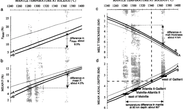
are of the order of
80øC and 4 km, respectively.
1. Introduction
The morphology of mid-ocean ridges is affected in systematic ways by changes in spreading rate: fast spreading ridges (full rates of 80 mm/yr or more) have an axial high, while slow spreading ridges (full rates of 40 mm/yr or less) generally have an axial valley [Macdonald, 1982]. Slow-spreading ridges also display more pronounced along-axis variations of axial depths and crustal structure than faster spreading ridges. Systematic studies of along-axis variations in axial topography [Fox eta/., 1991' Grindlay eta/., 1992; Semlg•r• eta/., 1993], gravity signature [Kuo and Forsyth, 1988; Linet
al., 1990; Rommevaux et al., 1994; Genre et al., 1995; Derrick
et al., 1995], and seismic velocity structure [Purdy and Derrick, 1986; Tolstoy eta/., 1993; Wolfe eta/., 1995] at the Mid-Atlantic Ridge (MAR) have led to the definition of a typical segment of this slow spreading ridge (full rate 24 to 40 mm/yr). The center of the segment is shallower, with a narrow to locally nonexistent axial valley, a mantle Bouguer anomaly (MBA) low, and Moho depths of 6 to 9 km. Segments ends are
l Centre
National
de la Recherche
Scientifique
UPRESA
7058,
Laboratoire de P6trologie., Universit6 Pierre et Marie Curie, Paris.
2Centre
National
de la Recherche
Scientifique
UMR
J0533,
Institut
de Physique du Globe, Strasbourg, France.
3Centre
National
de la Recherche
Scientifique
UMR 7577,
Laboratoire de Gravim•trie, Institut de Physique du Globe, Paris.
4Now
at Challenger
Division
for Seafloor
Processes,
Southampton
Oceanography Center, Southampton, England, United Kingdom. Copyright 1999 by the American Geophysical Union.
Paper number 1999JB900195.
0148-0227/99/1999JB900195509.00
marked by a wider and deeper axial valley, gravity highs, and a shallower Moho. Segments are 20 to 100 km long, and are generally limited by transform or nontransform offsets. Because crustal thickness variations are probably mainly due to along- axis variations of the magma supply, the segmentation of the MAR axis suggests that magma is not evenly distributed along-axis but focused toward the center of each segment [Kuo
and Forsyth, 1988; Linet al., 1990]. The focusing
mechanism
has been proposed
to be active mantle upwelling beneath
segments centers [Whitehead et al., 1984; Linet al., 1990] but remains a matter of debate [e.g., Magde et al., 1997].
Axial depths at a slow spreading ridge result from two
distinct mechanisms:
the partial isostatic
compensation
of
loads
emplaced
on top, within, and under
the axial lithosphere
(volcanic constructions, variations in the thickness of middle
and lower crustal
layers,
changes
in the density
of the upper
mantle beneath the ridge), and the extensional deformation of
this axial lithosphere
leading
to the formation
of a dynamically
supported axial valley. An intriguing characteristic of the
MAR is that, although
the general
presence
of a deep and wide
axial valley suggests
that the axial lithosphere
is strong
[Tapponnier
and Francheteau,
1978; Phipps Morgan et al.,
1987; Lin and Parmentier, 1989; Chen and Morgan, 1990],
the correlation
of along-axis
bathymetry
and gravity
variations
is good, suggests
near Airy compensation
of the along-axis
relief, and is therefore
consistent
with the axial lithosphere
being weak [Blackman and Forsyth, 1991; Neumann and Forsyth, 1993]. This apparent contradiction has been refered to by Neumann and Forsyth [1993] as the "paradox of the axial
profile".
The explanation
they proposed
for this paradox
is that
extensional
deformation
and the formation
of the axial valley
contribute
a significant
part of the MAR axial relief. The depth
of this axial valley being controlled
by the ridge's thermal
regime is correlated with magma supply and mantle
22,826 CANNAT ET AL.: AXIAL RELIEF OF SOUTHWEST INDIAN RIDGE 24øS 28øS 32øS 36øS 40øS 44øS
48øE 52øE 56øE 60øE 64øE 68øE 72'E
Figure 1. Shaded map of free air gravity anomalies derived from satellite altimetry [Sandwell and Smith, 1997]. Note the prominent off-axis traces of axial discontinuities between the
Gallieni and Melville fracture zones and the absence of a
similar pattern to the east and to the west.
temperature, hence with the gravity signature of the ridge axis. Numerical models of axial valley formation as a function of the ridge's thermal regime successfully reproduce the range of axial depth variations observed along the MAR and are therefore consistent with this hypothesis [Phipps Morgan et al., 1987; Lin and Parmentier, 1989; Chen and Morgan, 1990; Neumann and Forsyth, 1993; Shaw and Lin, 1996].
Our understanding of how slow spreading ridges work is to this date mostly based on studies of the MAR. The Southwest Indian Ridge (SWIR) has an even slower spreading rate (full rate 1.6 cm/yr [DeMets et al., 1990]) and has recently been mapped along a significant portion of its length [Munschy and Schlich, 1990; Mendel et al., 1997; Patriat et al., 1996; Grindlay et al., 1998]. In this paper, we analyze the axial relief and its gravity signature in the area comprised between 49øE (west of the Gallieni fracture zone) and 69øE (about 100 km to the west of the Rodriguez triple Junction; Figure 1). We use the bathymetry and gravity criteria developed in along-axis studies of the MAR to define axial segments, measure their along-axis relief and gravity signature, and use these data to propose that large volcanic edifices play a significant role in the formation of the SWIR axial relief. A passive upwelling, decompression mantle melting model is then used to estimate the range of large-scale along-axis variations in upper mantle temperature and magma production in the study area, assuming that axial depths, averaged over long portions of the ridge,
reflect isostatic balance. We use these estimates in a
discussion of what processes control the formation of the axial relief in different regions of the SWIR and of what this could imply for the geology of the crust in these regions.
2. General Setting of the Study Area
Bathymetry (Figure 2) and gravity data over the SWIR axis between 49 ø and 70øE have been acquired during three
cruises:
the Rodriguez
cruise
(RV Jean Charcot, 1984
[Munschy and Schlich, 1990]), the Capsing cruise L'Atalante, 1993 [Patriat et al., 1997]), and the Gallieni cruise (RV L-'Atalante, 1995 [Patriat et al., 1996]). Acquisition and processing of these data are described by Munschy and Schlich [1990], Mendel et al. [1997], and Rommevaux-Jestin et al. [1997]. The MBA was derived from merged shipboard free air anomaly (FAA) data from the three cruises, by subtracting the effect of the topography and of a Moho assumed to follow the topography with a constant 5 km crustal thickness [Rommevaux-Jestin et al., 1997].
Spreading rate (1.6 cm/yr) and spreading direction (NS) are constant in the study area [DeMets et al., 1990]. The SWIR has been propagating eastward at the Indian Ocean Triple Junction, and accretion ages therefore increase from east to west from about 5 Myr (A3) at 69øE, to about 64 Myr (A29) at 49øE [Patfiat and Segoufin, 1988; Sauter et al., 1997]. Other obvious variables in the spreading environment of different parts of the study area are the obliquity of the ridge axis (with respect to the normal to the spreading direction), and the presence or absence of long-lived transform and nontransform discontinuities. This last parameter is readily assessed from the satellite-derived FAA map (Figure l)[Sandwell and Smith, 1997]): - the ridge portion west of the Gallieni fracture zone (49øE to 52ø20'E) has an overall obliquity of 15 ø and is devoid of long-lived transform and nontransform discontinuities; - the ridge portion between the Gallieni and Melville fracture zones (52ø20'E to 60ø45'E) has an overall obliquity of 40 ø and comprises many long-lived transform and nontransform discontinuities; - and the ridge portion east of the Melville fracture zone (60ø45'E to 69øE) has an overall obliquity of 25 ø and is devoid of long-lived transform and
nontransform discontinuities.
3. Along-Axis Bathymetry and Gravity
Variations
Drawing a linear axis at a slow spreading ridge supposes that the plate boundary is, at least on a short timescale, linear, while the existence of an axial valley suggests instead that plate separation is accommodated within a zone of deformable lithosphere [Tapponnier and Francheteau, 1978; Phipps Morgan et al., 1987; Lin and Parmentier, 1989]. For the purpose of comparing along-axis bathymetry and gravity variations, however, we have drawn a linear axis, using conventions explained in Figure 3. This linear axis (Figure 2) represents the probable location of the most recent volcanic
activity
(neovolcanic
ridge
or center
of the axial magnetic
block) or the center of the axial deformation zone (deepest point of the axial valley). It differs only marginally from that used in previous along-axis studies of the area [Rommevaux- Jestin et al., 1997; Mendel et al., 1997] and is interrupted in three small regions (near 53øE, 62ø30'E, and 65øE; Figure 2) because of incomplete axial bathymetry coverage. A fourth gap at 66ø20'E corresponds to the overlap of two valleys, separated by a broad east-west trending ridge, 1500 m high [Mendel et al., 1997]. We have preferred to leave this 40-kin- long region out of our study because the nature of this broad ridge is uncertain: it exposes gabbroic rocks in its lower slopes [M•vel et al., 1997], it appears to be underlain by thin crust and therefore to be dynamically supported [Rommevaux- Jestin et al., 1997], but it has a clear normal polarity magnetic signature [Patriat et al., 1997] . We have also left the ridge portion between 69øE and the Rodriguez Triple Junction at
CANNAT ET AL.: AXIAL RELIEF OF SOUTHWEST INDIAN RIDGE 22,827 26 S 28'S 30'S 32'S 34øS 36'S 38'S 65OO 6000 55OO •,:.•. 5000
•..;•
4750
• .... 4500 • ;,.-: "" 4250 •;'"'• 4000!i•'
3500
•i•: 3000
':::" 2500 ::iii' 2000 80050'E 52'E 54øE 56'E 58'E 60'E 62'E 64'E 66'E 68'E 70'E
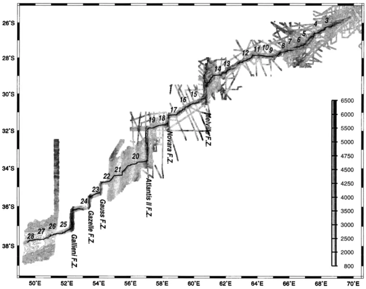
Figure 2. Southwest Indian Ridge bathymetry between 49øE and the Rodriguez Triple Junction (see text for references) with location of ridge segments 3 to 28. Black lines, ridge axis.
70øE out because its gravity signature is strongly influenced by the hotter thermal regime of the nearby Central and Southern Indian Ridges [Rommevaux-destin et al., 1997]. 3.1. Along-Axis Bathymetry Variations
Mean axial depths (obtained by averaging the axial depth profile in each region) decrease eastward from 3090 m west of the Gallieni fracture zone, to 4230 m between the Gallieni and
Atlantis II fracture zones, 4430 m between the Atlantis lI and
Melville fracture zones, and 4730 m east of the Melville fracture zone (Figure 4). This large-scale variation of axial depths suggests that the regional density structure of the axial region also varies, the ridge east of Melville being underlain by, on average, thinner crust, and/or denser mantle, than the ridge west of Gallieni. A broad positive anomaly of S waves
velocities, also consistent with a colder and thus denser
mantle, is observed in the eastern part of the study area [Debayle and L•v•que, 1997].
Short-wavelength variations of axial depths (Figure 4) have led us to define 26 segments (numbered 3 to 28, segments 1 and 2 being closer to the Rodriguez Triple Junction outside the study area; Figure 2). These segments are bounded by
transform faults or by nontransform and zero offset discontinuities. The boundary between two adjacent segments is defined as the deepest point in these discontinuities.
Nontransform discontinuities and zero offset discontinuities
AXIAL
•
Intrarift
ridge
•
- axial depth maximum depth - of axial domain depth below sea levelFigure 3. Schematic profile of the axial valley. The axis drawn
in Figure 2 is defined as the top of the intrarift ridge,
interpreted as a neovolcanic feature. In places where this intrarift ridge is absent, the axis is defined as the deepest point of the axial valley, and in the absence of an axial valley, as the center of the axial block of positive magnetization. Along-axis variations of axial depth and of the maximum depth of the axial domain are shown in Figure 4a.
22,828 CANNAT ET AL.: AXIAL RELIEF OF SOUTHWEST INDIAN RIDGE
o
N
CANNAT ET AL.: AXIAL RELIEF OF SOUTHWEST INDIAN RIDGE 22,829 34' 20'S 34' 40'S 27' 40'S 28' O0'S 31' O0'S 31' 20'S 55' O0'E 55' 20'E
63' 40'E 64' O0'E 64' 20'E 64' 40'E
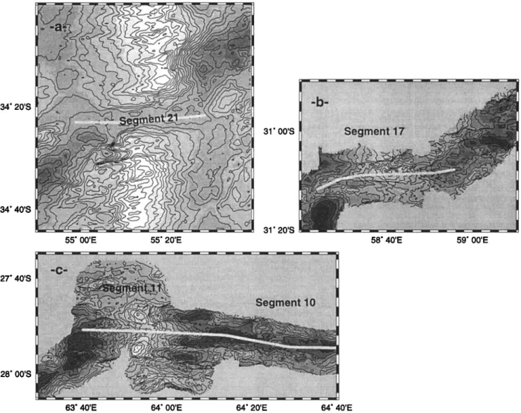
Figure 5. Bathymetry
of ridge segments
21, 17, and 10 and 11. Same
scale,
contour
interval
200 m. Dark grey,
depths
greater
than 5000 m; white, depths
shallower
than 2000 m. Solid grey lines show the location
of the
center
part of each
segment.
(a) Segment
21, (b) segment
17, and (c) segments
10 and 11. Segments
10 and 11
are separated
by a deep basin that does not correspond
to an offset of the ridge axis. See Figure 4 for
corresponding along-axis bathymetry and gravity profiles.
differ from those in the Atlantic [Mendel et al., 1997; Rommevaux-destin et al., 1997] in that they are generally longer in the along-axis direction. As an example, the nontransform discontinuity between segments 20 and 21 (Figure 4) is 110 km long, for an offset of 67 km. Nontransform discontinuities therefore make up significant portions of the along-axis length of many segments. In plan view (Figures 5a and 5b), a segment bounded by nontransform discontinuities is typically composed of a central, more elevated part that trends nearly east-west (perpendicular to the spreading direction), and of two deeper and more oblique (up to 45 ø in segments 16 and 21) distal parts. The overall trend of the segments varies between N55 ø (segment 21) and N96 ø (segment 10) and is generally of the order of N65 to N75 ø (Table 1).
It is worth noting at this point that there is no unique way to define ridge segments. Mendel et al. [ 1997], for example, have chosen to restrict their segments to the portions of the ridge axis that trend perpendicular to plate motion: that is, to
the central portions of the segments defined here. We have preferred to include the oblique portions of the axis (i.e., the wide nontransform discontinuities) in our definition, in order to work on a continuous axial profile similar to that taken into account in comparable along-axis studies of the Mid-Atlantic Ridge [Lin et al., 1990; Derrick et al., 199:5; Thibaud et al., 1998]. The definition chosen by Mendel et at. [1997] is, however, probably more consistent with the original definition of ridge segments as portions of the ridge limited by
axial discontinuities
[Macdonald
et al., 1988; Grindlay et al.,
1991' Semp•r• et al., 1993].
Figure 4 also shows along-axis variations of the maximum
depth of the axial domain,
which differs from axial depths
by
the height of the intra rift ridge (Figure 3). A coincidence or a near coincidence of the two depths in Figure 4 indicates either that there is no volcanic ridge, or only a very small one, in the
axial valley inner floor (this is commonly
the case
at segments
ends), or that there is no axial valley, or a very narrow and
22,830 CANNAT ET AL.' AXIAL RELIEF OF SOUTHWEST INDIAN RIDGE
Table 1. Length, Trend, Longitude at Western Extremity, Relief, and Along-Axis Variation of Mantle Bouguer Gravity Anomalies (AMBA) fk)r Bathymetric and Gravimetric Segments 3 to
28
Bathymetric Segments Gravimetric Segments
Segment Longitude Length, Trend, Relief, Longitude Length, Trend, AMBA,
E km N m E km N mGal 3 68.60 44.0 67.6 1833 (1437) 68.71 84.5 64.1 -35.8 4 67.87 38.9 67.6 1536 (1302) 67.95 101.7 53.8 -34.4 5 67.00 26.0 61.0 319 66.98 26.6 67.9 -6.5 6 66.78 42.6 74.6 1304 (898) 66.73 33.2 70.0 -12.2 7 66.12 26.2 86.8 851 66.12 28.3 78.4 -9.1 8 65.86 59.2 67.4 2581 (1914) 65.73 44.3/81 70.4 -24.2 9 64.95 26.4 93.1 574 64.95 26.4 93.1 -6.4 10 64.68 45.4 96.3 555 (327) 11 64.23 60.4 79.3 2672 64.68 104.7 86.6 -53.1 12 63.63 92.3 67.0 1185 14 61.77 65.1 66.0 2352 61.86 73.8 68.9 -40.4 15 60.32 73.6 67.0 1287 (920) 60.32 73.6 67.0 -31.1 16 59.62 71.6 57.1 1330 (975) 59.48 52.1 48.0 -16.4 17 58.99 63.2 64.4 2376 (1993) 58.95 54.6 76.2 -38.4 18 58.35 79.3 73.8 1840 (1676) 58.23 66.4 77.8 -35 19 57.55 47.5 70.9 1299 57.55 47.5 70.9 -14.6 20 57.02 145.3 66.2 1327 57.02 116.0 71.7 -42.1 21 55.59 88.9 54.8 1114 55.49 54.5 59.8 -32.9 22 54.80 61.5 69.8 934 54.80 61.5 69.8 -36.1 23 54.10 63.3 66.5 1150 54.10 63.3 66.5 - 13 25 52.25 91.4 69.9 1300 (1068) 52.25 91.4 69.9 -51.3 26 51.28 41.5 71.0 668 (475) 27 50.85 85.1 76.1 1895 50.85 85.1 76.1 -30.6 28 49.91 39.1 72.3 630 (504) 49.91 39.1 72.3 -10.7
Relief values between parentheses have been measured on an axial bathymetric profile that averages the axial depth and the maximum depth of the axial domain (as defined in Figure 3). Bathymetric segments 10,
12, and 26 do not have a gravity signature (see Figure 4).
and 27). Axial ridges are particularly prominent in the center of some segments, resulting in significant differences between the two depths (in segments 3, 4, 6, 8, 10, 15, 16, 17, 18, 20, 25, 26, and 28). The values listed between parentheses next to segment relief in Table 1 are reliefs calculated for an axial bathymetry profile that averages these two depths.
The length of most segments varies (Table 1) between 26 km (segment 5) and 92 km (segment 12). Segment 20 is exceptionally long (145 km). Its highest point (56ø30'E; Figure 2), however, is aligned with a north-south trending off- axis bathymetry low and gravity high that we interpreted as the trace of a small offset nontransform discontinuity. The volcanic ridge that goes down from there into the Atlantis II nodal basin appears to have recently propagated westward into the discontinuity. The present-day length of segment 20 therefore reflects a recent change in the local segmentation pattern, probably related to the persistent lengthening of the Atlantis II transform over the past 10 Myr [Dick et al., 1991 ].
Along-axis reliefs (Figure 6) vary between 319 m (segment 5) and 2672 m (segment 11). The topographic high in segment 23 has an even greater relief (2848 m) but is offset to the west
of the local MBA minimum and located near the intersection
with the Gazelle transform (Figure 4). We interpret this high as a tectonic feature (northern slope of the inside corner high associated to the Gazelle transform), not a volcanic ridge. The along-axis relief measured from the top of the less elevated volcanic ridge that does coincide with the MBA minimum for this segment (Figure 4) is of only 1150 m (Table 1).
As previously shown by Mendel et al. [1997], the segmentation pattern varies markedly across the Melville fracture zone (Figure 4). West of Melville, and particularly between the Gallieni and Melville fracture zones, along-axis
bathymetry variations look like those at the MAR, with relatively homogeneous segment lengths and along-axis relief (Figure 4). By contrast, segment length and relief east of the Melville fracture zone are highly variable: six segments
3500 + 4000 4500 + -10 (D -20 E :• -30 -40 Bathymetric segment •-• - Length ,• ... Length---• Gravimetric segment
Figure 6. Schematic along-axis bathymetry and mantle Bouguer gravity anomaly (MBA) profiles defining (top) the length and relief of a bathymetric segment, and (bottom) the length and AMBA of a gravimetric segment (values listed in Table 1).
CANNAT ET AL.: AXIAL RELIEF OF SOUTHWEST INDIAN RIDGE 22,831 (segments 5, 7, 9, 10, 12, and 13; 26 to 92 km in length) have
reliefs smaller than 1185 m; three segments (segments 3, 4, and 6; 39 to 44 km in length) have reliefs between 1304 and 1833 m (similar to the highest relief MAR segments); and three segments (segments 8, 11, and 14; 59 to 65 km in length) have reliefs between 2352 and 2674 m. These three very high relief segments are distant from one another by 190 km or more, the intervening segments (9, 10, and 12, 13; Figure 2) having much smaller reliefs (Figure 4).
3.2. Short Wavelength Along-Axis Gravity Variations
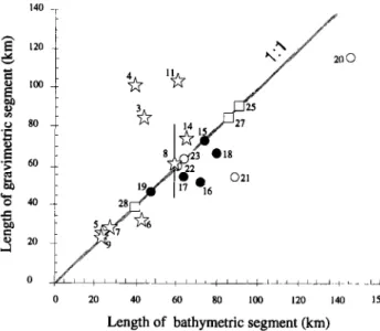
Short-wavelength variations in axial MBA also display the change in style associated with the Melville fracture zone, segments to the east of this fracture zone having a less regular pattern of MBA variations (Figure 4) [Rommevaux-destin et al., 1997]. In a typical MAR segment, the segment's ends correspond to topographic lows and to MBA highs and the segment's center corresponds to a topographic high and a MBA low [Lin et al., 1990]. In our study area, and particularly to the east of the Melville fracture zone, portions of the axis that are limited by two consecutive MBA maxima do not in every case coincide with the segment defined on the bathymetry (Figure 4). We will use the terms "gravimetric segments" or "gravimetric segmentation" for ridge portions limited by two consecutive MBA maxima (Figure 6). The length, trend, and amplitude (AMBA) of gravimetric segments in the study area are listed in Table 1. Segments 10, 12, and 26 are 41 to 92 km long, have reliefs of 554 to 1185 m, but do not correspond to a gravimetric segmentation. Gravimetric segment 3, 4, 11, and 14 are longer than corresponding bathymetric segments, while gravimetric segment 6, 16, 17, 18, 20, and 21 are shorter (Figure 7).
Segments 16, 20, and 21 are bounded at one or both ends by nontransform discontinuities characterized by wide MBA
140 _• E 120 .'x
•
•
4
1
•
"::•::"
'
ß • 6o ... == • ..• .... • 0 21•
l ,•" l l7 16
• 40 _ 28 0 • • • , • • {_t • , ,_•_••_z__•__•.•_••__ 4 .... 0 20 40 • 80 1• 120 140 150Length of bathymetric segment (km)
Figure
7. Length
of gravimetric
segments
(as defined
in Figure
6) versus the length of the corresponding
bathymetric
segments. Solid black line links the minimum and maximum
values
for the length
of gravimetric
segment
8 (see
text). Stars,
segments
located
to the east
of the Melville transform;
circles,
segments located between the Gallieni and Melville transfo•s
(solid circles,
east of Atlantis
II; open
circles,
west of Atlantis
II); squares, segments located to the west of the Gallieni transfo•.
highs with small saddle-shaped lows in the center (Figure 4). This configuration results in these segments being longer than corresponding gravimetric segments. Similarly, the MBA high at the eastern end of segment 18 is located a few kilometers to the west of the Novara ridge-transform intersection, while the MBA high at the western end of segment 14 is located a few kilometers to the east of the Melville ridge-transform intersection (Figure 4). We propose that this pattern is due, as proposed by Prince and Forsyth [1988] for local gravity lows observed in fracture zones of the Atlantic, to intense deformation and hydrothermal alteration reducing the density of crustal and upper mantle rocks in the transform region.
The length of gravimetric segment 8 is poorly constrained by available data because its western end coincides with a gap in the axial coverage (Figures 2 and 4). Axial MBA values may continue to increase westward to the higher values measured at the eastern end of segment 9 (Figure 4). This would make gravimetric segment 8 about 81 km long, with a AMBA of-24 mGal. Alternatively, axial MBA may reach a local maximum near the western termination of the bathymetric segment. This would make gravimetric segment 8 about 44 km long, for the same value of AMBA (Table 1).
The along-axis MBA low does not coincide with the topographic high in segments 3, 7, 8, 15, 18, 20, and 23 (Figure 4). In segment 23 the topographic high is probably an
inside comer tectonic structure related to the Gazelle transform
(Figure 4), and for the purpose of this study we have preferred to measure the relief of this segment from the top of the less prominent volcanic ridge that does coincide with the local MBA minimum (Table 1). We have done the same in segment 20, where the topographic high lies in the continuation of the off-axis trace of a discontinuity (Figure 2) and is inferred to be at least partly of tectonic origin. In segments 3, 7, 8, 15, and 18, however, seafloor morphology indicates that the central
topographic
highs are volcanic constructions
[Mendel et al.,
1997; Mendel and Sauter, 1997].
3.3. Segment Length, Segment Relief, and MBA Variations In this section, we discuss the formation of the axial topography, using the length and along-axis relief of
bathymetric
segments,
and the length
and AMBA of gravimetric
segments as defined in Figure 6 and listed in Table 1. Errors
made in measuring
these
values
on bathymetry
and MBA grids
are small with regards to variations induced by the choices made in the definition of the axis, and in the location of segment centers and ends. We therefore chose not to produce error bars for these measurements. However, we take into
account the smaller reliefs calculated for segments
with
prominent axial ridges by averaging axial depths and maximum
axial depths
(relief values
between
parentheses
in Table 1). We
allow for the length of gravimetric
segment
8 to vary between
44 and 81 km as it is not better constrained by available gravity data. We also allow for the length of gravimetric segments 16, 17, 18, and 21 to vary between their actual
length, and the (greater)
length of corresponding
bathymetric
segments. The idea being that the gravity signal due to partial compensation of the topography in these segments is overprinted by the effect of intense deformation and hydrothermal alteration in transform and nontransform domains near the segments ends. By using the length of the corresponding bathymetric segment, we approach the length the gravimetric segment would have had without this
22,832 CANNAT ET AL.' AXIAL RELIEF OF SOUTHWEST INDIAN RIDGE 3000 E •" 2500 E
(• 2000
'-
>, 1500 .c o 1000 ._e II n- 500 0 11 8 4 3 •oX -x 4 : .,:i•ii•ii•?•ß
.t.
!:i:
;;:•:i71.:•!
i:::.':71'
ii)!
:::i;4'
i•';•g•':'.":.:z!;:.::r ;: ::: ?:•i
'' •:':1':'""':":'::"::•':
' t '
' I'''
I ' ' ' I ' ' ' I
20 40 60 80 100 120
Length
of bathymetric
segment
(km)
Length
of gravimetric
segment
(km)
0 20 40 60 80 100 120 - 10 v •':. "•.• 23 ' ""::•':.:l• :..•.: :' ::':•f•i•s. :. ß 21_ •'. 22• • ... •'•i :•'•:•:•5•f: Q4 • ,
-50
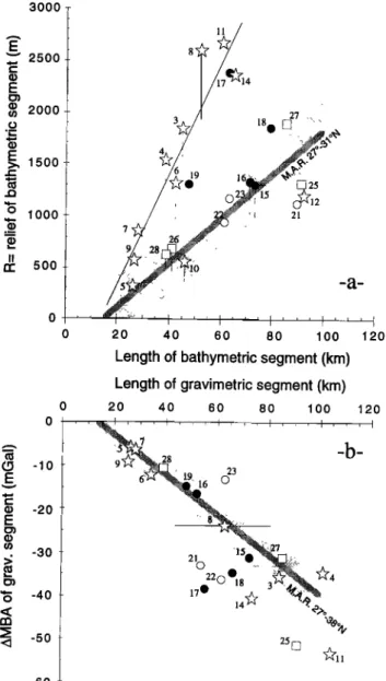
-60Figure 8. (a) Relief (R) versus
length
(L) of bathymetric
segments.
(b) Along-axis
variations
of mantle
Bouguer
gravity
anomalies
(AMBA) versus
length
of gravimetric
segment.
Symbols
as in Figure
7. Thick
grey
lines
are best
fitting
lines
proposed
for Mid-Atlantic
Ridge
segments
by Lin et aL [1990]
for Figure
8a (R- 0.0215L
- 323' pale
grey
areas,
+/_ 300 m),
and by Derrick
et al. [1995] for Figure
8b (AMBA- 0.45L + 5'
pale grey
areas,
+/. 5 regal).
The best
fitting
line (thin
black
line) for segments
3, 4, 5, 6, 7, 8, 9, 11, and
14 in Figure
8a is R
: 0.054L - 765 (correlation
coefficient:
0.916). Thin dotted
lines in Figure 8a show range of values between
the relief
measured as shown in Figure 6, and the relief measured on an
axial bathymetry
profile
that averages
the axial depth
and the
maximum
depth
of the axiaJ
domain
(as defined
in Figure
3).
Thin dotted lines in Figure 8b show minimum and maximumvalues
of the length
of gravimetric
segment
8 (see text), and
range
of values
between
the length
of gravimetric
segments
16,
17, 18, and 21 (as defined
in Figure 6). and the length
of
corresponding
bathymetric
segments
(see text).
deformation and alteration effect. Finally, we do not include segment 20 in this analysis, because its present-day length appears to result from the recent, and possibly ephemeral, propagation of a volcanic ridge into a nontransform discontinuity.
Compared to segments of the MAR [Lin et al., 1990; Neumann and Forsyth, 1993; Derrick et al., 1995; Thibaud et al., 1998], segments of the studied portion of the SWIR have similar lengths (20 to 100 km except for segment 20), a similar range of along-axis MBA variations (AMBA down to -53 mGal), but a wider range of along-axis reliefs (up to 2672 m; Table 1). Segments 3, 4, 11, and 14 have high reliefs and large AMBA (Figure 8), and their gravity signature has a longer length than the topography (Figure 7). Segment 8 is another high-relief segment of the east of Melville region, but it has a smaller AMBA, and the length of its gravity signal is not well constrained. Segment 17 is the only segment west of Melville with a relief greater than 2000 m (Figure 8a).
The relief (R) and the length (L) of MAR segments are roughly correlated [Blackman and Forsyth, 1991; Linet al.,
1990; Neumann and Forsyth, 1993; Thibaud et al., 1998], mean along-axis slopes (R/(L/2)) varying between 20 and 40 m/km. It is clear that most SWIR segments from the region east of Melville have higher relief to length ratios [Mendel et al., 1997] (Figure 8a), corresponding to mean along-axis slopes of up to 90 m/km. The exceptions are segments 10 and 12, which do not have a gravity signature, and segments 5 and 9 which are only 26 km long. By contrast, most segments west of Melville have mean along-axis slopes comparable to those of MAR segments (Figure 8a). The exception there is segment 17, and to a lesser extent segments 18, 19, and 27, which have steeper mean along-axis slopes. Segments 21 and 25 have mean along-axis slopes of less than 30 m/kin.
Segments
of the MAR also
show
a correlation
[Kuo and
Forsyth,
1988;
Lin et al., 1990;
Blackman
and
Forsyth,
1991;
Lin and
Phipps
Morgan,
1992;
Neumann
and Forsyth,
1993;
Detrick
et al., 1995; Wang
and Cochran,
1995;
Thibaud
et
al., 1998]
between
segment
length
and
AMBA
(Figure
8b).
This correlation
corresponds
to along-axis
mean MBA
gradients (AMBA/(L/2)) of 0.6 to 0.8 mGal/km. Most
gravimetric
segments
from the SWIR have similar
mean
MBA
gradients
(Figure
8b). Segments
11, 14, 17, 18, 21, 22, and
25,
however,
have
stronger
along-axis
mean
MBA
gradients
(up
to
1.4 mGal/km),
and
segment
23 has
a mean
MBA gradient
of
only 0.5 reGal/kin.
Stronger
mean along-axis
MBA gradients
indicate
that the
density
structure
varies
along-axis
more
rapidly
than
in other
segments.
This suggests
a more rapid along-axis
increase
of
crustal
thickness
and/or of mantle temperature
and melt
content.
Many segments
with strong
mean
MBA gradients
also
have
steep
mean
along-axis
slopes
(segments
11, 14, 17, and
18;
Figure
8). Conversely,
segments
3 and
4 have
mean
along-
axis
slopes
greater
than
78 m/km,
but mean
MBA gradients
of
only 0.6 to 0.8 mGal/km,
and segments
21, 22, and 23 have
strong
mean
MBA gradients
but moderate
to small
mean
along-
axis
slopes
(Figure
8a). The length
of the MBA signature
of
segment
8 (one
of the highest
relief
segment
in the study
area;
Figure
8a), and therefore
its along-axis
MBA gradient,
are
unfortunately not well constrained.
3.4. Along-Axis Crustal Thickness Variations
Mantle Bouguer anomalies
include components
due to
variations in crustal thickness, to variations in crustal
density,
and to variations
in mantle
density.
We do not have
enough
off-axis
gravity
and bathymetry
data
to produce
a grid
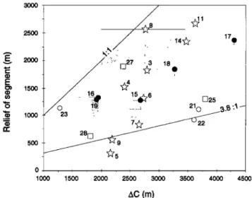
of residual MBA from which we could then derive crustal thickness variations in the study area. We therefore resorted to a crude analytical method and calculated variations in crustalCANNAT ET AL.' AXIAL RELIEF OF SOUTHWEST INDIAN RIDGE 22,833 3000 • 15oo 0 i , • , i , i , 1000 1500 2000 2500 3000 3500 4000 4500 ac (m)
Figure 9. Segment relief (R) versus the amplitude of crustal thickness variations (bC), calculated for each segment assuming that along-axis variations of mantle Bougucr gravity anomalies (AMBA) result from sinusoidal topography at the crest-mantle interface (see Appendix A). Symbols as in Figures 7 and 8. Thin dotted lines and pale grey areas correspond to the same range of variation in axial relief and in the length of gravimctric segments as in the diagrams of Figure 8.
thickness
(AC) within
each
segment,
assuming
that the gravity
signal is caused by sinusoidal variations in the thickness of aconstant
density
crust
(Pc
= 2700
kg/m
3) overlying
a constant
density
mantle
(Pro
= 3300 kg/m3).
In this calculation,
AC is
related to AMBA through a factor (see Appendix A) that
depends
on the wavelength
of MBA variations
(i.e., the length
of each gravimetric segment). The position of the various segments in Figure 9 is therefore a direct reflection of their position in the two diagrams of Figure 8.
The validity of this approach
is dependent
on how closely
MBA variations
approach
a sinusoidal
curve. It is apparent
in
Figure
4 that, in many segments,
MBA variations
are V-shaped
instead of being sinusoidal: this will bias AC estimates toward
higher values. Another, and potentially a more important,
problem is the continuation of the periodic pattern in the third dimension (perpendicular to the axis). Off-axis MBA data are scarce, but the lack of a regular off axis peak and trough pattern in the satellite FAA map to the east of Melville and to the west of Gallieni (Figure 1) suggests that crustal thickness at a given location along the ridge in these regions can vary over a relatively short timescale (this will bias AC estimates toward lower values). Finally, this approach does not take into account along-axis variations in mantle density due to the colder thermal regime near axial discontinuities and to possibly higher melt contents near segments centers: this will bias AC estimates toward higher values.
AC values shown
in Figure 9 must be appreciated
in the
light of these
limitations.
More reliable
AC values
will only be
obtained
through
three-dimensional
(3-D) models
(requiring
additionnal
off-axis gravity and bathymetry
data), instead
of
the 2-D model used here. AC varies between 3.5 km and more in segments 11, 14, 17, 21, 22, and 25, and 2 km and less in
segments
16, 19, 23, and 28. AC values
calculated
for segments
7 and 8 are within these two bounds and can be checked against actual seismic crustal thicknesses [Muller et al.,
1998]. The seismic
crustal
thickness
decreases
by about 2.5
km, and the average seismic velocity of the crust diminishes between the center and the ends of these segments [Muller et al., 1998]. Values of AC calculated from gravity data for segments 7 and 8 are of the same order. The decrease in crustal velocities observed toward segment ends has been documented previously along the MAR [Tolstoy et al., 1993; Detrick et al., 1995]. It probably goes together with a decrease
of crustal densities and should therefore cause AC calculated
from gravity data to be underestimated [Tolstoy et al., 1993; Detrick et al., 1995]. However, our crude method of calculating AC does not take into account the effect of having a colder, denser mantle at the ends of the segment, and this could balance the effect of these along-axis variations in crustal density.
3.5. Along-Axis Variations of the Depth of the Axial Valley and the Mode of Compensation of the Axial Relief
The axial relief (R) of a slow spreading ridge segment can be seen as the addition of two components: the isostatic response of the axial lithosphere to loads emplaced above, within, or below the plate (Ri); and rifting of the axial lithosphere producing a dynamically supported axial valley that deepens toward the segment's ends (Rv). If we could remove this dynamically supported component of the axial relief and consider only the response to isostatic loads (Ri) versus AC, the 1:1 line in the resulting diagram (Figure 10) would correspond to an uncompensated relief sitting on a plate without deflecting it, the 3.8:1 line would correspond to Airy
isostatic
compensation
(AC = ((Pro
- Pw)/(Pm
- Pc))R)
, and the
Ri:O baseline would correspond to an uncompensated negative load located under the plate.
Domains between the 1:1 and 3.8:1 lines, and below the
3.8:1 line in Figure 10, could then correspond to partial isostatic compensation of positive loads emplaced above the
_....•.:.•p
load
2500 ,• J
2000 , ) .• •7) • 25 • I 23 ' •'• • • 21,ooo
ac (m)Figure 10. Range of values discussed in text for the isostatic response component (Ri) of the axial relief (R), versus the amplitude of crustal thickness variations (AC), calculated for each segment assuming that along-axis variations of mantle Bouguer gravity anomalies (AMBA) result from sinusoidal topography at the crust-mantle interface (see Appendix A). Ri is inferred to be what is left of total relief (R) after removal of the component due to the dynamically supported axial valley (Rv). The Ri:O baseline corresponds to crustal thickening loading a rigid plate from underneath. The 1:1 line corresponds to relief sitting on a rigid plate. The 3.8:1 line corresponds to Airy isostatic compensation.
22,834
CANNAT
ET AL.:
AXIAL
RELIEF
OF SOUTHWEST
INDIAN
RIDGE
plate (plate
rigidity
prevents
the topography
in the center
of
the segment
to be as deep as it would
be in a local isostatic
compensation
mode)
and
of negative
loads
emplaced
below
the
plate (plate
rigidity
prevents
the topography
in the center
of
the segment
to be as high as it would
be in a local isostatic
compensation
mode), respectively.
We unfortunately
do not
have sufficient constraints on the values of Rv in our studyarea to actually plot each segment
on this Ri versus
AC
diagram. This would require sufficient knowledge
of
lithospheric
rheology
and thermal
structure
to model
axial
valley depths
and their along-axis
variations
[Neumann
and
Forsyth, 1993; Shaw and Lin, 1996]. Specifically, we have noconstraints on the thermal and mechanical effect of the broad
and large offset nontransform discontinuities that are typical of the very slow spreading SWIR, nor do we have natural seismicity constraints on axial lithospheric thickness along this ridge.
The range of Ri values shown in Figure 10 extends from Rv equal zero (Ri = R), an improbable end-member given the occurrence of well-developed nodal basins at the end of most SWIR segments [Mendel et al., 1997] (Figure 5), to Rv equal R minus the mean along-axis relief of a MAR segment of similar length (thick grey line in Figure 8a). This range of Ri values is based on two assumptions: (1) that Rv values for segments of the SWIR should be similar to Rv values of MAR segments of similar lengths; and (2) that the Rv value of a MAR segment is at the most equal to the whole measured relief (R) of this segment. This second assumption is consistent with the conclusions of thermomechanical modeling of MAR axial valley depths by Neumann and Forsyth [1993]. The first assumption is based on the observation that along-axis MBA gradients in most SWIR segments are similar to those of MAR segments (thick grey line in Figure 8b). This suggests that, for a given segment length, the contrast in lithospheric and
crustal thickness between the center and the extremities of a
segment is similar at the SWIR and at the MAR. Because variations of the depth of the axial valley are thought to be caused by along-axis variations of axial lithospheric thickness and crustal rheology [Phipps Morgan et al., 1987; Lin and Parrnentier, 1989; Chen and Morgan, 1990; Neumann and Forsyth, 1993; Shaw and Lin, 1996], similar MBA gradients suggest that the axial valley component (Rv) of the axial relief is of the same order of magnitude at the SWIR and at the MAR.
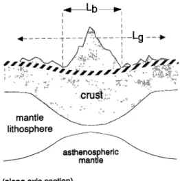
The range of Ri values shown in Figure 10 for high relief segments east of Melville (segments 3, 4, 8, 11, and 14) and for segments 17 and 19 between Melville and Atlantis falls entirely or almost entirely between the 1:1 and 3.8:1 lines, suggesting a predominant role of top loads in the isostatic response of the axial region. By contrast, the range of Ri values for lower relief segments (segments 5 and 9 east of Melville and segments 21, 22, 25, and 28 west of Atlantis) falls almost entirely beneath the 3.8:1 line, suggesting a predominant role of bottom loads. Flexural response to loads emplaced above the plate could also explain the difference in length of gravimetric and bathymetric segments 3, 4, 11, and 14 (Figures 7 and 11). In terms of geology, a dominance of top loads suggests a higher relative contribution of volcanic constructions loading the plate from above, with respect to crustal material or lighter mantle emplaced at deeper levels within or beneath the plate, to along-axis crustal thickness variations. In high relief segments east of Melville, and in segments 17 and 19 between Melville and Atlantis, the contribution of the uppermost,
•_
mantle
mantle
..•
lithosphere asthenosp mantle(along axis section)
Figure 11. Schematic along-axis section of a high relief SWIR segment east of the Melville transform. A large axial volcanic construction loads the plate and deflects it. Thick hatched line, top of deflected plate. Additional loading at Moho level (thickening of crust at segment center) and in upper mantle (thinner mantle lithosphere and possibly lighter asthenospheric mantle beneath segment center) also contribute to along-axis variations of mantle Bouguer gravity anomalies. Length of the bathymetric segment (Lb) is shorter than length of the corresponding gravimetric segment (Lg) due to flexural response of the plate and to along-axis extent of Moho and sub-Moho loads. Thinning of mantle lithosphere at segment center is due to excess magmatism causing the axial thermal regime to be hotter there. Asthenospheric mantle may be lighter beneath segment center due to higher temperatures and larger melt content.
effusive, part of the crust to along-axis MBA variations would therefore be greater than in the other segments of the studied area (Figure 11).
The existence of volcanic constructions that load the axial
lithosphere from above in segments 3, 4, 8, 11, 14, 17, and 19 is also consistent with observations made on bathymetric maps (Figures 5b and 5c). The axial valley floor in these segments does not have an hourglass shape [e.g., Semp•r• et al., 1993]. Instead, it has a width (measured in a north-south direction, parallel to spreading) of 10 to 20 km over most of the segment length [Mendel et al., 1997], and it does not narrow (as in the hourglass shape) near the center of the segment but appears to be filled by rounded or elongated reliefs that bear numerous volcanic cones [Mendel and Sauter, 1997]. This setting suggests that topographic highs in the center of these segments do not represent the floor of a narrow and shallow axial valley but are volcanic edifices filling a rather wide and deep axial valley.
4. Regional Variations in Axial Depth, Melt
Thickness and Mantle Temperature
Long-wavelength variations in axial depths reflect regional changes in the axial density structure, which is controlled by crustal thickness and by the density of the underlying mantle. The large-scale eastward deepening of the axis in the study area (Figure 4) therefore suggests that average crustal thicknesses and/or mantle temperatures beneath the ridge decrease from west to east. In this section we relate magma
CANNAT ET AL.: AXIAL RELIEF OF SOUTHWEST INDIAN RIDGE 22,83:5
Temperature (øC) melting rate (%)
1100 1150 1200 1250 1300 1350 1400 1450 0 5 10 15 20 25 30
20
,
20
.. 30 30 cold mantle: ß • 0.8 cm/yr6o
6o
+
...
...
hot mantle:80
Tsol:
1400oc
• 80}
I I I I I I I I I
90 90Figure 12. Temperatures and melting rates calculated.as a function of depth with the 1-D conductive cooling and melting model outlined in Appendix B, for two end-member mantle temperatures at solidus' cold mantle
(Tso
I - 1240øC)
and hot mantle
(Tso
I - 1400øC).
Cases
A and B correspond
to two conductive
cooling
settings
(see text and Appendix B). Temperatures and melting curves for adiabatic (ad.) melting are shown for •,uit•patiauit. •-t._ _, .... '- -' ... '-- eometr of" .... I 111Z IMk•;tkll •uw• tll•; g y mc : cuu,,t,• ' ... -' .... ' ... -'-' -with a a,,u n,c,t,n• ,,,uuc,, we dge angl e
of 45
ø and
a mantle
upwelling
velocity
equal
to the
hall'
spreading
rate.
Zf is the
depth
at the
top
of the
melting
domain.
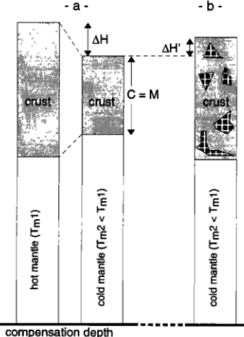
-a- -b-
compensation depth
/tH
Figure 13. Sketch of isostatically balanced columns for the calculation of regional axial depths. (a) The crust is made only of magmatic rocks. AH (difference in regional axial depth) therefore results only from differences in melt thickness (M- crustal thickness) and in mantle temperature (see Appendix B). (b) The crust also includes a proportion (S) of serpentinized mantle-derived peridotites (black squares). AH' relative to a setting with similar •nantle temperature and melt thickness but
no serpentinites
in the crust
is expressed
as (Pro-Pc)
/ (P,, -Pw)
MS/(1-S).
budget,
mantle temperature,
and regional
axial depth, in order
to better constrain what regional changes in mantle
temperature
and magma supply may accompany
the changes
observed in the axial segmentation pattern across the Melville
fracture
zone. We make the following
hypotheses:
- that the
rate of decompression
melting
in the mantle
at any given depth
above the solidus is proportional to the difference between the
solidus
temperature,
and the temperature
that would prevail at
that depth had no melting occurred
(Figure 12); - that the
regional pattern of mantle upwelling beneath the SWIR corresponds to passive flow (this assumption does not
preclude
active mantle flow at the scale of segments);
- that
regional variations in axial depths are isostatically
compensated within the crust and the upper 200 km of the mantle (Figure 13).
Previous
models relating regional axial depths to magma
budget and mantle temperature
[Klein and Langmuir, 1987;
Ire and Lin, 1995] are based on the same hypotheses and also assume that the crust is a purely magmatic layer. This does not fit with the frequent sampling of serpentinized peridotites in the axial valley of the SWIR to the east of the Gallieni transform [M•vel et al., 1997]. In Figure 13b, we offer an
alternative way to relate regional axial depths to crustal
thickness and mantle temperature, as a function of the proportion (S) of serpentinized peridotites in the crust. 4.1. Mantle Melting Model
Our mantle melting model differs from those of Klein and Langmuir [1987] and Ire and Lin [1995] in that it did not seem realistic to assume adiabatic melting all the way up to the
![Figure 1. Shaded map of free air gravity anomalies derived from satellite altimetry [Sandwell and Smith, 1997]](https://thumb-eu.123doks.com/thumbv2/123doknet/14800333.605909/3.874.72.441.96.450/figure-shaded-gravity-anomalies-derived-satellite-altimetry-sandwell.webp)