HAL Id: hal-03012065
https://hal.archives-ouvertes.fr/hal-03012065
Submitted on 18 Nov 2020
HAL is a multi-disciplinary open access
archive for the deposit and dissemination of
sci-entific research documents, whether they are
pub-lished or not. The documents may come from
teaching and research institutions in France or
abroad, or from public or private research centers.
L’archive ouverte pluridisciplinaire HAL, est
destinée au dépôt et à la diffusion de documents
scientifiques de niveau recherche, publiés ou non,
émanant des établissements d’enseignement et de
recherche français ou étrangers, des laboratoires
publics ou privés.
planetary and exoplanetary modeling
S. Mazevet, A. Licari, G. Chabrier, A. Y. Potekhin
To cite this version:
S. Mazevet, A. Licari, G. Chabrier, A. Y. Potekhin. Ab initio based equation of state of dense water
for planetary and exoplanetary modeling. Astronomy and Astrophysics - A&A, EDP Sciences, 2019,
621, pp.A128. �10.1051/0004-6361/201833963�. �hal-03012065�
Astronomy
&
Astrophysics
https://doi.org/10.1051/0004-6361/201833963 © ESO 2019
Ab initio based equation of state of dense water for planetary
and exoplanetary modeling
?
S. Mazevet
1,2, A. Licari
1,3,??, G. Chabrier
3,4, and A. Y. Potekhin
51 Laboratoire Univers et Théories, Université Paris Diderot, Observatoire de Paris, PSL University, 5 Place Jules Janssen,
92195 Meudon, France
e-mail: [email protected]
2 CEA-DAM-DIF, 91280 Bruyères-Le-Châtel, France
3 CRAL, Ecole Normale Supérieure de Lyon, UMR CNRS 5574, Allée d’Italie, Lyon, France 4 School of Physics, University of Exeter, Exeter, EX4 4QL, UK
5 Ioffe Institute, Politekhnicheskaya 26, St. Petersburg 194021, Russia
Received 26 July 2018 / Accepted 16 October 2018
ABSTRACT
Context. The modeling of planetary interiors requires accurate equations of state (EOSs) for the basic constituents with proven validity
in the difficult pressure–temperature regime extending up to 50 000 K and hundreds of megabars. While EOSs based on first-principles simulations are now available for the two most abundant elements, hydrogen and helium, the situation is less satisfactory for water where no wide-range EOS is available despite its requirement for interior modeling of planets ranging from super-Earths to planets several times the size of Jupiter.
Aims. As a first step toward a multi-phase EOS for dense water, we develop a temperature-dependent EOS for dense water covering
the liquid and plasma regimes and extending to the super-ionic and gas regimes. This equation of state covers the complete range of conditions encountered in planetary modeling.
Methods. We use first-principles quantum molecular dynamics simulations and the Thomas-Fermi extension to reach the highest
pressures encountered in giant planets several times the size of Jupiter. Using these results, as well as the data available at lower pressures, we obtain a parametrization of the Helmholtz free energy adjusted over this extended temperature and pressure domain. The parametrization ignores the entropy and density jumps at phase boundaries but we show that it is sufficiently accurate to model interior properties of most planets and exoplanets.
Results. We produce an EOS given in analytical form that is readily usable in planetary modeling codes and dynamical simulations
(a fortran implementation is provided). The EOS produced is valid for the entire density range relevant to planetary modeling, for densities where quantum effects for the ions can be neglected, and for temperatures below 50 000K. We use this EOS to calculate the mass-radius relationship of exoplanets up to 5000 MEarth, explore temperature effects in the wet Earth-like, ocean planets and pure
water planets, and quantify the influence of the water EOS for the core on the gravitational moments of Jupiter. Key words. equation of state – planets and satellites: interiors – planets and satellites: general
1. Introduction
With the advent of a new generation of space- and ground-based instruments, the constraints on the interior structure of plan-ets and exoplanplan-ets have been continuously improving. This is for example the case with Jupiter where the Juno space mis-sion (Bolton et al. 2017) is currently measuring gravitational moments to an unprecedented accuracy, or the various transit and radial velocity programs such as HARPS or Kepler that provide, when combined, density measurements for more than 600 exoplanets (Exoplanet Team 2018). These continuously improving observational constraints on the inner structure of planets and exoplanets call for a proportional effort on the mod-eling side to achieve a better understanding of the nature of these objects. The modeling of planetary interiors directly relies on the thermodynamic properties of matter at the extreme tempera-ture and pressure conditions encountered within a planet. These
?The fortran implementation is only available at the CDS via
anonymous ftp to cdsarc.u-strasbg.fr (130.79.128.5) or via
http://cdsarc.u-strasbg.fr/viz-bin/qcat?J/A+A/621/A128
??Current address: Lycée Jean Dautet, La Rochelle, France
can reach several hundreds of megabars (1 Mbar = 100 GPa) and up to 500 000 K for the brown dwarfs and giant planets sev-eral times the size of Jupiter (see, e.g.,Baraffe et al. 2010, for review).
Great progress has been made over the past ten years in understanding this extreme state of matter, which is not directly accessible to laboratory experiments, by using first principles or ab initio simulations based on density functional theory (Benuzzi-Mounaix et al. 2014). This computational inten-sive approach, which can be validated on the limited density-temperature range accessible to shock or high-pressure experi-ments, provides a fully quantum mechanical description for the electronic structure of this state of matter without adjustable parameters. With computational resources greatly increasing, this approach provides the most reliable means to calculate the properties of matter in the thermodynamical range most rele-vant to planetary modeling, extending from the experimentally accessible thermodynamic conditions to the ones where analyt-ical and semi-analytanalyt-ical approaches become valid. This method has recently been applied to provide comprehensive equations of state (EOSs) for the two most abundant elements, hydrogen and A128, page 1 of13 Open Access article,published by EDP Sciences, under the terms of the Creative Commons Attribution License (http://creativecommons.org/licenses/by/4.0),
helium (Caillabet et al. 2011;Becker et al. 2014;Militzer 2013), which brought about a renewed understanding of the internal structure of Jupiter (Nettelmann et al. 2012;Hubbard & Militzer 2016;Militzer et al. 2016;Wahl et al. 2017;Guillot et al. 2018). A similar effort is underway for water, and ab initio simulations are now probing the physical properties of water at conditions encountered in planetary interiors.
Following the pioneering work ofCavazzoni et al.(1999), Mattsson & Desjarlais(2006) andFrench et al.(2009) calculated the properties of the superionic phase for dense water at con-ditions encountered within Uranus and Neptune. For water, the superionic phase is defined as oxygen atoms locked into either a body-centered cubic (BCC) or face-centered cubic (FCC) crystalline structure with the hydrogen atoms diffusing as in a liquid. This particular phase, which appears at pressures and temperatures above the regular solid ice phases, provides electri-cal conductivities compatible with the unusual magnetic fields observed for these objects (Redmer et al. 2011). Subsequent works attempted to identify the stable solid phase underlying the superionic region of the phase diagram (Wilson et al. 2013; French et al. 2016) and investigated the miscibility of water in a H-He dense plasma anticipated near Jupiter’s core (Soubiran & Militzer 2015). While the debate is ongoing regarding the precise localization and nature of the superionic phase for dense water (Millot et al. 2018), there is still no comprehensive EOS of dense water available for planetary modeling.
As the focus in exoplanetary science is now turning to the characterization of the Earth-like to Neptune-like continuum, there is a great need for an EOS for water that spans thermody-namic conditions ranging from the atmosphere of an Earth-like planet to the core of a giant planet or brown dwarf several times the size of Jupiter. In the following section, we expand on the work ofFrench et al. (2009) and apply ab initio molecular dynamics simulations and the high-pressure high-temperature Thomas-Fermi limit to calculate the properties of water up to a density of 100 g cm−3and reach conditions encountered in these
massive objects. We supplement this data set by the free-energy parametrization developed by the International Association for Properties of Water and Steam (IAPWS1;Wagner & Pruß 2002)
that provides an accurate account of the behavior of water in the vapor and liquid phases at pressures below 1 GPa. Using these data sets, we built a wide-range EOS that covers the com-plete thermodynamical state relevant to planetary modeling. We approximate this EOS by an analytical fit of the free energy, whose derivatives simultaneously provide the fits to pressure and internal energy in agreement with the data, and provide an estimation for the total entropy.
We apply this EOS to probe the effect of temperature on the standard mass-radius diagram used to identify exoplanets by con-sidering wet, Earth-like, ocean planets and pure water planets. Finally, we use this EOS for dense water to calculate the gravita-tional moments of Jupiter currently measured by the Juno probe (Guillot et al. 2018).
2. Ab initio simulations
The EOS developed in the present work is based on ab ini-tio molecular dynamics simulaini-tions for densities ρ between 1 and 50 g cm−3 and temperatures T between 1000 and
50 000 K, complemented with the free-energy parametrization ofWagner & Pruß(2002) at lower densities and temperatures. At ρ >50 g cm−3, we used the Thomas-Fermi molecular dynamics
(TFMD) simulations (Lambert et al. 2006;Mazevet et al. 2007).
1 http://www.iapws.org
2.1. Computational details
To complement the data obtained previously for water using ab initio molecular dynamics simulations (French et al. 2009,2016; Wilson et al. 2013), we carried out simulations using the ABINIT (Gonze et al. 2009) electronic structure package. This consists in treating the electrons quantum mechanically using finite temper-ature density functional theory (DFT) while propagating the ions classically on the resulting Born-Oppenheimer surface by solv-ing the Newton equations of motion. We used the generalized gradient approximation (GGA) formulation of the DFT with the parametrization of the exchange-correlation functional provided byPerdew et al.(1996; PBE).
We used two sets of pseudopotentials to cover the density range from 1 to 50 g cm−3. For densities up to 5 g cm−3, we used
two projector augmented wave (PAW) pseudopotentials gener-ated byJollet et al.(2014). These pseudopotentials are designed to accurately reproduce the all-electrons results obtained for the individual atomic species. This provides a gaurantee that the use of the pseudopotential does not cause any important spurious effect. For the two atomic species considered here, hydrogen and oxygen, this consists in cutoff radii of 0.7a0 and 1.2a0,
respec-tively, where a0 = ~2/(mee2) is the Bohr radius, and an oxygen
pseudopotential with the 1s state treated as a core state. To reach densities above 7 g cm−3, we use the ATOMPAW (Holzwarth
et al. 2001) package to generate pseudopotentials with cutoff
radii of rpaw = 0.4a0 and rpaw = 0.6a0 for the hydrogen and
oxygen atomic species, respectively. We further find that the oxy-gen 1s state needs to be included as a valence state to reach the highest density treated, 50 g cm−3. The accuracy of the two
pseudopotentials produced was inferred by directly comparing the cold curves obtained for the individual atomic species in the FCC phase with the corresponding all-electrons calculations (Jollet et al. 2014). This significant reduction in the cutoff radius requires an increase of the plane wave cutoff from 30 to 100 Ha to reach convergence in pressure and energy below 1%.
The convergence tests performed regarding the number of particles in the simulation cell and the k-point grids in momen-tum space confirm the results reported byFrench et al.(2009, 2016). We paid particular attention to the influence of the supe-rionic phase and performed calculations using both the FCC and BCC crystallographic structures.
Wilson et al. (2013) pointed out that a superionic phase
where the oxygen ions remain in an FCC rather than BCC struc-ture may be more stable at intermediate temperastruc-ture. For the EOS points, we used 54 atoms in the BCC superionic phase. For the FCC superionic phase, we used 108 atoms for densities up to 15 g cm−3while we found 32 atoms to be sufficient at the
high-est densities. For both phases, we performed the simulations at the Γ-point and integrated the equations of motion with a time-step of 5 au (1 au = 0.024 fs). We attribute this slight difference with the simulation parameters reported byFrench et al.(2016) to the level of accuracy required in their calculations to evaluate the thermodynamic potentials in the superionic FCC and BCC phases.
2.2. Ab initio simulation results
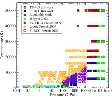
Figure 1 displays the pressure P and temperature T values at which ab initio simulations were performed. We have also included sample points from the IAPWS free energy formula-tion (Wagner & Pruß 2002) for completeness. For the internal energy and pressure, we found a good agreement between our calculations and the previous results ofFrench et al.(2009). We have therefore directly included these points in our ab initio set.
0.01 0.1 1 10 100 1000 10000 1e+05 1e+06 Pressure (GPa) 0 10000 20000 30000 40000 50000 Temperature (K) TF-MD this work SI-BCC this work Liquid this work Wagner 2002 Ice VII+X French 2009 Liquid French 2009 SI-BCC-French 2009
Fig. 1.Phase diagram of dense water obtained using the ab initio and
Thomas-Fermi simulations. Each symbol represents a simulation point. The phase state is indicated by a colored symbol according to the legend. Previous ab initio points obtained byFrench et al.(2009) as well as representative points ofWagner & Pruß(2002) are also shown. Figure1also shows that a superionic phase remains stable up to the highest pressures for temperatures up to 16 000 K.
The superionic phase is identified in our molecular dynamics simulations by looking at the mean square displacement of the hydrogen and oxygen ions as a function of time. Figure1shows that at ρ > 15 g cm−3the superionic phase remains stable up to
T = 16 000 K when considering either the BCC or FCC struc-tures. With the temperature grid used here, this suggests that the superionic-plasma phase boundaries for both the BCC and FCC structures vary slowly in this pressure range and are both located between 16 000 and 20 000 K. We also point out that the simu-lations performed here do not allow us to identify the superionic phase that is the most stable in this thermodynamic regime; nor do they indicate whether or not another superionic phase exists in this thermodynamical range.
Here, we do not further explore the exact determination of either the superionic-plasma boundary or the nature of the superionic state. The results previously obtained at low pres-sures indicated that this issue has little consequence for the EOS (French et al. 2016). To confirm that this remains the case for the entire density range considered here, we show in Table 1 the results obtained for the internal energy and pressure at rep-resentative densities and considering both the BCC and FCC superionic states. We see in Table1that the pressure and internal energy values agree to within 1.5%. We thus started our simula-tions with the BCC superionic lattice at ρ > 20 g cm−3, as this
enables smaller simulation cells. Using larger simulation cells, we verified that convergence is reached for pressure and internal energy up to 50 g cm−3.
2.3. Thomas-Fermi extension
Beyond 50 g cm−3, we switch from full ab initio simulations
to Thomas-Fermi molecular dynamics (TFMD) simulations
(Lambert et al. 2006). This consists in using the
Thomas-Fermi approximation to describe the electrons while propagating the ions on the resulting Born-Oppenheimer surface. In this
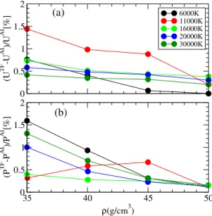
framework, the kinetic energy operator in the electronic Hamil-tonian is replaced by a functional of the density (Martins 2004). This greatly simplifies the calculation, as a plane wave basis is no longer needed and the electronic density is obtained by simply solving the Poisson equation. This represents the natural high-density limit to the DFT and hence to the ab initio simula-tions. Figure2shows the relative difference for the pressure P and internal energy U between the full ab initio and the TFMD simulations at densities between 34 and 50 g cm−3. For both
quantities, we see that the difference between the two methods is rapidly reducing as the density increases to be well under 1% at 50 g cm−3. This result clearly shows that the high-density limit is
reached and justifies the use of the Thomas-Fermi approximation beyond this density.
We further point out that the Thomas-Fermi approximation requires the use of a regularization potential. We make the choice of using the pseudopotential determined at ρ = 75 g cm−3 and
T = 2000 K throughout the entire range of interest. This approx-imation introduces an uncertainty on the internal energy of a few percent as the regularization formally breaks the transferability of the pseudopotential in density and temperature (Lambert et al. 2006). The internal energy obtained by the TFMD method is adjusted to the ab initio one at ρ = 50 g cm−3and T = 6000 K.
While the simulations were all started in the FCC phase, we make the choice of not recording the stability of the superionic phase as quantum effects for the protons may start to play a non-negligible role in its stability (French et al. 2016); the effect on the pressure and internal energy is a higher order effect.
3. Analytical fit of the Helmholtz free energy
The full ab initio simulation results presented in the previous sec-tion were used to construct a funcsec-tional form of the Helmholtz free energy valid over the entire density-temperature domain rel-evant to planetary modeling. Such an analytical fit of the free energy provides a convenient means to combine various data for use in simulations of interior structure or evolution of planets. For water, this includes the ab initio results presented above, valid down to a few gigapascals, and the low-energy IAPWS for-mulation (Wagner & Pruß 2002) that provides the EOS of water at P < 1 GPa in the vapor and liquid phases as constrained by experimental measurements.
3.1. Formulation
The parametrization of the Helmholtz free energy is expressed as
F = Ftran+ w(ρ, T)Flow+[1 − w(ρ, T)]Fhigh+FT− S0T, (1)
where each term has its own physical meaning. The first term,
Ftran=NH2OkBThln(nH2Oλ3H2O) − 1i , (2)
is the translational (ideal molecular gas) contribution. Here, NH2O=nH2OV = Nat/3 is the number of H2O molecules, Nat= natV = 3ρV/mH2Ois the total number of H and O atomic nuclei
in volume V, mH2O=2mH+mO=2.99 × 10⁻²³g is the mass of the molecule, kBis the Boltzmann constant, and
λH2O= 2π~ 2
mH2OkBT
!1/2
Table 1. Pressure PBCC and internal energy UBCC obtained for the BCC superionic phase and the differences ∆P = PFCC− PBCC and ∆U =
UFCC− UBCCbetween the FCC and BCC superionic phases, as well as fractional differences.
ρ(g cm−3) T (K) PBCC(Mbar) ∆P (Mbar) ∆P/P UBCC(eV atom−1) ∆U (eV atom−1) |∆U/U| (%)
7 6000 14.85 0.22 1.5% −685.9 0.03 0.004
15 6000 90.14 1.13 1.3% −668.7 0.52 0.08
20 6000 166.80 1.47 0.9% −656.5 0.66 0.10
25 6000 267.63 1.91 0.7% −643.5 0.76 0.12
40 11 000 709.97 0.9 0.13% −601 1.0 0.17
Notes. The reference energy corresponds to the total binding energy of the ground state of an isolated water molecule (693.3 eV atom−1).
0 0.5 1 1.5 2 (U TF -U AI )/U AI [%] 6000K 11000K 16000K 20000K 30000K 35 40 45 50 ρ(g/cm3) 0 0.5 1 1.5 2 (P TF -P AI )/P AI [%] (a) (b)
Fig. 2.Panel a: relative difference between the ab initio and
Thomas-Fermi internal energies as a function of density. Panel b: as in panel a but for the pressures.
is the thermal wavelength of a molecule. In the second and third terms of Eq. (1), Flow = N2 H2O V (bvdWkBT − avdW) +2 3NH2OkBT (bvdWnH2O)3/2[1 + (390.92 K/T)2.384] (4) and Fhigh(Nat,T, V) = Fe(NatZ∗,T, V) (5)
are the analytical expressions for the excess free energy in the moderate-density liquid regime (i.e., at ρ . 1 g cm−3 and
300 K . T . 2000 K) and at high densities (ρ 1 g cm−3),
respectively, which, together with Ftran, provide the fit to the
pressure as a function of density through the thermodynamic relation
P = −(∂F/∂V)T. (6)
Furthermore,
w(ρ, T) = 1
1 + (ρ/2.5 g cm−3+T/3509 K)4 (7)
is an interpolating function, which varies from 0 to 1 and ensures fitting the pressure as a function of density in the entire ρ − T
domain considered. In Eq. (5), Fe(Ne,T, V) is the Helmholtz
free energy of the ideal nonrelativistic Fermi gas of Ne =neV
electrons at temperature T, and Z∗is an effective charge number,
which is expressed as an analytical fitting function so as to adjust the pressure derived through Eq. (6) to the pressure data from the ab initio calculations. Explicitly,
Fe(Ne,T, V) = µeNe− P(e)id V, (8) where P(e)id = 8 3√π kBT λ3e I3/2(µe/kBT) (9)
is the effective (ideal Fermi gas) electron pressure, λe =
(2π~2/m
ekBT)1/2is the electron thermal wavelength,
µe=kBT X1/2(neλ3e√π/4) (10)
is the effective electron chemical potential, and Z∗= 103 1 + 2.35 rs 1 + 0.09/(rs√Γe) + 5.9 r 3.78 s (1 + 17/Γe)3/2 !−1 . (11) In Eq. (9), Iν(X) ≡ Z ∞ 0 xνdx exp(x − X) + 1 (12)
is the standard Fermi integral, and Xν(I) in Eq. (10) is the
inverse function. For both Iν(X) and Xν(I) we use the
Padé-type approximations of Antia (1993). In Eq. (11), Γe and rs
are the usual electron Coulomb parameter and density param-eter, respectively: Γe=e2/(aekBT) in the CGS system, and rs=
ae/a0,where ae=(43πne)−1/3is the electron-sphere radius, and
ne =10 nH2O is the total number density of all electrons (free
and bound). In Eq. (4), avdWand bvdWare the van der Waals
con-stants (respectively, 5.524 × 10¹²erg cm3mol−2and 30.413 cm3
mol−1; Grigoriev & Meilikhov 1997). The first line in Eq. (4)
reproduces the van der Waals EOS, which is sufficiently accu-rate at ρ 1 g cm−3, and the second line adjusts the EOS at
ρ∼ 1 g cm−3.
The fourth term in Eq. (1) reads
FT =−Nathb1τln(1 + τ−2) + b2τarctan τ + b3i
+NatkBT ln[1 + (0.019τ)−5/2], (13)
where b1 =3 × 10⁻¹³ erg, b2 =1.35 × 10⁻¹³ erg, b3 =2.43 ×
10−13 erg, and τ = T/Tcrit =T/647 K. It is derived from the
fitting correction to the residual internal energy, UT =Nat2b1τ− b2τ
2
1 + τ2 − b3Nat+
2.5NatkBT
This correction does not affect pressure but improves the fit to the internal energy, through the thermodynamic relation U = −T2 ∂ ∂T F T V . (15)
We note that we measure the total internal energy from its mini-mum at the ground state of the molecular phase so that U > 0 at any ρ and T. This definition is the same as in Wagner & Pruß(2002) but differs from the definition adopted in Table1 and Fig.2by the ground-state energy value of 11.14 MJ g−1. It
also differs by a constant of 77 kJ g−1 from the internal energy
given in French et al. (2009), French & Redmer (2015), and Soubiran & Militzer(2015).
The last term in Eq. (1), −S0T is an additional correction,
which affects neither P nor U, but shifts the entropy,
S = − (∂F/∂T)V, (16)
by constant S0. We find that the value S0 =4.9kBNatprovides the
best fit (within 10%) to the results presented for S bySoubiran & Militzer(2015) at ρ ≈ (1–2.5) g cm−3and T = (1000–6000) K.
However, entropy evaluation from our present fit should be used with caution especially when crossing the boundaries of different phases, where one can expect a discontinuity. This may lead to a value of S0that differs from one phase to the other.
The present analytical fit describes the EOS of liquid water at ρ.1 g cm−3and T . 2000 K, as well as plasma at 1 g cm−3.
ρ.102 g cm−3 and 103K . T . ×105 K. While not
includ-ing the super-ionic phase as a different phase, the sinclud-ingle-phase approximation used here provides a satisfactory description of the thermodynamical properties in this super-ionic regime. It has, however, a limited applicability for the ice VII and ice X phases that occur at T . 2000 K in the range (0.02–0.5) Mbar . P . 3 Mbar (Petrenko & Whitworth 1999). We also point out that quantum effects for the ions, which could be relevant at the highest densities and for low temperatures, are not included in the current parametrization. To build a fully multi-phase EOS for water, one can supplement our fit by the parametrizations con-structed specifically for the ice and super-ionic phases (French &
Redmer 2015; French et al. 2016). This will be the topic of
future work. Finally, we also point out that our analytical fit is less reliable in the domain of thermal ionization and dissocia-tion of molecular water, where ρ 1 g cm−3 and T 103K.
This regime is indeed poorly constrained by either the ab initio simulations or the IAPWS parametrization.
3.2. Validation of the analytical fit
We first verify the ability of the analytical fit to reproduce both the results of theoretical calculations and the IAPWS free energy model. In Figs.3 and4, we compare the behavior of pressure and internal energy obtained with the input data at low and high densities and temperatures, respectively.
As we are primarily interested in planetary interiors, the accurate description of the liquid-vapor transition below the crit-ical point located at Tcrit =647 K and Pcrit =22.064 MPa is
beyond the scope of this study. Furthermore, these conditions are tied to an accurate modeling of the atmosphere of the planet that do not directly involve an EOS such as the one developed here. Figures 3a and b suggest that without atmospheric treat-ment, interior models should consider the liquid state for surface conditions when the surface temperature is below the critical point. We expand on this point in the following sections.
Fig. 3. Comparison between the input data and the analytical fitted
isotherms for the pressure P (panel a) and for the internal energy U (panel b) at relatively low densities. Symbols show the data: the IAPWS
(Wagner & Pruß 2002) published table for P < 1 GPa (straight crosses)
and extension to P > 1 GPa according to the IAPWS free-energy model (squares); results of ab initio calculations bySoubiran & Militzer(2015; empty diamonds) and byFrench et al.(2009; oblique crosses for liq-uid, inverted triangles for ice X, filled diamonds for the superionic [SI] phase). Solid lines represent the present fit; dotted lines represent the fit
ofFrench & Redmer(2015) for ice X.
At the lowest densities, we see in Fig.3a that the pressure turns negative along the 300 and 600 K isotherms for densi-ties below 1 g cm−3. Figure3b indicates that this translates to a
minimum for the internal energy. This corresponds to the cross-ing of the liquid–vapor phase boundary and a region where the pressures are formally negative, which in fact corresponds to phase coexistence. For instance, for the 300 K isotherm the ana-lytical fit gives a region of negative pressures expanding from 0.9 to 0.1 g cm−3. We note that the IAPWS data (Wagner &
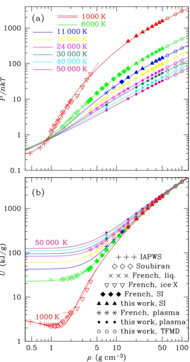
Fig. 4.Comparison of the data with the analytical fitted isotherms at high densities for the pressure normalized to the ideal atomic gas value, P/natkBT (panel a), and for the internal energy U (panel b).
Sym-bols show the data: the IAPWS table (Wagner & Pruß 2002, straight crosses); results of ab initio calculations bySoubiran & Militzer(2015; empty diamonds); ab initio calculations byFrench et al.(2009; oblique crosses for liquid, inverted triangles for ice X, filled diamonds for the superionic [SI] phase, asterisks for the plasma phase); and the results of our present ab initio calculations (filled triangles for the SI phase and filled dots for the plasma phase), supplemented with our TFMD calcula-tions at ρ > 50 g cm−3(empty circles). Solid lines represent the present
fit; the dotted line represents the fit ofFrench & Redmer(2015) for ice X at T = 1000 K.
density of ∼10−3 g cm−3 on this isotherm. The agreement
improves for the 600 K isotherm. We see that the analytical fit reproduces the overall behavior of the pressure across the liquid-vapor boundary. However, it extends this boundary to a higher temperature, giving the critical point at 683 K and 0.331 g cm−3
(to be compared with the experimental values of 647 K and 0.322 g cm−3).
Figures3a and b also indicate that the agreement with the ab initio data at higher temperatures is satisfactory up to 6000 K. We note that the ab initio results and the free energy model pre-dictions are not in perfect agreement at 1000 K. As the ab initio method becomes less reliable as density decreases, mainly due to the deficiency of density functional theory in under-dense regime, the ab initio results fail to match the IAPWS formula-tion at low density. Our analytical fit eliminates this mismatch by interpolation between the low-density IAPWS and high-density ab initio data.
Figures4a and b show the data and fitted isotherms for the pressure and internal energy across the entire density range at higher temperatures, 1000 K ≤ T ≤ 50 000 K. Figure4a displays the pressure normalized to the atomic ideal gas contribution natkBT. As noted above, the fit does not perfectly reproduce the
ab initio data for the ice X phase along the 1000 K isotherm at 2.5 g cm−3≤ ρ ≤ 4 g cm−3. However, it satisfactorily reproduces
the thermodynamical properties, despite the fact that the system crosses a number of various phases in the ρ–T domain displayed in the figures.
We also point out that the data represented in Figs.3and4by empty symbols (the ice phase, the data bySoubiran & Militzer 2015, and the Thomas-Fermi results) have not been explicitly included to construct the analytical fit. We see that the data by Soubiran & Militzer(2015) is in good agreement with the pre-diction of the analytical fit. Furthermore, the good agreement found with the Thomas-Fermi results up to 100 g cm−3 shows
the validity of the analytical fit up to this high density.
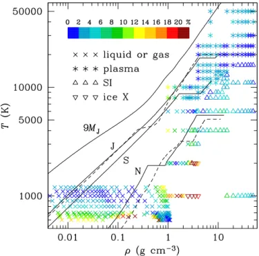
Figures 5 summarizes the applicability of the current analytical EOS for planetary modeling. We display the accuracy of the analytical fit as a color code corresponding to the residual difference between the predicted and input P and U values. On the same figure, we also show representative interior profiles for Jupiter, Saturn, and Neptune that display a significant amount of water in their interior. This shows that the analytical fit is accurate for modeling these objects. For comparison, the profile of a 9MJplanet is also shown. As pointed out before, the
single-phase approximation used for this analytical fit ignores the discontinuities due to the phase changes between the different phase states. For the phase transition between the liquid state and ice X, the discrepancies increase to tens of percent. Otherwise we see that the fit remains a reasonable approximation for both the pressure and internal energy throughout the relevant thermodynamical domain.
4. Comparison with experimental data and previous EOSs
We now turn to compare the predictions of the analytical fit developed in Sect.3 with existing experimental data from both static and dynamical experiments. We compare these predic-tions with EOSs commonly used in planetary interior models. In Fig.6, we compare the predictions of the analytical fit devel-oped with the static high-pressure data obtained using diamond anvil cells (Hemley et al. 1987;Sugimura et al. 2008). We also show in Fig.6the 1000 K isotherm and its corresponding ab ini-tio data to further illustrate the approximaini-tion made by not accounting explicitly for the solid ice phases and extending the liquid throughout the solid phases. We see that the analytical fit thus misses the jump between the liquid and ice X phases at ρ ∼ 2.5 g cm−3, as we have already seen in Fig.4.
The T = 300 K isotherm behaves similarly. We see that both the IAPWS free energy formulation and our analytical fit, being
Fig. 5. Points in the ρ–T plane where the input data have been used to construct the analytical fit. Different symbols correspond to different phase states: crosses for liquid, asterisks for plasma, upright triangles for superionic state, and reverted triangles for ice X. The colors of the symbols represent the accuracy of the fit (for both P and U, i.e., the maximum of the two residuals) according to the palette above the leg-end. The lines show isentropes of Jupiter (J), according to the models of
Leconte & Chabrier(2012) andNettelmann et al.(2012; the solid and
dashed lines, respectively), Saturn (S), according toLeconte & Chabrier
(2012), Neptune (N) according to two models ofNettelmann et al.(2013; solid and dashed lines), and a planet with M = 9 MJ(seeBaraffe et al.
2008,2010).
continued from the low-density region at T = 300 K, overesti-mate the pressure (underestioveresti-mate the density) in the ice phases at higher densities. At P = 10 GPa, the resulting density is about 7% lower than in the ice phases. This should be compared with the predictions ofSeager et al.(2007) who used T = 0 K DFT calculations for the various ice phases to construct their EOS. By neglecting the effect of temperature and the phonon contri-bution, they overestimate the density of dense water by about 3% at 10 GPa. We also note that this difference with the experimen-tal data tends to decrease as the pressure increases for both EOSs. Therefore, the most significant difference resulting from neglect-ing the ice phases that we can anticipate for interior structure calculations could be for the pressure profile of the outer layer of a planet, if it had T ∼ 103 K at ρ ∼ 3 g cm−3. From Fig.5we
see that this is not the case for the giant planets, for which the temperature is much higher and therefore the temperature profile passes well above this phase jump.
We also point out some differences between the two ab initio calculations beyond 4 g cm−3. We attribute these differences to
the use of different functionals in the Thomas-Fermi approxima-tion; we further investigate their impact on the interior structure models in the following sections.
Figure 7 shows a comparison between the predictions of our analytical fit deduced from ab initio simulations and the measured experimental data along the principal shock Hugo-niot line. For a given initial state, the Rankine-HugoHugo-niot relation determines the final states allowed by conservation of energy and momentum during a shock. It is directly related to the
1.5 2 2.5 3 3.5 4 4.5
ρ(g/cm
3)
1 10 100
Pressure (GPa)
Hemley et al. 1987Seager et al. 2007 Sugimura et al. 2008 Ab initio 1000K IAPWS-95 Fit T=300K Fit T=1000K
Fig. 6.Comparison of the analytical fit predictions with high-pressure
data at T = 300 K. EOS and reads
U − U0= P + P2 0(V0− V), (17)
where subscript 0 indicates the initial state. The principal Hugo-niot corresponds to a single shock, obtained with initial state at rest in normal conditions. Figure7 shows that shock exper-iments probe a range of pressures almost an order of magnitude higher than when using diamond anvil cells (Fig.6). This also corresponds to a significant increase in temperature. The temper-ature reaches about 5000 K around 100 GPa for a shock, while it remains near 300 K in diamond anvil cell experiments. With the increase of the shock pressure beyond 500 GPa, the temperature exceeds 50 000 K. Since the input ab initio data that underlie our fit have been obtained for T ≤ 50 000 K, the accuracy of the fit at higher temperatures is not guaranteed (the corresponding part of the Hugoniot line is drawn by long dashes in Fig.7).
Figure7shows a good agreement at low pressures with early data obtained using explosion (Volkov et al. 1980) and gas-gun techniques (Mitchell & Nellis 1982;Lyzenga et al. 1982). The unique measurement of the water EOS at P > 1000 GPa, published long ago by Podurets et al. (1972), is satisfacto-rily described by the above-mentioned continuation of our fit beyond the range where it has been constrained by the data. The first laser shock data obtained in the 100–1000 GPa range by Celliers et al. (2004) are much softer than the analytical fit. This experimental data set is in good agreement with SESAME 7150 predictions. In contrast, we see that the analytical fit agrees very nicely with the more recent experimental data ofKnudson et al. (2012) obtained using the Z-pinch techniques, as well as with the latest results of Kimura et al. (2015). This confirms that earlier laser shock experiments likely suffer from system-atic errors which could be caused by the standard used in the impedance-matching method (Knudson & Desjarlais 2009). This experimental set is therefore not considered here to validate the behavior of water at high pressures and temperatures. This also highlights that the SESAME 7150 predictions, which are in good agreement with the data ofCelliers et al.(2004), should be ruled
Fig. 7. Principal Hugoniot line in the ρ–P plane calculated using the present fit (solid line for T < 50 000 K, continued by long-dashed line for T > 50 000 K) compared with experimental data (dots with error bars) ofPodurets et al.(1972; as reanalyzed byKnudson et al. 2012; the original result ofPodurets et al. 1972is also shown with dotted error bars), Volkov et al.(1980); Mitchell & Nellis(1982);Lyzenga et al.
(1982);Celliers et al.(2004);Knudson et al.(2012), andKimura et al.
(2015). For comparison, the principal Hugoniot lines predicted by the SESAME (Lyon & Johnson 1992) and ANEOS (Thomson & Lauson 1972) models are shown by the dotted line and short-dashed line, respec-tively. Inset panel: principal Hugoniot line in the ρ–T plane calculated from the fit and the experimental data points fromLyzenga et al.(1982)
andKimura et al.(2015).
out for planetary modeling. The SESAME 7150 model is not considered a reliable EOS nowadays, but it is still in use for plan-etary modeling (Miguel et al. 2016). This is also the case for the ANEOS model (Thomson & Lauson 1972). Figure7shows that ANEOS predictions depart from the data ofKnudson et al. (2012) at ρ > 2.5 g cm−3significantly outside the experimental
error bars.
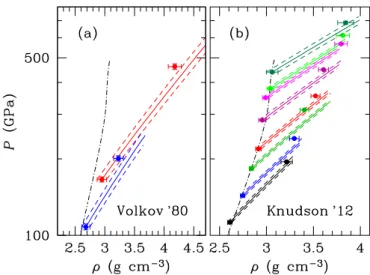
Figure8shows a comparison between the predictions of our analytical fit and the EOS measurements obtained using double-shock experiments (Volkov et al. 1980; Knudson et al. 2012), where the initial shock wave is reflected from a surface of a stan-dard material (aluminum or quartz). In this case, the initial state in Eq. (17) lies on the principal Hugoniot line and represents the initial condition for the secondary Hugoniot. Since the latter ini-tial condition is measured with some uncertainties, the position of the secondary Hugoniot is not firmly defined. We therefore show the 1σ limits for each secondary Hugoniot that arise from these uncertainties in the initial state.
Figure9shows a comparison between the predictions of our analytical fit with two EOS measurements in experiments using laser-induced shock in statically compressed water. We find a better agreement with the latest dataset ofKimura et al.(2015) compared to that ofLee et al.(2006). We show these for com-pleteness as the scatter in the experimental data cannot further constrain the validity of the analytical fit.
Overall, we find that our present analytical fit provides a satisfactory description of both the static and dynamical experimental results available to date for dense water. We now
Fig. 8.Comparison of experimental data for reshocked water (points
with error bars) with corresponding Hugoniot lines calculated from the analytical fit (solid lines). The principal Hugoniot is shown by the dot-dashed line. Dashed lines show the theoretical regions defined by taking into account 1σ experimental uncertainties for the initial (primary-shock) states. Panels a and b: comparison for the data ofVolkov et al.
(1980) and ofKnudson et al.(2012), respectively.
Fig. 9. Comparison between the calculations based on our analytical
fit and the experimental shock data for initially precompressed water. Panel a: points measured byLee et al.(2006). Panel b: points obtained
by Knudson et al.(2012). The inset in each panel shows the initial
pressures and densities measured.
turn to illustrate the applications of the EOS developed for the interior structure of different classes of planets.
5. Implication for planetary interiors
The internal structure calculations are performed by solving the standard hydrostatic, mass, and energy conservation equations
(e.g.,Schwarzschild 1958;Kippenhahn et al. 2012), ∂P ∂r =−ρg, (18) ∂T ∂r = ∂P ∂r T P ∇T, (19) ∂m ∂r =4πr2ρ, (20)
where P is the pressure, ρ the density, g = Gm/r2 the gravity,
G is the gravitational constant, m is the mass enclosed within a sphere of radius r, and ∇T =d ln T/d ln P depends on the mechanism of energy transport. If the medium is stable against convection, then ∇T = 3 16 PK g T4 eff T4, (21)
where Teff is the effective surface temperature and K is the
effective opacity. If the transport of energy is dominated by convection, then in the simplest (Schwarzschild) approximation ∇T =∇ad, where ∇ad= ∂∂ln Tln P S (22)
is the adiabatic gradient.
The interior structure of a planet of a given mass, M, is obtained by integrating inward the set of Eqs. (18)–(20), starting from a boundary condition defined by a fixed surface temper-ature and pressure. This is formally given by either in situ measurements for planets of the solar system or full atmospheric calculations for exoplanets. As we are primarily interested in test-ing our EOS for dense water, we devise strategies to overcome this difficulty for each type of planet that we consider.
5.1. Water planets
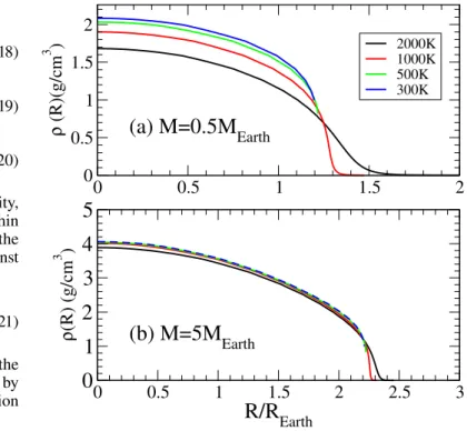
In order to test the accuracy of our EOS, we first turn to the calculation of the inner structure and mass-radius relationship of a planet entirely made of water. This is a purely academic exercise disconnected from the outcomes of planetary formation but the resulting mass-radius relationship remains a well-used benchmark to classify exoplanets (Seager et al. 2007). It also allows us to decipher the influence of temperature on both the inner structure and mass-radius relationship. Figure 10 shows the effect of temperature on isothermal interior structure mod-els for planets of 0.5 and 5 MEarth, respectively. In this situation,
the temperature throughout the planet is constant and equal to the surface temperature, Tsurf. The outer boundary conditions are
chosen as 1 bar for temperature above the critical point and at the liquid-vapor boundary below. This corresponds to different sur-face densities and close to 1 g cm−3for the two models using a
surface temperature below the critical value.
Figure10 shows that within this model, the effect of tem-perature is twofold. As the EOS developed fully accounts for temperature throughout the density range covered by the con-ditions existing in planetary interiors, it affects the extent of the outer edge boundary as well as the compressibility deeper within the planet. Figure 10 shows that both these effects are impor-tant for low-mass planets where we notice a radius increasing by a factor of two when the surface temperature varies from 300 to 2000 K. This increase in radius comes from a significant
0
0.5
1
1.5
2
0
0.5
1
1.5
2
ρ
(R)(g/cm
3)
2000K 1000K 500K 300K0
0.5
1
1.5
2
2.5
3
R/R
Earth0
1
2
3
4
5
ρ
(R) (g/cm
3)
(a) M=0.5M
Earth(b) M=5M
EarthFig. 10. Isothermal density profiles of pure-water planets for varying
surface temperatures. The values of the surface temperature, Tsurf, are
indicated in the figure for a planet of mass M = 0.5 MEarth(panel a) and
for a planet of mass M = 5 MEarth (panel b). REarth is the radius of the
Earth.
expansion of the low-density outer edge beyond 1.5 REarth that
follows the rapid expansion of the supercritical liquid at high temperatures and low surface gravity. It also comes from the sig-nificant temperature dependence of the water EOS for densities below 2 g cm−3previously pointed out in Fig.6. For a planet of
0.5 MEarth, the maximum pressure reached at the center of the
planet is 0.18 Mbar for a temperature of 2000 K and 0.27 Mbar for a temperature of 300 K.
Figure10shows that the effect of temperature decreases sig-nificantly when the planet size increases. This comes from both a smaller expansion of the outer edge resulting from a larger surface gravity, and a reduced temperature dependence of the EOS as the density increases. Figure10shows that the density profile of the planet is dominated by densities between 2 and 4 g cm−3for a planet of 5 MEarth. Figure6shows that the
temper-ature dependence of the EOS is almost negligible in this density range. The effect of temperature is therefore reduced to a small expansion of the outer edge that leads to an increase of 10% of the radius. This suggests that the effect of temperature becomes negligible as the mass of the planet increases.
Figures11a and b give the mass-radius relationship obtained with the current EOS and calculated for the complete range of planets detected to date, and a zoom for planets below 10 MEarth
(Exoplanet Team 2018). As anticipated above, we see that the
temperature dependence decreases as the mass of the planet increases. Figure11b shows that the temperature effect is rather important for planets smaller than 10 MEarth. We also see in
Fig.11a that the temperature dependence for pure-water planets can be neglected for planets larger than 15 MEarthwhen
consid-ering an isothermal temperature profile. We also find that the mass–radius relationship obtained with the EOS developed in the current work is consistent with the calculations ofSeager et al.(2007) for the entire range of planets detected. Figures11a
1 10 100 1000 10000 M/MEarth 1 10 R/R Earth
Tsurf=250K, Psurf=1bar Tsurf=2000K, Psurf=1bar Seager 2007 (a) 0 2 4 6 8 10
M/M
Earth 0.5 1 1.5 2 2.5 3R/R
Earth Seager 2007Tsurf=250K, Psurf=100kbar Tsurf=250K, Psurf =1bar Tsurf=2000K, Psurf=1bar
Kepler-10b CoroT-7b Kepler-138b 55 Cnc e Kepler-18b Kepler-307c Kepler-11b Kepler-11f GJ1214b Earth 100% H20 100% Fe 100%MgSiO3 Kepler-80c
(b)
Fig. 11.Mass-radius relationship for pure-water planets in an isothermal
model. The surface temperature and pressure are indicated in the figure and compared to the result ofSeager et al.(2007) over the entire range of planets currently detected (panel a); for planets with mass less than 10 MEarth(panel b). Isothermal models for pure silicates (MgSiO3) and
iron (Fe) (Bouchet et al. 2013;Mazevet et al. 2015) are also displayed. and b show that the radius obtained with the EOS developed here and for an isothermal model with surface temperature of 250 K is 3% higher than the results ofSeager et al.(2007) for planets less than 10 MEarthand 2% lower above this planetary mass. This
latter result comes from the difference in the behavior of the two EOS at high densities already mentioned in the previous sec-tion. For low-mass planets, where inspection of Fig.7indicates the largest difference between the EOS developed here with both the experimental data and the zero temperature EOS ofSeager et al.(2007), we also find a rather satisfactory agreement. This indicates that neglecting the ice phases has a minimal impact on the resulting mass–radius relationship even for low-mass plan-ets. For benchmarking purposes, we also show in Fig.11b that the zero temperature results ofSeager et al.(2007) can be recov-ered with the current EOS by considering a surface pressure of 10 GPa (0.1 Mbar). 0 2 4 6 8 10
M/M
Earth 0.5 1 1.5 2 2.5 3R/R
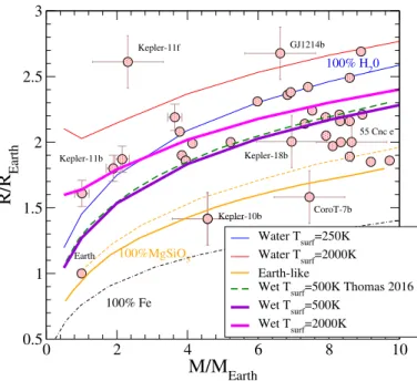
Earth Water Tsurf=250K Water Tsurf=2000K Earth-likeWet Tsurf=500K Thomas 2016 Wet Tsurf=500K Wet Tsurf=2000K Kepler-10b CoroT-7b Kepler-11b 55 Cnc e Kepler-18b Kepler-11f GJ1214b Earth 100% H20 100% Fe 100%MgSiO3
Fig. 12.Temperature dependence of the mass–radius relationship for
isothermal models of wet super-Earth planets containing 50% water denoted as Wet. The surface temperatures are indicated in the figure. The dots represent detected planets in this range of planetary mass. Isothermal models: pure water (water), silicates (MgSiO3), iron (Fe),
Earth-like composition containing 66% silicates and 33% iron (Earth-like;Bouchet et al. 2013;Mazevet et al. 2015). The benchmark calcu-lations for wet super-Earth planets are fromThomas & Madhusudhan
(2016).
Finally, we notice in Fig.11b that several detected planets fall within the temperature-dependent range of the isothermal pure-water model. This suggests that temperature-dependent effect on the mass-radius relationship needs to be included when consid-ering the interior structure to identify the nature of these objects. We pursue further this suggestion using more realistic interior structure models and by considering wet super-Earths and ocean planets.
5.2. Wet super-Earth planets or ocean planets
Wet super-Earth or ocean planets are objects that have no equiv-alent in the solar system. They have been introduced to interpret the continuum of planets detected between pure water and Earth-like object. Earth-Earth-like planets consist of objects of varying mass but following the Earth composition (33% Fe, 66% MgSiO3by
mass). Wet Super-Earths consist of an Earth-like core made of 33% iron and 66% silicates and a significant fraction of water outside the core (Valencia et al. 2006;Thomas & Madhusudhan 2016). To test the validity of our EOS at describing these objects, we show in Fig. 13 the mass–radius relationship obtained by considering isothermal models and wet super-Earth planets con-stituted of 50% water. The iron and silicates EOSs used are tem-perature dependent and, similarly to the water EOS developed here, are described by free-energy functional forms adjusted directly to ab initio calculations (Bouchet et al. 2013;Mazevet et al. 2015).
Figure12shows the mass–radius relationship for isothermal models obtained using two different surface temperatures. For a surface temperature of Tsurf=500 K, we obtained a rather
satis-factory agreement with the previous calculations ofThomas &
0 2 4 6 8 10
M/M
Earth 0.5 1 1.5 2 2.5 3R/R
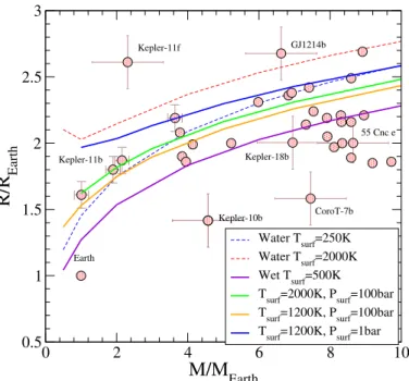
Earth Water Tsurf=250K Water Tsurf=2000K Wet T surf=500KTsurf=2000K, Psurf=100bar Tsurf=1200K, Psurf=100bar Tsurf=1200K, Psurf=1bar
Kepler-10b CoroT-7b Kepler-11b 55 Cnc e Kepler-18b Kepler-11f GJ1214b Earth ect of temperature on the mass-radius relationship beyond the simple isothermal model where the temperature is kept constant throughout the planet.
Fig. 13.Temperature dependence of the mass–radius relationship for
adiabatic models of wet super-Earth planets containing 50% water as solid lines. The surface temperatures and pressures are indicated in the figure. The dots represent detected planets in this range of plane-tary mass. The isothermal models for pure-water planets (dashed) and wet super-Earth planets (purple) with the corresponding surface tem-peratures are also displayed in the figure. These correspond to the data shown in Figs.11and12, respectively.
condition used in the current work follows a somewhat different prescription. As mentioned before, we do not consider the vapor phase for surface temperature below the critical point and use the liquid-vapor boundary at 1 bar as outer boundary conditions. Figure12shows that the temperature dependence of the mass– radius relationship is rather significant and cannot be neglected when assessing the interior structure of these objects, in agree-ment with the conclusions ofBaraffe et al.(2008). Indeed, we see in Fig. 12 that several planets lie between the boundaries delimited by the two surface temperatures. As for the case of the pure water planets, the temperature dependence decreases as the mass of the planet increases and becomes negligible beyond 15 MEarth.
The wet Earth-like model that is 50% water is at a mid-point between the dry Earth-like planets and pure-water planets. By extension of the temperature dependence shown for plan-ets that are 50% water, we can anticipate that this also needs to be taken into account to deduce the composition of objects such as Kepler-18b or 55Cnc that hold a significant fraction of water themselves. In this case, the amount of water deduced will directly depend on the surface temperature considered. Along the same line of reasoning, we can also anticipate that the overlap between the pure water and wet Earth-like planet with a surface temperature of Tsurf =2000 K shown below 2 MEarthfor a
com-position of 50% water will expand to planets with larger mass when the fraction of water is increased. To make a more quanti-tative statement on this issue requires to go beyond the internal structure calculations and to account for an accurate modeling of the atmosphere as well as the amount of light received from the host star. Both these topics are beyond the scope of this study that aims at validating the EOS for dense water developed here. We instead turn to the evaluation of the effect of temperature on the
mass–radius relationship beyond the simple isothermal model where the temperature is kept constant throughout the planet.
The EOS developed in the current work provides the total entropy thanks to the parametrization of the Helmholtz free energy using the ab initio results. This allows us to calculate more realistic interior models by considering a water layer under-going nearly adiabatic convection. The uncertainty in defining S0 pointed out in Sect. 3 does not affect these results as long
as the convective layer remains within a single thermodynamic phase. The previous isothermal models and the adiabatic ones bracket the maximum impact of the water EOS upon the mechan-ical structure of the body. We see in Fig. 13that the effect of temperature on the mass–radius relationship is almost two times more important when considering the water layer as adiabatic rather than isothermal. When considering a surface pressure of 1 bar, Fig. 13 shows that the radius obtained up to 10 MEarth
is significantly larger than that in the pure-water case at zero temperature. This effect is the most spectacular for surface tem-perature above the critical temtem-perature. It remains limited when the surface temperature is below the critical point. We also point out that the surface pressure tends to reduce this effect. Figure13 shows that the radius decreases by 20% at 1200 K when the surface pressure increases from 1 to 100 bars. This suggests that neglecting the effect of temperature when identifying the internal structure of exoplanets leads to overestimatations of the overall amount of water, especially for objects close to their par-ent star and receiving a significant amount of light. This needs to be tempered by the probable escape of the atmosphere under these particular conditions and will need to be assessed on a case by case basis with a proper treatment of the atmosphere. 5.3. Core of giant planets
We now turn to the last situation where a temperature-dependent EOS for dense water is important for planetary modeling the core of giant planets. Following the well-accepted core-accretion scenario (Pollack et al. 1996), a significant amount of water is expected in the core of giant planets. This potentially significant amount of water stems from the likely composition of the initial core that triggered the accretion of a large fraction of hydro-gen and helium. The exact amount of water as well as the size of the core for a planet like Jupiter is a matter of debate and one of the main scientific goals of the Juno mission (Bolton et al. 2017). The probe is currently measuring Jupiter’s high-order gravitational moments for Jupiter to decipher the amount of metallic element present in the interior as well as their dis-tribution throughout the planet (Wahl et al. 2017). This goal requires an accurate modeling of the EOS for all the elements potentially constituting the planet, including water.
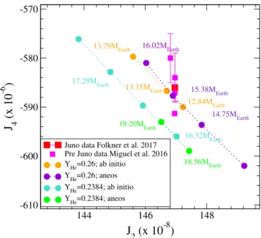
Figure14shows the dependence of Jupiter’s first two gravi-tational moments, J2and J4, on the dense water EOS used in the
modeling of the interior. Jupiter’s interior is obtained by solv-ing the standard hydrostatic equilibrium Eqs. (18)–(20) and by considering the planet as composed of an H-He envelope and a pure-water core (we note the assumption of a fully adiabatic inte-rior profile here). The hydrogen and helium EOSs used for the envelope are also based on ab initio simulation results (Caillabet et al. 2011;Soubiran 2012). The gravitational moments are cal-culated using the theory of figures to the third order (Zharkov & Trubitsyn 1978).
Figure 14 shows the values of the first two gravitational moments obtained using two different water EOSs, namely the present and the widely used ANEOS ones, to describe the core and by considering two different helium concentrations. The size
144 146 148
J
2(x 10
-8)
-610 -600 -590 -580 -570J
4(x 10
-6)
Juno data Folkner et al. 2017 Pre Juno data Miguel et al. 2016 YHe=0.26; ab initio YHe=0.26; aneos YHe=0.2384; ab initio YHe=0.2384; aneos 14.75MEarth 16.02MEarth 13.15MEarth 12.84MEarth 16.32MEarth 17.29MEarth 15.38MEarth 18.56MEarth 19.20MEarth 13.79MEarth erent compressibilities for pressures and temperatures relevant to Jupiter’s inner core. These conditions correspond to pressures above 40 Mbar and temperatures between 15 000 and 20 000 K depending on the hydrogen-helium EOSs used, Miguel et al. (2016). In this ther-modynamical region, the two water EOSs predict pressures that
di
Fig. 14.Dependence of Jupiter’s first two gravitational moments on the
dense-water EOS used, namely the present and ANEOS ones. The cal-culations are performed in a two-layer model for a fixed value of the mass fraction of He in the envelope, YHe, indicated in the graph where
the mass of the dense water core varies. The size of the pure water core is indicated for a few sample points in the figure. The pre-Juno values of the gravitational moments are the values collected inMiguel et al.
(2016) while the Juno data are fromFolkner et al.(2017).
of the core is varied to the values indicated in the graph. The first mass fraction of helium, YHe =0.2384, corresponds to the
Galileo measurements, while a slightly higher mass fraction, YHe =0.26, allows us to reproduce the values of the two
gravita-tional moments J2 and J4. Within a two-layer model of Jupiter,
the first case reproduces the observed radius of the planet as well as the value of J2 measured but, as shown in Fig.14, it misses
the J4moment by slightly more than 1%. Conversely, in the case
where the mass fraction of helium is increased to YHe =0.26, the observed radius is underestimated by slightly more than 1% while matching the first two gravitational moments. This short-coming of the two-layer model for Jupiter, namely a central core surrounded by a homogeneous gaseous envelope, has been well documented elsewhere (Miguel et al. 2016). We point out here that this issue is not resolved by using different water EOSs for the core.
We see in Fig.14that using different water EOSs leads to different predictions regarding the size of the core. These two predictions in the size of the core differ by close to 20%, and do not depend on the helium concentration. We note that this also translates into different average and maximum densities reached in the central core. The EOS developed here predicts a pure-water core density more than 25% higher than in the case of the widely used ANEOS one. The highest density reached in the former case is close to 12.45 g cm−3, while it remains close
to 9.67 g cm−3in the latter case. This difference is comparable
with the variation of the core density when a pure-ice core is replaced by a core of pure rock, as pointed out byGuillot(1999). In our case, this can be traced back to significant discrepancies between the two EOSs, which predict different compressibilities for pressures and temperatures relevant to Jupiter’s inner core. These conditions correspond to pressures above 40 Mbar and temperatures between 15 000 and 20 000 K depending on the
hydrogen-helium EOSs used,Miguel et al.(2016). In this ther-modynamical region, the two water EOSs predict pressures that differ by more than 10%. This shows that the current EOS is useful to accurately calculate the exact size of the core that is potentially present at the center of giant planets.
6. Summary
In summary, we developed an EOS for water applicable to the full range of thermodynamic conditions relevant to planetary modeling. This encompasses the range from outer layers of wet super-Earth to the core of giant planets. This EOS includes an evaluation of the entropy (within an arbitrary constant value S0,
Sect. 3, which can differ from one phase to another but has no impact on all other thermodynamic quantities) thanks to the parametrization of the Helmholtz free-energy functional form on the ab initio results. Using this EOS, we show that the temper-ature dependence of the EOS needs to be accounted for when analyzing the composition and nature of exoplanets using the standard mass–radius relationship, a point already stressed by Baraffe et al.(2008). We also show that an accurate description of the thermodynamic properties of dense water is required to deduce the mass of the core of giant planets from gravitational moments as it is currently measured for Jupiter by the Juno mis-sion. As discussed in Sect.3, the EOS developed here is not very accurate for the solid ice phases. This does not noticeably affect the planetary gross properties, such as the mass–radius relation-ship, but may produce an error of several percent in calculations of temperature profiles. To include explicitly all the ice phases as well as treating the super-ionic phase will be the topic of further development of the present EOS.
Acknowledgements. Part of this work was supported by the SNR grant PLAN-ETLAB 12-BS04-0015 and the Programme National de Planetologie (PNP) of CNRS-INSU co-funded by CNES. Funding and support from Paris Sciences et Lettres (PSL) university through the project origins and conditions for the emergence of life is also acknowledged. This work was performed using HPC resources from GENCI- TGCC (Grant 2017- A0030406113) and was granted access to the HPC resources of MesoPSL financed by the Region Ile de France and the project Equip@Meso (reference ANR-10-EQPX-29-01) of the pro-gramme Investissements d’Avenir supervised by the Agence Nationale pour la Recherche.
References
Antia, H. M. 1993,ApJS, 84, 101
Baraffe, I., Chabrier, G., & Barman, T. 2008,A&A, 482, 315
Baraffe, I., Chabrier, G., & Barman, T. 2010,Rep. Prog. Phys., 73, 016901
Becker, A., Lorenzen, W., Fortney, J. J., et al. 2014,ApJS, 215, 21
Benuzzi-Mounaix, A., Mazevet, S., Ravasio, A., et al. 2014,Phys. Scr., T161, 014060
Bolton, S. J., Adriani, A., Adumitroaie, V., et al. 2017,Science, 356, 821
Bouchet, J., Mazevet, S., Morard, G., Guyot, F., & Musella, R. 2013,
Phys. Rev. B, 87, 094102
Caillabet, L., Mazevet, S., & Loubeyre, P. 2011,Phys. Rev. B, 83, 094101
Cavazzoni, C., Chiarotti, G. L., Scandolo, S., et al. 1999,Science, 283, 44
Celliers, P. M., Collins, G. W., Hicks, D. G., et al. 2004,Phys. Plasmas, 11, L41
Exoplanet Team. 2018, The Extrasolar Planets Encyclopaedia, http://www. exoplanet.eu
Folkner, W. M., Iess, L., Anderson, J. D., et al. 2017,Geophys. Res. Lett., 44, 4694
French, M., & Redmer, R. 2015,Phys. Rev. B, 91, 014308
French, M., Mattsson, T. R., Nettelmann, N., & Redmer, R. 2009,Phys. Rev. B, 79, 054107
French, M., Desjarlais, M. P., & Redmer, R. 2016,Phys. Rev. E, 93, 022140
Gonze, X., Amadon, B., Anglade, P. M., et al. 2009,Comput. Phys. Commun., 180, 2582
Grigoriev, I. S., & Meilikhov, E. Z. 1997,Handbook of Physical Quantities(Boca Raton: CRC-Press)
Guillot, T. 1999,Planet. Space Sci., 47, 1183
Guillot, T., Miguel, Y., Militzer, B., et al. 2018,Nature, 555, 227
Hemley, R. J., Jephcoat, A. P., Mao, H. K., et al. 1987,Nature, 330, 737
Holzwarth, N. A. W., Tackett, A. R., & Matthews, G. E. 2001,Comput. Phys. Commun., 135, 329
Hubbard, W. B., & Militzer, B. 2016,ApJ, 820, 80
Jollet, F., Torrent, M., & Holzwarth, N. 2014,Comput. Phys. Commun., 185, 1246
Kimura, T., Ozaki, N., Sano, T., et al. 2015,J. Chem. Phys., 142, 164504
Kippenhahn, R., Weigert, A., & Weiss, A. 2012,Stellar Structure and Evolution, 2nd edn, Astronomy and Astrophysics Library (Berlin, Heidelberg: Springer) Knudson, M. D., & Desjarlais, M. P. 2009,Phys. Rev. Lett., 103, 091102
Knudson, M. D., Desjarlais, M. P., Lemke, R. W., et al. 2012,Phys. Rev. Lett., 108, 091102
Lambert, F., Clérouin, J., & Zérah, G. 2006,Phys. Rev. E, 73, 016403
Leconte, J., & Chabrier, G. 2012,A&A, 540, A20
Lee, K. K. M., Benedetti, L. R., Jeanloz, R., et al. 2006,J. Chem. Phys., 125, 014701
Lyon, S. P., & Johnson, J. D. 1992, SESAME: The Los Alamos National Labo-ratory Equation of State Database, Tech. Rep. LA-UR-92-3407, Los Alamos National Laboratory, Los Alamos, NM
Lyzenga, G. A., Ahrens, T. J., Nellis, W. J., & Mitchell, A. C. 1982,
J. Chem. Phys., 76, 6282
Martins, R. M. 2004,Electronic Structure(Cambridge: Cambridge University Press)
Mattsson, T. R., & Desjarlais, M. P. 2006,Phys. Rev. Lett., 97, 017801
Mazevet, S., Lambert, F., Bottin, F., Zérah, G., & Clérouin, J. 2007,Phys. Rev. E, 75, 056404
Mazevet, S., Tsuchiya, T., Taniuchi, T., Benuzzi- Mounaix, A., & Guyot, F. 2015,
Phys. Rev. B, 92, 014105
Miguel, Y., Guillot, T., & Fayon, L. 2016,A&A, 596, A114
Militzer, B. 2013,Phys. Rev. B, 87, 014202
Militzer, B., Soubiran, F., Wahl, S. M., & Hubbard, W. 2016,J. Geophys. Res. Planets, 121, 1552
Millot, M., Hamel, S., Rygg, J. R., et al. 2018,Nat. Phys., 14, 297
Mitchell, A. C., & Nellis, W. J. 1982,J. Chem. Phys., 76, 6273
Nettelmann, N., Becker, A., Holst, B., & Redmer, R. 2012,ApJ, 750, 52
Nettelmann, N., Helled, R., Fortney, J. J., & Redmer, R. 2013,Planet. Space Sci., 77, 143
Perdew, J. P., Burke, K., & Wang, Y. 1996,Phys. Rev. B, 54, 16533
Petrenko, V. F., & Whitworth, R. W. 1999,The Physics of Ice(Oxford: Oxford University Press)
Podurets, M. A., Simakov, G. V., Trunin, R. F., Popov, L. V., & Moiseev, B. N. 1972,Sov. Phys. JETP, 35, 375
Pollack, J. B., Hubickyj, O., Bodenheimer, P., et al. 1996,Icarus, 124, 62
Redmer, R., Mattsson, T. R., Nettelmann, N., & French, M. 2011,Icarus, 211, 798
Schwarzschild, M. 1958, Structure and Evolution of the Stars (Princeton: Princeton University Press)
Seager, S., Kuchner, M., Hier-Majumder, C. A., & Militzer, B. 2007,ApJ, 669, 1279
Soubiran, F. 2012, Ph.D. Thesis, ENS Lyon, Lyon, France Soubiran, F., & Militzer, B. 2015,ApJ, 806, 228
Sugimura, E., Iitaka, T., Hirose, K., et al. 2008,Phys. Rev. B, 77, 214103
Thomas, S. W., & Madhusudhan, N. 2016,MNRAS, 458, 1330
Thomson, S. L. & Lauson, H. S. 1972, Improvements in the CHARTD Radiation-Hydrodynamics Code III: Revised Analytic Equation of State, Tech. Rep. SC-RR-710714, Sandia National Laboratories, Albuquerque, NM
Valencia, D., O’Connell, R. J., & Sasselov, D. 2006,Icarus, 181, 545
Volkov, L. P., Voloshin, N. P., Mangasarov, R. A., et al. 1980,JETP Lett., 31, 513
Wagner, W., & Pruß, A. 2002,J. Phys. Chem. Ref. Data, 31, 387
Wahl, S. M., Hubbard, W. B., Militzer, B., et al. 2017,Geophys. Res. Lett., 44, 4649
Wilson, H. F., Wong, M. L., & Militzer, B. 2013, Phys. Rev. Lett., 110, 151102
Zharkov, V. N., & Trubitsyn, V. P. 1978,Physics of Planetary Interiors, Astron-omy and Astrophysics Library (Tucson: Pachart)