HAL Id: hal-02323188
https://hal.archives-ouvertes.fr/hal-02323188
Submitted on 30 Nov 2020
HAL is a multi-disciplinary open access
archive for the deposit and dissemination of
sci-entific research documents, whether they are
pub-lished or not. The documents may come from
teaching and research institutions in France or
abroad, or from public or private research centers.
L’archive ouverte pluridisciplinaire HAL, est
destinée au dépôt et à la diffusion de documents
scientifiques de niveau recherche, publiés ou non,
émanant des établissements d’enseignement et de
recherche français ou étrangers, des laboratoires
publics ou privés.
Camille Jestin1 , Olivier Lengliné1 , and Jean Schmittbuhl1
1EOST-IPGS, Université de Strasbourg/CNRS, Strasbourg, France
Abstract
The energy budget during the propagation of tensile fractures typically includes two major energy dissipation modes: the fracture energy to create a new interface and the radiated energy. Since seismic hazard is related to the amount of seismic energy released, it is important to evaluate precisely the energy budget during fracture propagation and see in particular if it is constant or not. However, two aspects are typically limiting a precise estimate of the energy budget: first, the measurement of the nonseismic energy release and second, the rock heterogeneity-like asperities or barriers. We conducted here laboratory experiments, using an analog material (Polymethyl methacrylate (PMMA)), of a stable mode I interfacial crack propagation close to brittle-creep transition through a heterogeneous interface for different macroscopic rupture velocities to evaluate carefully their energy budget. Both acoustic and optical advances of the crack front were measured simultaneously, providing precise estimates of both types of dissipated energy. We computed the radiation efficiency𝜂R(ratio of the radiated energy to the available energy for driving the fracture) and observed a nonlinear increase of𝜂Rwith the average fracture propagation velocity v over 2 orders of magnitude independently of the initial quenched disorder. The experimental observations are supported by a model based on the fluctuations of the local rupture velocity induced by the crack front pinning on local asperities which leads to𝜂R ∝ v0.55. We discuss implications for slow shear rupture modes, seismicity rate evolution, and induced seismicity.1. Introduction
Ruptures are ubiquitous within the Earth and are encountered in a variety of geological processes. In par-ticular, mode I ruptures, when the crack propagates along a plane perpendicular to the applied tensile forces (Scholz, 2002), can be observed in diverse geological environments. Tensile fractures are, for instance, encountered as a result of hydraulic injection (Gudmundsson, 2011). Such ruptures are reported in context of man-made operations for reservoir exploitation aiming at an enhancement of the reservoir permeabil-ity (Maxwell et al., 2010) and also in volcanic processes, during dike propagation (Rubin, 1993). A major challenge is to understand what controls the seismic activity generated during such crack advance. Indeed, tensile fracture events, although difficult to detect, have been evidenced in several cases (Julian et al., 2010; Šílen `y et al., 2009). These events can represent a significant seismic hazard and can also provide information about the conditions required for their occurrences. Fracture propagation can be stable when controlled by the imposed displacement or the injected fluid volume (the energy release rate decrease with crack advance) but also unstable when stress is controlled or related to the injection of fluid pressure (the energy release rate increase with crack advance; Anderson, 2005). A difficulty arises when analyzing precisely the crack evolu-tion since the heterogeneous nature of the interface can significantly modify the fracture behavior (Scholz, 2002). Indeed, previous rupture events can locally create a complex stress field that will influence the crack propagation (e.g., Marsan, 2006; Schmittbuhl et al., 2006). The ruptured interface also has generally non-homogeneous properties and presents variations of material properties (Ben-Zion, 2008) and topographic fluctuations (Ben-Zion & Sammis, 2003; Candela et al., 2011; Okubo & Aki, 1987; Scholz, 2002). All these complexities then will influence the behavior of the rupture process (Ripperger et al., 2007), inducing strong velocity fluctuations (Måløy et al., 2006) and subsequently the associated radiated energy. It then repre-sents a challenge to estimate what factors influence the seismic energy emitted by a propagating crack, in order to go beyond simple homogeneous models both in subcritical or dynamical regimes. The study of the fracturing of rocks in the laboratory also often considers mode I ruptures notably because of the simplicity of uniaxial setups (Atkinson, 1987; Goodfellow et al., 2015). Numerous efforts have then been
Key Points:
• We derive an analog experiment to study the propagation of a slow fracture on a heterogeneous interface • We evidence an increase of the
radiation efficiency with rupture speed
• The radiation efficiency depends on the degree of disorders on the interface Supporting Information: • Supporting Information S1 Correspondence to: C. Jestin, [email protected] Citation:
Jestin, C., Lengliné, O., & Schmittbuhl, J. (2019). Energy partitioning during subcritical mode I crack propagation through a heterogeneous interface.
Journal of Geophysical Research: Solid Earth, 124, 837–855.
https://doi.org/10.1029/2018JB016831
Received 4 OCT 2018 Accepted 8 JAN 2019
Accepted article online 10 JAN 2019 Published online 25 JAN 2019
©2019. The Authors.
This is an open access article under the terms of the Creative Commons Attribution-NonCommercial-NoDerivs License, which permits use and distribution in any medium, provided the original work is properly cited, the use is non-commercial and no modifications or adaptations are made.
corresponds to radiated energy, EGto surface energy, and EHto work done against friction. At the initiation of the earthquake, stress on fault𝜎0 decreases to a constant value𝜎fand remains equal to this value. (modified after Kanamori & Brodsky, 2004).
interface toughness is responsible for a mix of brittle and creep behaviors at the local scale setting the experiment at the brittle/creep transition. For each experiment, we compute the energy radiated by the slowly propa-gating fracture. In order to compare experiments between each other, we normalize the radiated energy by the sum of this radiated energy and the newly created surface area and the toughness of the interface to obtain the radiation efficiency,𝜂R. This parameter defines the overall proportion of the available energy during the rupture converted into radiated energy. It is generally defined globally for the whole rupture process and averaged over the rupture plane (Kanamori & Heaton, 2000). However, because𝜂Rdepends on the rupture velocity, and the rupture velocity being generally not homogeneous, we may expect local fluctuations of𝜂R. For example, for slow ruptures the radiation efficiency is almost zero when integrated over all the fault plane because the process is mostly aseismic. Yet at the locations of the asperities this value might be much higher. It results that the collective effect of the individual ruptured asperity could produce a small but significantly larger than zero overall estimate of𝜂R.
Because of our experimental approach, we cannot apprehend the full complexity of the rock rupture and are limited to some analogy between the fundamental physical mechanisms that are at play in our experiment and in natural ruptures. We first review the energy budget during rupture, typically interpreted in terms of linear elastic fracture mechanics (LEFM) and introduce the radiation efficiency. We then present the exper-imental setup and the energy budget assessment. The dependence of the radiation efficiency on the average rupture velocity is shown to be a power law with an exponent that is a function of the local fracture velocity distribution related to the asperity interactions. When the rupture shows significant velocity fluctuations, more energy is radiated than predicted by a simple theoretical model using an effective homogeneous inter-face. We finally discuss our results in the light of large-scale tensile fractures and provide some implications for shear failure events.
2. Energy Budget
The change of potential energy (internal strain and gravitational energy),𝛥W, related to a mode I rupture, can be decomposed in
ΔW = ER+EG, (1)
where the radiated energy ERis related to seismic wave emitted from the running rupture and the fracture energy EGis the energy mechanically dissipated in the creation of the new crack surfaces (it may also include other energy sinks related to damage in the process zone surrounding the fracture plane; Kanamori, 2004; Kanamori & Brodsky, 2004; Udías et al., 2014; see Figure 1). In this study, our model is defined as a finite medium with a low-toughness interface (Figure 2). The interfacial crack propagates in mode I (opening) along a plane z = 0 between two elastic solids with the same elastic properties. In this model, the toughness of the interface (of the order of 150 J/m2with 50% relative fluctuations; Lengliné, Schmittbuhl, et al., 2011) is negligible compared to the toughness value of the medium (1–2 kJ/m2). We therefore hypothesize that the irreversible deformation localizes along the interface (with negligible damage out of the interface) and subsequently that most of the energy dissipation occurs at the interface. We estimate the size of the process zone to be of the order of 10𝜇m from the rms fluctuations of the crack front line. In other words, we assume a LEFM.
Figure 2. Model of the interfacial fracture crack propagation between two
PMMA plates of thickness H and h.̄acorresponds to the average front position (from ; Stormo et al., 2016).
2.1. Radiated Energy
In the simple case of a one-dimensional rupture, the total radiated energy
ER can be written following the formula given by Haskell (1964) and derived from Yoshiyama's equations (Yoshiyama, 1963):
ER=𝜌c∫ S0∫t
̇u2(t)dtdS, (2) with𝜌 and c the density (𝜌 = 1.19 g/cm3) and P wave velocity (c = 2, 700 m/s) of the considered homogeneous medium respectively and ̇u(t) the particle velocity of the considered wave on S0, a spherical surface at large distance from the source (far field).
For our model, S0defines the surface of a cylinder centered on the source, with a radius equal to D(t), the distance from fracture front to receiver, and height H equal to the larger plate thickness (Figure 2). We consider the continuous acoustic signal recorded in our experiment as the result of multiple sources successively activated over the course of an experiment running from time 0 to tend; we then have the total radiated energy at the time the crack front stops. Con-sidering this geometry, and following (Farin et al., 2016; Turkaya et al., 2016), equation (3) can be written as
EiR(tend) = 1 2𝜌c∫S0∫ tend 0 ̇u 2(t)dtdS, (3) =𝜋𝜌cH ∫ tend 0 ̇u 2(t)d(t)dt. (4)
The coefficient 1∕2 appears as a first-order correction of the effects of reflection of the wave on the free surface at the point of measurement. In order to balance the lack of knowledge on the source radiation diagram during crack propagation in our model, we achieve acoustic measures at different locations around the fracture (see section 4.1).
2.2. Fracture Energy
The fracture energy, EG, is typically evaluated from the stress history as
EG= ∫ A∫
Dc 0
𝜎(D)dDdA, (5)
with A the rupture area, D the displacement of the fracture walls,𝜎f represents the constant residual fric-tional stress, and Dcthe cohesive length. EGthen corresponds to the hatched area in Figure 1. The fracture energy is related to the total inelastic work UGand the energy release rate G = 𝜕UG∕𝜕A (Fialko, 2007)
EG= ∫ A
𝜕UG
𝜕A dA = ∫A
GdA (6)
In the Griffith crack propagation theory, in the case of a quasi-static crack propagation along a homogeneous crack, the energy release rate G balances the critical energy release rate of the material, Gc, such that
EG=GcA. (7)
In such an energy release rate approach of the fracture process, the threshold G ≥ Gcdefines the condition for crack propagation. A crack extension occurs when the energy release rate is higher than the resistance of the material (Anderson, 2005; Brossman & Kies, 1955; Irwin & Kies, 1954). It establishes the presence of a threshold in energy release rate G after which the crack will propagate.
2.3. Radiation Efficiency
A way of characterizing the proportion of the available energy in form of seismic wave is the radiation efficiency,𝜂R. It is typically defined for a single earthquake as (Kanamori, 2004)
𝜂R=
ER ΔW =
ER
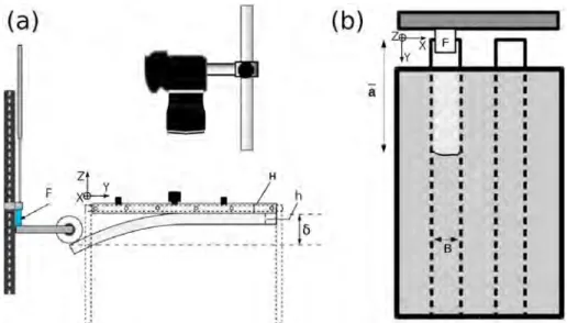
Figure 3. Experimental setup: sketch of (a) side view and (b) top view. F corresponds to the loading force applied to
the narrow plate and𝛿the displacement induced by the normal loading. H designates the large plate height, h the narrow plate height, B the narrow plate width, and̄athe average position of the fracture front with respect to the edge of the narrow plate.
For large earthquakes, typical values for the radiation efficiency,𝜂R, range from 10−2to 1 (Kanamori, 2004). The lowest values of efficiency correspond to slow dynamic rupture events, such as those observed for tsunami earthquakes or some deep earthquakes. Usually the radiation efficiency is obtained for individual seismic event. It then corresponds to a time average representation of the radiated energy from all subfaults comprising the fault plane (Kanamori & Heaton, 2000).
2.4. Influence of the Rupture Velocity
Different theoretical predictions have been proposed for homogeneous interfaces for the dependence of the radiation efficiency on the crack speed, v, according to the fracture modes (Kanamori & Brodsky, 2004). A prediction has been proposed for mode I crack propagation by Freund (1972), Husseini (1977), Kanamori and Brodsky (2004), and Kanamori and Rivera (2006)
𝜂R(v) ∝
v
cr, (9)
where cris the Rayleigh wave speed of the material. Equation (9) predicts that as the rupture speed decreases, the radiation efficiency tends to zero (quasi-static crack propagation). In natural conditions, it has been observed that this radiation efficiency depends on the rupture velocity (Kanamori & Rivera, 2006; Kanamori & Brodsky, 2004). For different types of earthquake, such as deep, intraplate, interplate, or tsunami earth-quakes, it has been shown that one can observe systematically an increase in radiation efficiency as the rupture velocity increases (Venkataraman & Kanamori, 2004). However, the dispersion from the global trend can be important suggesting that other factors can affect the value of𝜂R. It has to be noticed that the theory leading to equation (9) was derived for homogeneous interfaces. Rupture interfaces within the Earth are generally not smooth and host stress heterogeneities (Candela et al., 2011). For example, the energy radi-ated by a quasi-static propagating crack is not zero although its rupture velocity is, on average, very low (i.e., much lower than the Rayleigh wave speed of the material; Heap et al., 2009). Velocity variations of the rupture front are generally observed when detailed imaging of the rupture is obtained (typically in analog experiments; e.g., Måløy et al., 2006). These fluctuations of the rupture velocity are explained by the local pinning and depinning on asperities even if the macroscopic average rupture front velocity is low (Måløy & Schmittbuhl, 2001; Måløy et al., 2006; Stormo et al., 2016). During such slow subcritical ruptures, the exper-imentally recorded acoustic emissions confirm that, locally, dynamic ruptures are occurring (Lengliné et al., 2012; Schmittbuhl et al., 2003).
3. Experimental Setup
Our analog modeling is based on an experimental setup employed for previous studies (Grob et al., 2009; Lengliné, Schmittbuhl, et al., 2011; Måløy et al., 2006; see Figure 3). Samples are made of two transparent
Table 1
Parameters of the Different Experiments
Vload Acoustic Acquisition Average front Sample Experiment (mm/s)a Δ̄a(cm)b devicesc frequency (kHz) velocity (mm/s) configuration
1 0.14 1.2 Z1,Z2,Z3 500 0.92 1 X0Y0Z0 2 0.23 2.1 Z1,Z2,Z3 500 3.7 1 X0Y0Z0 3 0.23 0.61 Z1,Z2,Z3 500 0.60 1 X0Y0Z0 4 0.46 4.2 Z1,Z2,Z3 500 8.1 1 X0Y0Z0 5 0.12 0.51 Z1,Z2,Z3 500 1.1 2 X0Y0Z0 6 0.058 0.43 Z1,Z2,Z3 500 0.34 2 X0Y0Z0 7 0.23 1.4 Z1,Z2,Z3 500 1.3 2 X0Y0Z0 8 0.46 1.3 Z1,Z2,Z3 500 1.7 2 X0Y0Z0 9 0.058 0.22 Z1,Z2,Z3 500 0.19 2 X0Y0Z0 10 0.058 0.69 Z1,Z2,Z3 500 0.48 2 X0Y0Z0 11 0.46 1.3 Y0Z0 2500 3.0 2 12 0.46 1.4 Y0Z0 2500 2.6 2 13 0.46 2.7 Z1,Z2,Z3 500 1.9 2 X0Z0 14 0.058 0.11 Z2 500 0.065 2 15 0.058 0.07 Z2 500 0.044 2 16 0.12 0.23 Z2 500 0.13 2 17 0.46 1.9 Z1,Z2,Z3 500 2.3 2 X0Z0 aV
load: loading velocity in millimeters per second.bΔ̄a = ̄a(tend) −̄a(tstart): average front position displacement during
the experiment, in centimeters. cAcoustic device used during each experiment.
PMMA plates of dimension: 21 × 10.8 × 0.9 cm and 23.1 × 2.5×0.5 cm. The narrower plate is sand blasted on one face with glass beads of diameter𝜑 ∈ [180; 300] 𝜇m. We cleaned blasted plate such as no particles remain on the surface. We then assembled the two plates, the blasted area of the narrower facing the larger plate. We impose on the two plates a normal stress and place the assembly in an oven at 190◦C for 45 min in order to weld the plates together. This procedure creates a weak cohesive interface in an optically transpar-ent material with local random toughness heterogeneities. Introduced asperities induce a spatial toughness distribution with a mean of the order of 150 J/m2and 50% relative fluctuations (Lengliné, Schmittbuhl, et al., 2011). The interface still has an average toughness lower than the bulk of the material (1–2 kJ/m2) pre-scribing the crack front to remain in the weak plane. Once the sample is made, we fix the wider plate to an aluminum structure. A motor applies a displacement at the extremity of the narrow plate in a direction
znormal to the interface. During the loading, we measure the imposed displacement (Linear Variable Dif-ferential Transformer (LVDT)) and the applied force. The displacement imposed by the motor induces a fracture propagation in mode I along y direction (Figure 3). The direction x is set perpendicular to the y and defines the coordinates of a point along the front. Each experiment lasts from 6 to 20 s, depending on the used acquisition frequency (see Table 1). Fracture fronts propagate over few millimeters to centimeters, and
Figure 4. Computation of the crack front position for experiment 1: (a) position of the crack front in red superimposed
over a picture of the crack. The crack propagates from top to bottom. For each picture the crack front is determined as the transition zone between bright and dark areas. (b) Superimposition of the crack positions during the experiment: each line corresponds to a crack position extracted every 0.3 s.
loading velocity is in the range [3 · 10−5to 7 · 10−3]m/s. Details on each experiment parameters are given in Table 1. We implemented two different configurations using the same wide plate but two different narrow plates. Sample configuration 1 corresponds to experiments 1 to 4 and sample configuration 2 to experiments 5 to 17.
3.1. Optical Monitoring
We monitor the crack advance with a camera Nikon D800. The images have a dimension of 1920 × 1080 pixels and a sample resolution of ∼ 52.5 𝜇m/pixel. We recorded optical images at a rate of 30 frames per second. At each time step, we extract the front position in order to monitor the crack front propagation. Extraction of front position is achieved by an image processing algorithm consisting of binarizing the crack front pictures such that we can differentiate the broken and unbroken parts of the sample (Grob et al., 2009). This differentiation is possible due to the sand-blasting procedure introducing heterogeneities at the small plate interface. After annealing the two plates, the sample recovers its transparency. However, on the newly open surface the microstructures along the interface scatter the light and make the area brighter. After converting images in gray scale, (1) we compute differences between each image and the initial one. This step enables the removal of any recurrent background features; (2) gray figures are converted in black and white using a gray level threshold; (3) we compute transition from white to black for each line along the y direction; (4) we extract a(x) as the continuous feature making this transition between the two areas of the
Figure 5. In gray is represented the velocity recorded by one-component
accelerometer Z1during experiment 1. The black line corresponds to the spatial average of the fracture front velocity,⟨V⟩i, along the fracture front at each time step i.
pictures. a(x) then corresponds to the location of the front in the fracture propagation direction y at each time step. By repeating this process at each time frame, we are able to obtain the progression of the crack front, a(x, t), during an experiment (see Figure 4).
We define the average front position in space as̄a(t) = (1∕N)∑Ni=1a(xi, t). The optical acquisition system is triggered by an external TTL signal (+5V) in order to synchronize the optical acquisition with the recording of the acoustic signal.
Fluctuations of average velocity in time are estimated, from frame to frame, during each experiment as V (t) = (̄a(t + 𝛿t) − ̄a(t))∕𝛿t, with
𝛿t = 1∕30 s. Results of this computation are represented in Figure 5.
In order to determine the average front velocity over an experiment, we consider the time window during which velocity is larger than a thresh-old fixed equal to 1 · 10−5m/s. We then compute front velocities⟨V⟩
ion successive intervals i of 1 s. Finally, average front speed⟨V⟩ is estimated over each experiment as the mean value of⟨V⟩i. Fluctuations on velocity values are then estimated as the standard deviation extracted from⟨V⟩i.
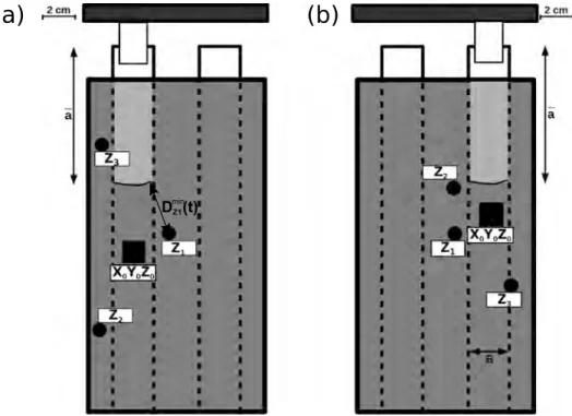
Figure 6. Top views of the two used experimental sample configurations with accelerometer positions on scale.
(a) Experiments 1 to 4. (b) Experiments 5 to 17. Z1,Z2, and Z3are the three one-component accelerometers, and
X0,Y0, and Z0the three-component accelerometer used during each experiment.DminZ1 (t)corresponds to the minimum
distance, at a given time t, between front position and accelerometer Z1. 3.2. Acoustic Monitoring
Acoustic acquisition has been achieved with up to four sensors. We used three one-component accelerom-eters (DeltaTronⓇ, Brüel & Kjær). Their component is vertical and normal to the fracture interface, and we labeled them Z1, Z2, and Z3(cf. Figure 6). We used also an additional three-component accelerometer
(Tri-axial DeltaTronⓇ, Brüel & Kjær; X0, Y0, and Z0, in Figure 6): one component is a normal component, Z0, and the two other components are oriented in the same directions as the axes x and y of the sample. The three vertical accelerometers are placed around the fracture front, and the three-component accelerometer lies directly above the surface of crack propagation (Figure 6). The coupling between each accelerometer and the PMMA plate is ensured using a solid coupling made of phenyl-salicylate. The six accelerometer signals were recorded using two PCI-6133 (National Instruments) acquisition cards (three channels per device). We also recorded the Z0component with a PCI-4744 acquisition device which offers a wider dynamic range of 24 bits compared to 14 bits for the PCI-6133 but limits the sampling frequency to a maximum of 100 kHz (instead of 2.5 MHz for the PCI-6133). The recovered signal in each case is very similar when resampled at the same frequency. This suggests that no distortion is introduced by the recording system and that the res-olution of the PCI-6133 card is sufficient to analyze the recorded waveforms. For most of the experiments, the sampling rate was fixed to 500 kHz. This rate was modified in some experiments to detect a possible influence of the acquisition frequency on our results (see Table 1).
For each acoustic sensor i, and at each time step, we computed two distances Di
min(t)and D i
max(t)which correspond, respectively, to the minimum and maximum distances between the sensor i and the front (Figure 6).
4. Energy Balance Measurements
4.1. Radiated Energy Measurement
4.1.1. Correction for Instrumental Response
Because the recorded waveforms depend on the sensibility of the accelerometer, in order to exploit these sig-nals, we must correct the acquired data from the instrumental response. We call üi(t)the acceleration signal recorded at the sensor i at time t. Instrumental responses, Yi(𝜔), related to each accelerometer, i, have been
Figure 7. (a) Spectrogram of data presented recorded during an experiment by sensor Z1. (b) The corresponding raw
recorded trace by the same accelerometer. Recorded acoustic signal is made of a sum of discrete events with various amplitudes. We note that most of the energy is captured under 100 kHz. Only the largest events produce excitation that are above the noise level at higher frequency.
estimated as a function of the frequency,𝜔. We used various excitation sources to compute the accelerometer response over a wide range of frequency, from 2 Hz to 1.25 MHz. It gives us access to four transfer func-tions: three corresponding to the X0, Y0, and Z0components of the three-component accelerometer and one associated with the one-component accelerometers (see Appendix A). We then convert the raw acceleration recorded at sensor i into a corrected acceleration by taking into account the frequency-dependent sensitivity of the receiver by ̃üi c(𝜔) = ̃üi (𝜔) Yi(𝜔), (10)
where ̃Xdenotes the Fourier transform of variable X and the frequency vector𝜔 ∈ [0; 𝜔Ny], with𝜔Nythe Nyquist frequency; üi
ccorresponds to the acceleration corrected from instrumental responses.
4.1.2. Correction for Attenuation
In order to obtain the radiated energy, we correct the obtained waveform from anelastic attenuation. We have determined attenuation coefficients for the PMMA used in our experiments (see Appendix B). The attenuation law was obtained by comparing the relative amplitude of the acoustic wave recorded at various distances from a common source, sending pulses at various frequencies. We obtained a frequency-dependent attenuation correction that is very comparable to previously reported estimates for this material (Hesham, 2003). The corrected signal, üC, is then calculated as
̃üi C(𝜔) = ̃ü i c(𝜔) · exp ( a ·𝜔 + b 20 ·D i ) , (11)
where Diis the distance from receiver i to front position, a and b are constants determined in Appendix B, and the factor 1/20 appears after the use of decibels to compute attenuation (see Appendix B). We then integrate
Table 2
Results of Computed Energies and Radiation Efficiency
Experiment Gc(J/m2)a E
G(mJ)b ⟨EtotR(tend)⟩(𝜇J)c ⟨𝜂R⟩d
1 82 23.5 1.5 6.3 · 10−5 2 79 40.8 1.1 · 101 2.7 · 10−4 3 82 12.5 7.7 6.2 · 10−4 4 91 93.9 3.3 · 102 3.5 · 10−3 5 171 21.7 1.7 7.9 · 10−5 6 172 18.5 2.4 1.3 · 10−4 7 212 72.6 1.1 · 101 1.5 · 10−4 8 260 81.1 1.2 · 101 1.5 · 10−4 9 247 13.6 3.4 2.5 · 10−4 10 244 42.0 1.1 2.7 · 10−5 11 181 57.6 1.1 · 101 1.8 · 10−4 12 162 56.7 6.1 · 101 1.1 · 10−3 13 95 65.1 2.8 4.3 · 10−5 14 86 2.9 1.1 · 10−3 4.9 · 10−7 15 88 1.4 4.8 · 10−3 3.3 · 10−6 16 95 5.4 1.4 · 10−2 2.7 · 10−6 17 86 40.4 6.9 9.8 · 10−5
aComputed critical energy release rate, G
c, in Joules per meter squared.bFracture
energy, EG, in joule. cAverage radiated energy⟨EtotR (tend)⟩, in joule. dRadiation efficiency,𝜂R.
the resulting signal in order to retrieve a corrected signal in velocity units. This is achieved by computing
̃̇ui C(𝜔) =
̃üi C(𝜔)
2𝜋𝜔 . (12)
As the processing described above introduces noise at low frequency, we applied a high-pass filter (cutoff frequencies𝜔c = 7kHz) to the signal in order to obtain a signal-to-noise ratio as high as possible. We finally transformed the signal back to the time domain by achieving an inverse Fourier transform (Figure 7).
4.1.3. Frequency Content of Acoustic Signal and Asperity Interactions
We checked that the sampling frequency was large enough such that we are not underestimating the radi-ated energy ERby missing some energy at high frequency (Ide & Beroza, 2001). In order to test this, for experiments 11 and 12, we increased the sampling frequency up to 2.5 MHz. Increasing the sampling fre-quency meant that only one sensor was available for recording the experiment. We select this sensor as the closest one to the fracture front such that attenuation effects are as low as possible. This enables us to record any possible high frequencies present in the signal. We find that estimations of radiated energy determined by considering this extended frequency or by resampling the signal at 500 kHz give similar results. We then can assume that a sampling frequency of 500 kHz is high enough for computation of seismic energy emitted by the fracture propagation. This also confirms by our test involving the PICO sensor which is more respon-sive at higher frequency (see Figure S1 in the supporting information). We could see that the acoustic signal emitted by large events and captured both by accelerometers and the PICO sensor has most of its energy below 500 kHz (supporting information).
4.1.4. Combining Multicomponent Measurements
The energy calculated using equation (4) includes the corrected velocity defined in equation (12). It gives us the radiated energy emitted by the whole propagating crack but estimated from a single recording point. Our model does not enable the representation of radiation diagrams associated with each event. However, radiated energy estimates performed at various locations should all yield the same result but depending on the location of sensor with respect to the source radiation diagram; these values slightly differ (see Table S1). The radiated energy is computed dividing the continuous waveform in time windows of 20 ms and treating each time window independently using the actual crack front position that is assigned to this time window.
isotropic and that most of the displacement actually occurs on the horizontal direction. We estimate the ratio𝜖 = EZ0 R∕(E X0 R +E Y0 R +E Z0
R), which indicates the proportion of the radiated energy that is recorded on the vertical component. We found that on average this ratio gives𝜖 = 1∕6.8 (instead of 1/3 for the isotropic case). We consider that this ratio is the same at the location of the other accelerometers (one component), such that we obtain at these locations an estimate of the total radiated energy by dividing the computed energy by the factor𝜖. For the three-component accelerometer, the radiated energy is simply given by the sum of the energy over the three components. Our final estimate of the total seismic energy released during one experiment is obtained as the average over the different sensors after this correction. In some experiments with very slow front propagation, only low-amplitude events were generated such that they can only be recorded by the closest sensor. During experiments 14, 15, and 16, the acoustic signal is solely exploitable from sensor Z2which is the closest to the crack front. In this case, the estimate of the radiated energy is simply computed from the value given by this sensor after applying the coefficient𝜖.
4.2. Fracture Energy Measurement
In order to estimate the fracture energy dissipated during the crack propagation, we follow equation (6) to compute the energy release rate of the system during quasi-static crack propagation at the macroscopic scale. We thus identify Gcas the value G reached by the system when the crack is propagating at a constant speed. Indeed, the crack propagation is a subcritical process: the crack can progress even at a value of G lower than
Gc. We then estimate the critical energy release rate from the plateau value of G during the time the crack is propagating (Lengliné, Schmittbuhl, et al.,2011; Lengliné, Toussaint, & Schmittbuhl et al.,2011). The energy release rate given in equation (7) is computed as
G = −1 B (dU L d̄a ) 𝛿, (13) where B is the narrow plate width, ̄a is the average front position, and 𝛿 implies imposed displacement induced by the applied loading. Noting F the vertical force applied to the narrow plate, the strain energy,
UL, can be expressed as
UL=
F𝛿
2 . (14)
We then obtain, from the beam theory (Lawn & Wilshaw, 1993; Lengliné, Toussaint, et al., 2011) and due to the geometry of our system, that
F =EBH3𝛿
4̄a3 , (15)
where E is the Young modulus of the medium and H its thickness. This yields
UL=
EBH3𝛿2
8̄a3 . (16)
Therefore, we can deduce the following expression of the energy release rate:
G = 3F
2
𝛿
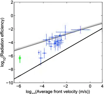
Figure 8. Radiation efficiency𝜂Ras a function of the average fracture front
velocity. Blue diamonds represent averaged results over an experiment and over all available acoustic devices. For these experiments, vertical error bars are related to the use of different accelerometers, while horizontal error bars are associated with front velocity fluctuations over experiments. Green diamond represents results obtained by Goodfellow et al. (2015). The gray lines represent the model defined from equation (21) (from dark to light: mode I, mode II, and mode III; see Appendix D), and the black line is given by equation (9).
Force, displacement, and front position being monitored during each experiment, we can compute the energy release rate using equation (17). Knowing the broken surface during each experiment, we are finally able to obtain EGfrom equation (7) with A = B · (̄a(tend) −̄a(t0))(see Table 2). We observe variations of Gc from an experiment to another (depending on the crack position along the plate) and from a plate to another. These fluctuations of Gcare mostly the result of the sandblast-ing procedure that produces a nonhomogeneous interface and that can display important fluctuations of toughness, with typical standard devi-ation of the order of 50 J/m2as reported in Lengliné, Schmittbuhl, et al. (2011). Obtained values are of the same order of magnitude (∼102J/m2) as previously computed on the same material (Lengliné, Schmittbuhl, et al., 2011).
4.3. Radiation Efficiency
The estimates of EGand ERfor each experiment are used to compute the radiation efficiency,𝜂R, as defined by equation (8). For each experiment, the value of ERcorresponds to the average estimate over all available sen-sors. We find that the ratio𝜂Rranges between 4.9 · 10−7and 3.5 · 10−3 (Table 2).
As shown in Figure 8, the radiation efficiency shows a positive depen-dence with the average rupture velocity. The observed slope in the log-log diagram indicates a power law relation between the average fracture speed and the seismic radiation efficiency: the higher the velocity, the higher the efficiency. Fracture front velocity is determined using the opti-cal monitoring of each experiment. Velocities represented in Figure 8 are computed using the average propagation speed during the crack advance. During one of the experiments, the assumption of quasi-static rupture propagation was not verified and the front jumped rapidly to a new equilibrium position. We decided to isolate this fast rupture event from exper-iment 4 and to treat it as a separate experexper-iment of short duration (200 ms). Although we captured only one image of this fast event, the acoustic signal shows that multiple acoustic events were generated. We also present in Figure S2 the same results as in Figure 8, but instead of considering average quantities for each experiment, we decomposed each of them in time intervals of 0.8 s.
5. Modeling the Relationship Between Radiation Efficiency and Rupture
Velocity
We compare our experimental results with two different approaches relating fracture front velocity to radiation efficiency.
5.1. Homogeneous Velocity
On the one hand, our results are compared with the theoretical model introduced in equation (9) and pro-posed for mode I cracks (Husseini, 1977; Kanamori & Brodsky, 2004; Kanamori & Rivera, 2006). It relates radiation efficiency and crack velocity, v, for a mode I propagating fracture along a homogeneous interface. Equation (9) shows that the prediction always underestimates our observations of𝜂Rfor the whole range of rupture speed resolved in our experiments. Such an observation is not totally surprising as equation (9) was obtained considering a homogeneous interface.
5.2. Heterogeneous Velocity
The introduction of asperities in our model is responsible for the deviation of our results from equation (9). Locally, although the average crack propagation is slow and uniform (stable subcritical regime), dynamic ruptures are occurring involving local fracture velocity variations (Schmittbuhl et al., 2003). It has been shown that, in this case, the local crack front velocity can be well described by a power law decay function above the average crack front velocity⟨v⟩. Indeed, (Måløy et al., 2006) have shown that, when discretized in
Figure 9. (a) Estimate of the influence of the average fracture velocity⟨v⟩on the radiation efficiency𝜂Rfor different values of𝛾∗from our statistical model. (b) Evolution of the𝛼exponent:𝜂
R ∝ ⟨v⟩𝛼as a function of𝛾∗. time, the rupture velocity v follows
𝑓(v) ∝ ( v ⟨v⟩ )−𝛾 , (18)
with f(v) the velocity distribution function for v > ⟨v⟩. Such a relation has been tested over a wide range of ⟨v⟩ although considering only slow crack front displacements (v ≪ cr). The power law exponent𝛾 found for all tested experiments is always close to a universal value for a random distribution of asperities:𝛾 = 2.55 (Måløy et al., 2006) and is well supported by direct numerical modeling (Stormo et al., 2016). If we consider the distribution of velocity but discretized over space, the shape of the distribution is preserved but the power law exponent is𝛾∗ = 𝛾 − 1 (see Appendix C). We introduced an exponential cutoff at low velocity to model the complete distribution of the local crack velocity over the whole velocity range (Lengliné et al., 2012; Måløy et al., 2006). Then, the probability distribution of the rupture velocity for a front propagating at an average speed⟨v⟩ can be expressed as
𝑓∗(v) = K ( v ⟨v⟩ )−𝛾∗ exp ( −⟨v⟩ v ) , (19)
where K is an integration constant defined such that 1 = ∫
cr 0
The probability density function defined in equation (19) has been shown to represent a correct description of the local velocity distribution at various spatial scales (Anderson, 2005; Jestin et al., 2018). It implies that there is no spatial scale associated with this distribution down to the smallest resolvable scale and up to the largest scale, arguing that the same mechanical process is responsible for the crack advance at these different scales. Moreover, the process zone size has been estimated to be of the order of 10𝜇m. As the probability density function of the local front velocity is scale invariant, we can conclude that the use of equation (19) is correct in the LEFM approach.
Then, the radiation efficiency for a model of heterogeneous rupture speed is given by the product of the probability of each velocity, f(v), and of the actual radiation efficiency of the given rupture speed interval assuming equation (9) to be valid for this velocity range that is
𝜂∗ R(⟨v⟩) = ∫ cr 0 K ( v ⟨v⟩ )−𝛾∗ exp ( −⟨v⟩ v ) ( v cr ) dv, (21) where𝜂∗
R(⟨v⟩) represents the computed radiation efficiency for heterogeneous interface at the average rup-ture speed⟨v⟩. We note that, using equation (21), we hypothesize that the rupture speed distribution in our experiments is distributed following the power law function given by equation (19) up to the Rayleigh wave speed, cr. So far, in all conducted experiments, we always observe the trend predicted by equation (19) up to the highest possible fracture speed allowed by an optical monitoring system (Måløy et al., 2006). Yet even at this highest speed we still are far from cr. We nonetheless compare these estimates of𝜂∗Rwith our results. We notice, in Figure 8, that these modeled predictions seem to better estimate our radiation efficiencies determined in our experiments than the model described by equation (9).
We can see from Figure 8 that we can well approximate equation (21) by a power law such as𝜂R ∝ ⟨v⟩𝛼. We then obtained a relationship between the exponents𝛼 and 𝛾∗. Figure 9 shows the impact of a variation in𝛾∗ values (i.e., in fracture velocity distribution) on the slope of the gray curve in Figure 8. As𝛾∗increases, that is, the local speed values get close to the average value⟨v⟩, the exponent 𝛼 converges to 1 and we get close to the model associated with a homogeneous interface. On the contrary, if𝛾∗decreases, the speed distribution expands (i.e., the local velocities vary over a wide range of values),𝛼 decreases and the average fracture velocity is no longer significant enough to describe the global rupture occurring in our medium. Our value of𝛾∗, established by Måløy et al. (2006), seems to well describe the impact of the asperities on the fracture surface on our results of𝜂R.
6. Discussion
6.1. Comparison With Other Experimental Measurements
Some previous investigations of the radiated energy from propagating cracks were performed experimen-tally. We notably compare our results to values reported in a similar experimental setup geometry and loading. Radiation efficiency was measured in these experiments for mode I crack in PMMA and soda-lime glass (Boler, 1990; Boler & Spetzler, 1986; Gross et al., 1993). In all of these studies, the crack velocity was much higher than in our experiment (from 35 to 2,000 m/s). Radiation efficiency computed from the results reported in Boler and Spetzler (1986) ranges between 10−5and 10−3. The experiments performed in Gross et al. (1993) show that the radiation efficiency is closer to 10−2. We can also compare our observations to results obtained with hydraulic fracture experiments in rocks (Goodfellow et al., 2015). In this study, radi-ation efficiency, close to the ratio between the radiated energy and the change in elastic energy, has been estimated, for opening crack in Westerly granite, ranging from 10−7to 10−6. Because of the used experimen-tal setup, the macroscopic crack velocity cannot be measured precisely. However, if we consider the axial displacement observed during the whole experiment, we can estimate an average crack velocity close to 1
𝜇m/s. These results seem to be in agreement with equations (9) and (21).
6.2. On the Role of Asperities in the Fracture Processes 6.2.1. Effect of Asperities in Radiation Efficiency
Our results show that the heterogeneous nature of the rupture velocity field over the interface can lead to sig-nificant deviation of the radiated energy compared to the predicted value from a homogeneous approach. In our modeling of equation (21) we have made the hypothesis that the velocity distribution over the whole fault surface can be described by a continuous power law function for velocities higher than the average speed. It is readily possible that such a parametrization of the velocity represents an oversimplification. Indeed, the power law exponent describing the rupture speed probability density function may vary when approaching
(Gudmundsson et al., 2002). In these contexts, the fracture speed appears to be controlled by the fluid injec-tion. Our results then suggest that adjusting the flow rate is expected to be a tool to reduce the radiation efficiency and to develop more aseismic slip and less induced seismicity for a given pressure. Furthermore, mode I fractures are also very commonly studied in rock laboratory experiments in order to investigate the rock failure mechanism (Atkinson, 1984). In many instances, a seismic signal related to the propagation of the mode I fracture can be recorded. While in some cases this signal does not reflect the failure condition at the crack tip but is related to shear-induced events on weak interfaces in the fracture vicinity (Rubin & Gillard, 1998); there are some evidences of recorded signal representing tensile rupture events (Fischer & Guest, 2011; Majer & Doe, 1986; Šílen `y et al., 2009). In this context it is possible to estimate the radiated energy of the fracture from the recorded seismic signal. When locations are available, it is also possible to compute the rupture velocity of the propagating fracture from the migration of the seismic events. With these two quantities and using equation (21) one can therefore obtain the strength of the formation provid-ing an estimate of the heterogeneity of the fractured media,𝛾, or inversely characterize this last quantity if one instead have an estimate of Gc, for example, through laboratory testing. Our results can also be imple-mented in such a way that one can predict the radiated energy caused by a slowly propagating fracture. Assuming a linear relationship between the seismicity rate (i.e., the number of events per unit of time) and the average velocity (R ∝ v) as demonstrated in Lengliné et al. (2012), one would predict that the seismic-ity rate will evolve as R ∝ 𝜂(1∕0R .55)which is close to a quadratic behavior. This can have implications, for example, when one tries to estimate the seismic activity of stimulated geothermal reservoirs.
A natural step is to extend our results to the shear crack modes (mode II and mode III). We acknowledge that, in natural conditions, most of the ruptures within the Earth stress field are best represented by shear ruptures (mode II and mode III). The equation that governs the stress field at the tip of the crack and consequently the advance of the crack front is very similar for all three modes of rupture (Gao et al., 1991). Indeed, the local fluctuations of the stress field at the tip of the propagating crack depends on the existing elastic interactions. The elastic kernel that describes these interactions is very similar for all rupture modes and only differs by a prefactor. It then led to models of shear crack that have strong similarities with mode I crack (Gao et al., 1991; Jestin et al., 2018).
Fundamentally, as shown from our experimental results, the integrated radiation efficiency will depend on the velocity distribution f(v) and on g(v) as stated by equation (21). Transposing these results in terms of shear failure would imply using the appropriate form of g(v) (see Appendix D) and using a description of f(v) for mode II or mode III ruptures. We can see that if the corresponding mode II and mode III dependence of the radiation efficiency on rupture velocity is applied on our actual velocity distribution, the difference of the predicted radiation efficiency between the different rupture modes is negligible compared to the difference with the experimental results. (see Figure 8 and ArefapD). Unfortunately, there is no such distribution of f(v) for natural shear ruptures, mostly because it requires instruments capable of monitoring fault movements with a high resolution and sampling frequency. While the quantitative analysis for mode II/mode III crack will require the detail knowledge of the rupture velocity distribution, we still point that the presence of asperities will control the shape of this distribution such that the results obtained in our mode I setup with a heterogeneous interface are conceptually similarly valid on a more general aspect of heterogeneous slow rupture, in particular if slip is small compared to the asperity size. It therefore points on the role of the shear fracture interface properties on modulating the radiated energy of a propagating crack. Notably, it implies that for a same rupture speed, a crack will tend to radiate more energy if its propagation is less homogeneous.
Conclusion
This study describes the energy partitioning for slow deformation during the mode I propagation of fracture along a heterogeneous interface. We evaluated the radiation efficiency that characterizes the proportion of the energy radiated in form of seismic waves. We explored the dependence of the radiation efficiency on the macroscopic crack front velocity in the subcritical propagation domain. We noticed, a nonlinear increase of the radiation efficiency with the average fracture front propagation velocity:𝜂R ∝ ⟨v⟩0.55. This trend is in agreement with a simple model based on the power law distribution of the local rupture velocities. The presence of asperities on the fault surface is shown to generate differences with previously presented models that only considered propagation over a homogeneous interface.
Data and Resources
All data obtained in our experiments are available at https://dx.doi.org/10.25577/2019-Jestin-JGR.
Appendix A: Transfer Functions Computation
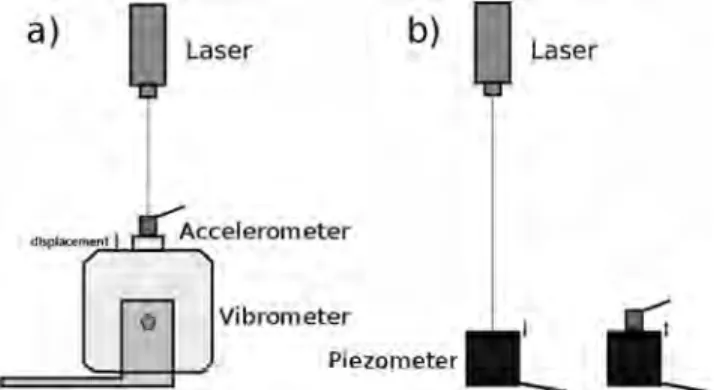
Calibration of accelerometers has been achieved by recording the response from a common excitation source by both the accelerometers and a laser vibrometer. The laser is a CLV-2534, a Compact Laser Vibrometer produced by Polytec. This device records a velocity, and its signature is known to be flat. In order to easily inspect the devices' responses to a large range of frequencies, a sweep signal is sent to an excitation source. The produced vibrations are then recorded by the laser or the accelerometer. The sweep signal is a sinusoid of a constant amplitude but with a frequency increasing with time. Two kinds of sources have been employed in our calibration setups: a mechanical vibrometer pulsing from 2 Hz to 18 kHz (Figure A1, left) and a piezometer source used in active mode and sending signals from 1 kHz to 1.25 MHz (Figure A1, right). All signals were digitized by two different acquisition systems. We checked that the acquisition system does not introduce any modification of the recorded signals.
For all possible frequency ranges, we compute the ratio between the Fourier transform of the accelerometer and laser signals. We smooth and average our results to obtain transfer function for a bandwidth going from 2 Hz to 1.25 MHz. Figure A2 shows results obtained for one-component accelerometers. This procedure enables us to assess an accurate instrumental correction.
Appendix B: PMMA Attenuation
In order to determine the anelastic attenuation in the PMMA plate in our experiments, we send a signal using a source piezometer attached to the PMMA sample. The signal is a sine pulse, which frequency varies for different tests. Receiver is placed on the other side of the plate, facing the source (see Figure B1). Records start at the time the pulse is emitted from the source. The sampling frequency is fixed at 2.5 MHz. For each experiment, we stacked 100 records in order to improve the signal-to-noise ratio.
We suppose that the reflection of the acoustic waves on the PMMA surface is total. Then, the decrease of the signal amplitude with time enables the computation of the attenuation coefficient (Figure B2). We
Figure A1. Calibration setups. (a) The configuration involving the vibrometer. In this case, records of source signal are
simultaneously achieved by accelerometer and laser. (b) The employed source is a piezometer. In this setup, laser and accelerometer records are done one after the other but triggered so that measures begin at the same frequency.
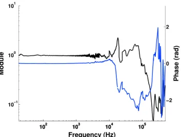
Figure A2. Calibration results for one-component accelerometers. The black line corresponds to the transfer function
module, and the blue line represents its phase.
compute the envelope of the recorded signal, and we extract from the envelope the ratio between maximum amplitude, Amax, and the amplitude at each distance, Ai. We computed the trave-led distance as function of time, considering the velocity of the P wave equal to 2,700 m/s. We get the slope𝜅 relating Y = 20 · log( Ai
Amax ) to the distance step xi.𝜅 is called the attenuation factor and is expressed in terms of decibels per meter. Experiments are done on two plate widths: a 9.8-mm plate and a 3-cm plate. The use of these two differ-ent plate widths gives similar values. Results are presdiffer-ented in Figure B3. We find the relation between the attenuation coefficient𝜅 and the source frequency fsourceto be
𝜅 = a · 𝑓source−b, (B1)
with a = 1.4 · 10−4and b = 56.
Appendix C: Velocity Probability Distribution Function: From Spatiotemporal
to Spatial Domain
Following the derivation presented in Tallakstad et al. (2011), we make the transformation from spatiotem-poral to spatial expression of the map of local velocity related to the considered fracture. Let us consider
Vt(x, t), the spatiotemporal map of velocity associated to the probability distribution function, P(v) and
V(x, y), the spatial map associated with the function Q(v). We can write dy = vdt. The area in space where
the front travels at speed u between v and v + dv corresponds to the total area of fracture propagation Ax,y multiplied by the fraction of area corresponding to this velocity
∫v<u(x,𝑦)<v+dvdxd𝑦 = Ax,𝑦R(v)dv. (C1)
Figure B1. Experimental setup: the source (piezometer) is placed directly in front of the receiver (accelerometer). The
Figure B2. Example of a recorded signal for a source frequency of 250 kHz. In blue are represented the absolute values
of the records and in red the envelope of this signal used for the attenuation estimations.
If we apply a change of variable from y to t, we can write
∫v<u(x,𝑦)<v+dvdxd𝑦 = ∫v<u(x,t)<v+dvdxvdt. (C2) Denoting Ax,tthe total area of the spatio-temporal map, we have
∫v<u(x,t)<v+dvdxdt = Ax,tP(v)dv. (C3)
Moreover, we have Ax,y∕Ax,t = ⟨v⟩. Thus,
⟨v⟩R(v)dv = P(v)vdv, (C4) which leads to R(v) = A · ( v ⟨v⟩ )−𝛾+1 . (C5)
Figure B3. Computed attenuation coefficients as a function of the wave frequency. In red are represented values
obtained with a 3cm-width-PMMA plate and in blue values for the 98mm-width-plate. In black is presented the best data fitting.
1 −𝛽v g(v) = √ √ √ √ √1 − v 𝛽 1 +𝛽v, (D4)
respectively, for mode I cracks, for mode II cracks, and for mode III cracks (Kanamori & Rivera, 2006). In order to better understand the differences between these three relations, we input them in equation (21) and present results associated with the different modes of crack in Figure 8. We then observe a limited impact of the loading mode on the model related to equation (21).
References
Anderson, T. L. (2005). Fracture mechanics: Fundamentals and applications (3rd ed.). Boca Raton: CRC Press.
Atkinson, B. K. (1984). Subcritical crack growth in geological materials. Journal of Geophysical Research, 89(B6), 4077–4114. Atkinson, B. K. (1987). Fracture mechanics of rock, Academic Press Geology Series. London: Elsevier.
Ben-Zion, Y. (2008). Collective behavior of earthquakes and faults: Continuum-discrete transitions, progressive evolutionary changes, and different dynamic regimes. Reviews of Geophysics, 46, RG4006. https://doi.org/10.1029/2008RG000260
Ben-Zion, Y., & Sammis, C. G. (2003). Characterization of fault zones. Pure and Applied Geophysics, 160, 677–715.
Boler, F. M. (1990). Measurements of radiated elastic wave energy from dynamic tensile cracks. Journal of Geophysical Research, 95(B3), 2593–2607.
Boler, F. M., & Spetzler, H. (1986). Radiated seismic energy and strain energy release in laboratory dynamic tensile fracture. Pure and
Applied Geophysics, 124, 759–772.
Brossman, M. W., & Kies, J. A. (1955). Energy release rates during fracturing of perforated plates. NRL Memorandum Report, 370, 1–21. Brudy, M., & Zoback, M. (1999). Drilling-induced tensile wall-fractures: Implications for determination of in-situ stress orientation and
magnitude. International Journal of Rock Mechanics and Mining Sciences, 36(2), 191–215.
Candela, T., Renard, F., Schmittbuhl, J., Bouchon, M., & Brodsky, E. E. (2011). Fault slip distribution and fault roughness. Geophysical
Journal International, 187, 959–968.
Farin, M., Mangeney, A., De Rosny, J., Toussaint, R., Sainte-Marie, J., & Shapiro, N. M. (2016). Experimental validation of theoretical methods to estimate the energy radiated by elastic waves during an impact. Journal of Sound and Vibration, 362, 176–202.
Fialko, Y. (2007). Fracture and frictional mechanics—Theory (pp. 95–98). La Jolla, CA, USA: Elsevier B.V.
Fischer, T., & Guest, A. (2011). Shear and tensile earthquakes caused by fluid injection. Geophysical Research Letters, 38, L05307. https://doi.org/10.1029/2010GL045447
Freund, L. B. (1972). Energy flux into the tip of an extending crack in an elastic solid. Journal of Elasticity, 2, 341–349.
Gao, H., Rice, J. R., & Lee, J. (1991). Penetration of a quasi-statically slipping crack into a seismogenic zone of heterogeneous fracture resistance. Journal of Geophysical Research, 96(B13), 21,535–21,548.
Geertsma, J., & De Klerk, F. (1969). A rapid method of predicting width and extent of hydraulically induced fractures. Society of Petroleum
Engineers, 21(12), 1571–1582.
Goodfellow, S. D., Nasseri, M. H. B., Maxwell, S. C., & Young, R. P. (2015). Hydraulic fracture energy budget: Insights from the laboratory.
Geophysical Research Letters, 42, 3179–3187. https://doi.org/10.1002/2015GL063093
Grob, M., Schmittbuhl, J., Toussaint, R., Rivera, L., Santucci, S., & Måløy, K. J. (2009). Quake catalogs from an optical monitoring of an interfacial crack. Pure and Applied Geophysics, 166, 777–799.
Gross, S. P., Fineberg, J., Marder, M., McCormick, W. D., & Swinney, H. L. (1993). Acoustic emissions from rapidly moving cracks.
Biophysical Reviews and Letters, 71, 3162–3165.
Gudmundsson, A. (2011). Rock fractures in geological processes. Cambridge: Cambridge University Press.
Gudmundsson, A., Fjeldskaar, I., & Brenner, S. L. (2002). Propagation pathways and fluid transport of hydrofractures in jointed and layered rocks in geothermal fields. Journal of Volcanology and Geothermal Research, 116(3), 257–278.
Haskell, N. A. (1964). Total energy and energy spectral density of elastic wave radiation from propagating faults. Bulletin of the Seismological
Society of America, 56, 125–140.
Heap, M. J., Baud, P., Meredith, P. G., Bell, A. F., & Main, I. G. (2009). Time-dependent brittle creep in Darley Dale sandstone. Journal of
Geophysical Research, 114, B07203. https://doi.org/10.1029/2008JB006212
Acknowledgments
We are very grateful to Alain Steyer for his technical support. We thank L. Rivera for his detailed review of this manuscript and H. Karabulut, M. Bouchon, J. P. Ampuero, and Z. Duputel for fruitful discussions. We thank M. Heap for grammatical assistance.
Hesham, A. (2003). Ultrasonic pulse echo studies of the physical properties of PMMA, PS, and PVC. Polymer - Plastics Technology and
Engineering, 42, 193–205.
Husseini, M. I. (1977). Energy balance for motion along a fault. Journal of Geophysical Research, 49, 699–714.
Ide, S., & Beroza, G. C. (2001). Does apparent stress vary with earthquake size? Geophysical Research Letters, 28, 3349–3352. Irwin, G. R., & Kies, J. A. (1954). Critical energy rate analysis of fracture strength. Welding and Joining, 4763, 193–198.
Jestin, C., Lengliné, O., & Schmittbuhl, J. (2018). Mode-III interfacial crack propagation in heterogeneous media. Physical Review E, 97, 63004.
Julian, B. R., Foulger, G. R., Monastero, F. C., & Bjornstad, S. (2010). Imaging hydraulic fractures in a geothermal reservoir. Geophysical
Research Letters, 37, L07305. https://doi.org/10.1029/2009GL040933
Kanamori, H. (2004). The diversity of the physics of earthquakes. Proceedings of the Japan Academy, Ser. B, Physical and Biological Sciences,
80, 297–316.
Kanamori, H., & Brodsky, E. E. (2004). The physics of earthquakes. Reports on Progress in Physics, 67, 1429–1496.
Kanamori, H., & Heaton, T. H. (2000). Microscopic and macroscopic physics of earthquakes. Geophysical Monograph, 120, 147–163. Kanamori, H., & Rivera, L. (2006). Energy partitioning during and earthquake. Geophysical Monograph, 120, 147–163.
Lawn, B., & Wilshaw, T. R. (1993). Fracture of brittle solids (2nd ed.). Cambridge: Cambridge University Press.
Lengliné, O., Elkhoury, J., Daniel, G., Schmittbuhl, J., Toussaint, R., Ampuero, J. P., & Bouchon, M. (2012). Interplay of seismic and aseismic deformations during earthquake swarms: An experimental approach. Earth and Planetary Science Letters, 331-332, 215–223. Lengliné, O., Schmittbuhl, J., Elkhoury, J. E., Ampuero, J. P., Toussaint, R., & Måløy, K. J. (2011). Downscaling of fracture energy during
brittle creep experiments. Journal of Geophysical Research, 116, B08215. https://doi.org/10.1029/2010JB008059
Lengliné, O., Toussaint, R., & Schmittbuhl, J. (2011). Average crack-front velocity during subcritical fracture propagation in a heterogeneous medium. Physical Review E, 84, 36104.
Måløy, K. J., Santucci, S., Schmittbuhl, J., & Toussaint, R. (2006). Local waiting time fluctuations along a randomly pinned crack front.
Physical Review Letters, 96, 45501.
Måløy, K., & Schmittbuhl, J. (2001). Dynamical events during slow crack propagation. Physical Review Letters, 87(10), 105502.
Majer, E. L., & Doe, T. W. (1986). Studying hydrofractures by high frequency seismic monitoring. International Journal of Rock Mechanics
and Mining Sciences & Geomechanics Abstracts, 23(3), 185–199.
Marsan, D. (2006). Can coseismic stress variability suppress seismicity shadows? Insights from a rate-and-state friction model. Journal of
Geophysical Research, 111, B06305. https://doi.org/10.1029/2005JB004060
Maxwell, S. C., Rutledge, J., Jones, R., & Fehler, M. (2010). Petroleum reservoir characterization using downhole microseismic monitoring.
Geophysics, 75(75A), 129–137.
Nasseri, M. H. B., Mohanty, B., & Young, R. P. (2006). Fracture toughness measurements and acoustic emission activity in brittle rocks.
Pure and Applied Geophysics, 163(5-6), 917–945.
Okubo, P. G., & Aki, K. (1987). Fractal geometry in the San Andreas fault system. Journal of Geophysical Research, 92(B1), 345–355. Ripperger, J., Ampuero, J. P., Mai, P. M., & Giardini, D. (2007). Earthquake source characteristics from dynamic rupture with constrained
stochastic fault stress. Journal of Geophysical Research, 112, B04311. https://doi.org/10.1029/2006JB004515
Rubin, A. M. (1993). Tensile fracture of rock at high confining pressure—Implications for dike propagation. Journal of Geophysical Research,
98(B9), 15,919–15,935.
Rubin, A. M., & Gillard, D. (1998). Dike-induced earthquakes: Theoretical considerations. Journal of Geophysical Research, 103(B5), 10,017–10,030.
Schmittbuhl, J., Chambon, G., Hansen, A., & Bouchon, M. (2006). Are stress distributions along faults the signature of asperity squeeze?
Geophysical Research Letters, 33, L13307. https://doi.org/10.1029/2006GL025952
Schmittbuhl, J., Delaplace, A., Måløy, K. J., Perfettini, H., & Vilotte, J. P. (2003). Slow crack propagation and slip correlations. Pure and
Applied Geophysics, 160, 961–976.
Scholz, C. H. (2002). The mechanics of earthquakes and faulting. Cambridge: Cambridge University press.
Stormo, A., Lengliné, O., Schmittbuhl, J., & Hansen, A. (2016). Soft-clamp fiber bundle model and interfacial crack propagation: Comparison using a non-linear imposed displacement. Frontiers of Physics, 4(18), 18–28.
Tallakstad, K. T., Toussaint, R., Santucci, S., Schmittbuhl, J., & Måløy, K. J. (2011). Local dynamics of a randomly pinned crack front during creep and forced propagation: An experimental study. Physical Review E, 83(4), 46108.
Turkaya, S., Toussaint, R., Eriksen, F. K., Lengliné, O., Daniel, G., Flekkøy, E. G., & Måløy, K. J. (2016). Note: Localization based on estimated source energy homogeneity. Review of Scientific Instruments, 87(9), 96101.
Udías, A., Madariaga, R., & Buforn, E. (2014). Source mechanisms of earthquakes: Theory and practice. Cambridge, New York: Cambridge University Press.
Venkataraman, A., & Kanamori, H. (2004). Observational constraints on the fracture energy of subduction zone earthquakes. Journal of
Geophysical Research, 109, B05302. https://doi.org/10.1029/2003JB002549 Yoshiyama, A. (1963). Note on earthquake energy. Bull. Earthquake Res. Inst.
Šílen `y, J., Hill, D. P., Eisner, L., & Cornet, F. H. (2009). Non–double-couple mechanisms of microearthquakes induced by hydraulic fracturing. Journal of Geophysical Research, 114, B08307. https://doi.org/10.1029/2008JB005987