HAL Id: hal-00296293
https://hal.archives-ouvertes.fr/hal-00296293
Submitted on 24 Jul 2007
HAL is a multi-disciplinary open access
archive for the deposit and dissemination of
sci-entific research documents, whether they are
pub-lished or not. The documents may come from
teaching and research institutions in France or
abroad, or from public or private research centers.
L’archive ouverte pluridisciplinaire HAL, est
destinée au dépôt et à la diffusion de documents
scientifiques de niveau recherche, publiés ou non,
émanant des établissements d’enseignement et de
recherche français ou étrangers, des laboratoires
publics ou privés.
ozone and ozone-related species over Poker Flat (65° N,
147° W), Alaska observed by a ground-based FTIR
spectrometer from 2001 to 2003
A. Kagawa, Y. Kasai, N. B. Jones, M. Yamamori, K. Seki, F. Murcray, Y.
Murayama, K. Mizutani, T. Itabe
To cite this version:
A. Kagawa, Y. Kasai, N. B. Jones, M. Yamamori, K. Seki, et al.. Characteristics and error estimation
of stratospheric ozone and ozone-related species over Poker Flat (65° N, 147° W), Alaska observed by a
ground-based FTIR spectrometer from 2001 to 2003. Atmospheric Chemistry and Physics, European
Geosciences Union, 2007, 7 (14), pp.3791-3810. �hal-00296293�
www.atmos-chem-phys.net/7/3791/2007/ © Author(s) 2007. This work is licensed under a Creative Commons License.
Chemistry
and Physics
Characteristics and error estimation of stratospheric ozone and
ozone-related species over Poker Flat (65
◦
N, 147
◦
W), Alaska
observed by a ground-based FTIR spectrometer from 2001 to 2003
A. Kagawa1,2, Y. Kasai2, N. B. Jones3, M. Yamamori2,4, K. Seki2,5, F. Murcray6, Y. Murayama2,7, K. Mizutani2, and T. Itabe2
1Fujitsu FIP Corporation, Tokyo, Japan
2National Institute of Information and Communications Technology, Tokyo, Japan 3Wollongong University, Wollongong, Australia
4Tsuru University, Yamanashi, Japan
5Mitsubishi Electric Corporation, Kanagawa, Japan 6University of Denver, Denver, USA
7National Institute of Polar Research, Tokyo, Japan
Received: 4 August 2006 – Published in Atmos. Chem. Phys. Discuss.: 17 October 2006 Revised: 16 April 2007 – Accepted: 13 July 2007 – Published: 24 July 2007
Abstract. It is important to obtain the year-to-year trend of
stratospheric minor species in the context of global changes. An important example is the trend in global ozone depletion. The purpose of this paper is to report the accuracy and preci-sion of measurements of stratospheric chemical species that are made at our Poker Flat site in Alaska (65◦N, 147◦W). Since 1999, minor atmospheric molecules have been ob-served using a Fourier-Transform solar-absorption infrared Spectrometer (FTS) at Poker Flat. Vertical profiles of the abundances of ozone, HNO3, HCl, and HF for the period from 2001 to 2003 were retrieved from FTS spectra us-ing Rodgers’ formulation of the Optimal Estimation Method (OEM). The accuracy and precision of the retrievals were es-timated by formal error analysis. Errors for the total column were estimated to be 5.3%, 3.4%, 5.9%, and 5.3% for ozone, HNO3, HCl, and HF, respectively. The ozone vertical pro-files were in good agreement with propro-files derived from col-located ozonesonde measurements that were smoothed with averaging kernel functions that had been obtained with the retrieval procedure used in the analysis of spectra from the ground-based FTS (gb-FTS). The O3, HCl, and HF columns that were retrieved from the FTS measurements were con-sistent with Earth Probe/Total Ozone Mapping Spectrometer (TOMS) and HALogen Occultation Experiment (HALOE) data over Alaska within the error limits of all the respective datasets. This is the first report from the Poker Flat FTS ob-Correspondence to: A. Kagawa
servation site on a number of stratospheric gas profiles in-cluding a comprehensive error analysis.
1 Introduction
Stratospheric ozone depletion has been observed at mid-latitudes for the past several decades (WMO, 2003). Hetero-geneous chemical reactions play an important role in middle latitude ozone loss. Organic halogen species such as CFC’s eventually break down into inactive forms in the stratosphere, forming reservoir species (e.g., HCl). Heterogeneous reac-tions at mid-latitudes result in changes to the partitioning of NOy and prevent conversion of active halogen species that destroy ozone into inactive ones.
Because the long-term trend in stratospheric ozone is ex-pected to be linked to loading of chlorine and bromine species in the stratosphere, recent focus of research has been on recovery of the ozone layer, since chlorine loading ap-pears to be near its peak in the stratosphere (Newchurch et al., 2003). Rinsland et al. (2003b) studied the long-term trend of Cly using FTS data from multiple Network Detection of Atmospheric Composition Change (NDACC, http://www.ndsc.ncep.noaa.gov/, formerly NDSC). observa-tion sites, and reported increasing Clyuntil the early 1990s, reaching a plateau at the end of 1990s. Because ozone variability is not only affected by halogen species but also by other factors such as stratospheric temperature changes
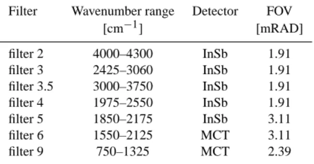
Table 1. Filters, their wavenumber ranges, detectors, and Field-of-views used for the FTS measurements at Poker Flat.
Filter Wavenumber range Detector FOV [cm−1] [mRAD] filter 2 4000–4300 InSb 1.91 filter 3 2425–3060 InSb 1.91 filter 3.5 3000–3750 InSb 1.91 filter 4 1975–2550 InSb 1.91 filter 5 1850–2175 InSb 3.11 filter 6 1550–2125 MCT 3.11 filter 9 750–1325 MCT 2.39
coming from increases in greenhouse gases, a cautious ap-proach must be taken in detecting the recovery of the ozone layer as a response to halogen loading in the stratosphere. The detection of this recovery phase has therefore been in-tensively investigated (Newchurch et al., 2003; Reinsel et al., 2005). Monitoring stratospheric ozone and ozone-related species is still important because of the complicated condi-tions surrounding the stratospheric ozone layer.
There have been many studies on the variability of stratospheric ozone and ozone-related species from satellite, balloon-borne, and ground-based (gb) observations (Fioletov et al., 2002; Manney et al., 1997; Wang et al., 2002). Because ozone and many ozone-related species have absorptions in the infrared region, Fourier transform infrared (FTIR) spec-trometers are highly suited to measurements of atmospheric molecules related to ozone; they can be used to analyze so-lar and lunar absorption spectra as well as emissions from the atmosphere. Many molecules have been monitored us-ing ground-based FTS systems within the framework for the NDACC. In particular, minor species related to stratospheric ozone have been extensively studied using ground-based FTS (Barret et al., 2002, 2003, 2005; Goldman et al., 1999; Hase et al., 2004; Nakajima et al., 1997; Paton-Walsh et al., 1997; Pougatchev et al., 1996; Rinsland et al., 2000; Schneider et al., 2005a, 2005b; Wood et al., 2002, 2004). The merit of us-ing ground-based FTS for atmospheric measurements is that an FTS can simultaneously observe many molecules over a wide range of wavelengths. Modern FTS systems are also optically stable and are therefore suited to long-term obser-vations (∼10 years).
We have been observing solar absorption spectra over Poker Flat (65.1◦N, 147.4◦W, 0.61 km), Alaska since 1999 by using a high-resolution FTS, as a part of the Alaska Project. The Alaska Project is an international collaboration between the National Institute of Information and Communi-cations Technology (NICT) (formerly the CommuniCommuni-cations Research Laboratory (CRL)) and the University of Alaska Fairbanks (UAF) in which many instruments are used to in-vestigate the atmospheric environment from the troposphere to the thermosphere (Murayama et al., 2003).
Poker Flat is located between the Arctic region and mid-latitudes. Because it is outside the polar vortex for most of the winter and spring in the lower and middle stratosphere, the gas phase and heterogeneous chemistry over Poker Flat is not affected by polar ozone loss, except for transport of diluted ozone from the polar vortex. In contrast, it has been shown that in the upper-stratosphere and mesosphere over Poker Flat there are chemical species that are more influ-enced by the polar vortex than those in the middle and lower stratosphere (Kasai et al.,2005; Jones et al., 2007). Because there have been relatively few observations over the Alaska region compared with other areas in the northern hemisphere, the characterization of ozone variability at this location is sci-entifically interesting. Ozone retrievals from Poker Flat FTS spectra were reported by Seki et al. (2002). Vertical abun-dances of O3and HNO3that were observed using Improved Limb Atmospheric Spectrometer (ILAS) II data have been validated with Poker Flat FTS during the spring of 2002 (Ya-mamori et al., 2006). The present study is the first report on retrieval, formal error analysis, and the characteristics of the seasonal cycles of O3, HNO3, HCl, and HF from the Poker Flat site.
To investigate the seasonal change in stratospheric ozone and ozone-related species over Poker Flat, vertical profiles of ozone, HNO3, HCl, and HF for the years 2001–2003 were retrieved during a period of intensive measurement. These molecules were selected because they have important effects on ozone. HNO3and HCl are major reservoir species of NOy and chlorine. HF is extremely stable and usually referred to as a dynamic tracer. In order to discuss the seasonal and inter-annual variability of stratospheric species, it is impor-tant to have (a) continuous observations, (b) simultaneous observations of many species, and (c) measurements with high precision and accuracy. For the purpose of (c), random and systematic errors of the chemical species observed over Poker Flat were calculated using formal error analysis pro-cedures (Rodgers, 2000), and these species were compared with balloon-borne and satellite data. The FTS observations at Poker Flat are described in Sect. 2. The retrieval algorithm and analysis are discussed in Sect. 3. Section 4 presents the retrieval results, and Sect. 5 discusses the retrieval errors. In Sect. 6, the retrieved chemical species are compared with other observations. Section 7 describes the seasonal cycles of the retrieved species. A summary of all of the results is given in Sect. 8.
2 Observation
This section describes the observation technique and basis of the retrieval analysis of the FTS measurements. The FTS instrument, a Bruker 120 HR, was installed at Poker Flat in July 1999.
Its observation frequency range and frequency resolu-tion at a maximum OPD of 360 cm are 750.0–4200.0 cm−1
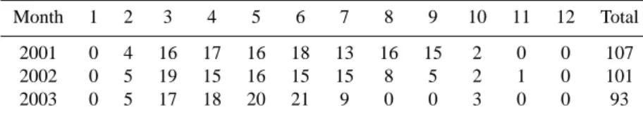
Table 2. Days of ozone observation (filter 3: 2425–3060 cm−1) from 2001 to 2003.
Month 1 2 3 4 5 6 7 8 9 10 11 12 Total 2001 0 4 16 17 16 18 13 16 15 2 0 0 107 2002 0 5 19 15 16 15 15 8 5 2 1 0 101 2003 0 5 17 18 20 21 9 0 0 3 0 0 93 Multiple measurements during a day are counted as one measurement.
Table 3. Retrieved molecules, microwindows used for retrievals, including interfering molecules, and diagonal values of Sǫand Saused in
calculations.
Molecule Microwindow [cm−1] Interfering Molecules Sǫ† Sa‡[%]
O3 3051.290–3051.900 H2O CH4 HDO CH3D 200 15
HNO3 867.450–869.250 H2O OCS 200 30 HCl 2925.800–2926.000 H2O CH4 NO2 O3 200 15
HF 4038.804–4039.148 H2O 150 15 †S
ǫis the covairance matrix of measurement noise, which is estimated from random noise in the spectral fits. ‡S
ais the covariance matrix of a priori information variability. Values are in % of mixing ratio. The same values are used for all altitudes.
(2.5 µm–13.5 µm) and 0.0019 cm−1, respectively. It uses a KCl beam splitter, and it has seven consecutive optical filters to reduce the broadband signal (avoiding detector non-linearity). The instrument is equipped with Mercury Cadmium Telluride (MCT) and Indium Antimonide (InSb) detectors, which cover the 7.0–14.0 µm and 2.0–5.5 µm spectral regions, respectively. The filters, the wavenumber ranges, the detectors, and the field-of-views used for the mea-surements are shown in Table 1. If biases coming from non-linearities of the detectors are larger than preselected thresh-old, these data is excluded in the analysis.
In order to keep the scan times for a single measurement to less than 10 min (to limit the change in airmass), the fquency resolution for the solar absorption spectrum was re-duced to 0.0035 cm−1from 0.0019 cm−1. This reduced res-olution (0.0035 cm−1) is appropriate for most studies of at-mospheric spectra in the infrared region. For example, the Doppler broadening of ozone lines is larger than 0.004 cm−1 in the 3051 cm−1region of this analysis hence a resolution of 0.0035 cm−1is adequate.
The FTS automatically observes solar absorption spectra 0–10 times a day under clear sky conditions. Since measure-ments are performed when the solar zenith angle and weather conditions are favorable (giving spectra with adequate preci-sion and noise characteristics), the number of resulting mea-surement days is about one third of the calendar year. For example, observation days for ozone (3 µm filter) were 107, 101, and 93 days for 2001, 2002, and 2003, respectively (see Table 2).
Observed spectral data are automatically transferred from computer storage at Poker Flat, Alaska to the data server in
NICT, Tokyo once every 30 min. The System for Alaska Middle-atmosphere Observation data Network (SALMON) is the means of secure and high-speed data transfer experi-ment; the network comprises a virtual private network (VPN) and the international high-speed Asia Pacific Advanced Net-work (APAN) system (Oyama et al., 2002). The netNet-work system enables the acquisition of spectral data in quasi-real time.
3 Retrieval analysis
The retrieval procedure used the SFIT2 software (version 3.7) algorithm, which incorporates Rodgers’ formulation of the Optimal Estimation Method (OEM) with an iterative Newton scheme (Rodgers, 2000). SFIT2 was developed at NASA’ s Langley Research Center (LaRC) and the National Institute of Water and Atmosphere (NIWA) (Pougatchev et al., 1995, 1996; Rinsland et al., 1998).
The retrieved height profile x is derived from Eq. (5.10) of Rodgers (2000),
xi+1= xa+ Gy([y − F(xi, b)] + Ki[xi − xa]) . (1) where x is the vector containing the profile of chemical species to be retrieved. xa is the vector of a priori vertical profiles of the chemical species to be retrieved, y is the vec-tor of the spectral measurements, and F(x, b) is the forward model calculation of the spectrum using model parameters b. The m×n matrix K = ∂F∂x is a weighting function, which is a measure of the forward model’s sensitivity to the vector of the chemical species of interest. i is an iteration number.
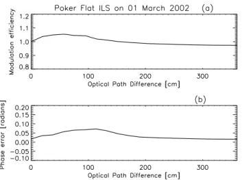
Fig. 1. (a) Retrieved modulation efficiency for Poker Flat FTS using HBr cell measurement on 1 March 2002. (b) Retrieved phase error from the same HBr cell measurement.
Gyis the contribution function matrix: Gy = SaKTi (KiSaKTi + Sǫ)
−1. (2)
where Sǫand Saare covariance matrices of the measurement noise and a priori vertical profile, respectively. The averaging kernel matrix, A, is given by
A = GyK . (3)
The parameters used in the retrieval procedure, includ-ing the frequency region, interferinclud-ing molecules, and diagonal values of the measurement noise and a priori profile covari-ance matrices (Sǫ and Sa) are listed in Table 3. We used the frequency region of ∼3051 cm−1for ozone, which is similar to the region used in Seki et al. (2002), because the tem-perature dependence of these transitions is relatively small while the only interfering molecules are the wings of two water lines. The microwindow region selected for the HCl and HF retrievals were based on similar regions from Liu et al. (1996). Diagonal elements of Sǫ were determined from typical 1-σ random noise of the spectral fits within the fit-ted spectral regions. The single value for the random noise is set for the entire fitted spectral region because variations in measurement noise within the fitted spectral regions are not significant. Non-diagonal elements of Sǫare set to zero. Non-diagonal elements of Sa are set by assuming an inter-layer correlation length of 4 km with a Gaussian distribution. The instrument line shape (ILS) function was obtained from a retrieval using a spectrum from an HBr cell measure-ment. Measurements of HBr cell spectra are performed about once every 3–6 months when there are frequent atmospheric observations and less than once a year during periods when there are less frequent observations using glow-bar source. LINEFIT9 was used for ILS retrievals (Hase et al., 1999).
Subsequent retrievals of atmospheric chemical species are performed using direct output from LINEFIT9 that includes information on the modulation efficiency and phase error de-rived from our HBr measurements. Figure 1 shows an exam-ple of derived modulation efficiency and phase error from a measurement of HBr cell spectra observed on 1 March 2002. A priori profiles were compiled from satellite data. Monthly profiles of ozone, HCl, and HF were calculated by interpo-lating on both time and vertical grids from HALOE version 19 data between 60–70◦N for the time period from 2001 to 2003. Monthly HNO3a priori profiles were computed from MLS version 5 data in 1996 using a similar method employed for ozone. The corresponding monthly a priori error covari-ance matrices, Sa, were determined from the variability of profiles within the monthly set of satellite data used to make the a priori profiles. Of the interfering molecules that af-fect the various retrieval intervals, H2O should be treated with care as it is almost always present in all microwin-dows, to varying degrees. A priori profiles of H2O were taken from rawinsonde observations made at Fairbanks ev-ery day at 15:00 AKST over the range 0–10 km and con-nected smoothly to a profile above 10 km that was based on model calculations made by the Rutherford Appleton Lab-oratory (Reburn et al., 1999). The spectral absorption line shape depends primarily on pressure, while the line strength depends primarily on temperature. Temperature and pres-sure data were also taken from the same daily 15:00 AKST rawinsonde observations at Fairbanks from 0 to 30 km, and smoothly connected to the nearest UK Meteorological Office (UKMO) point for Poker Flat from 30–50 km, and CIRA86 data for the upper region from 50–100 km (Lorenc, 2000; Swinbank and O’Neill, 1994). The spectroscopic parame-ters were taken from the High-resolution Transmission (HI-TRAN) 2004 database (Rothman et al., 2005). Retrieval height steps for all species were set using the internal grid spacing of SFIT2 and were 2 km for the first 50 km and 10 km above this to the top of the atmosphere (100 km).
4 Retrievals of O3, HNO3, HCl, and HF
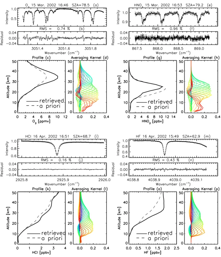
Figure 2 shows examples of the observed and calculated spectra, residuals (observed spectrum – calculated one), retrieved profiles, and averaging kernel functions for O3, HNO3, HCl, and HF. Several criteria were used to remove spectra that were outside predefined thresholds. If any spec-tra were outside these limits, this data was removed from the plot and not included in the consideration of seasonal varia-tions or correlavaria-tions. The threshold values were selected by examining plots of the root-mean-square residual and mea-surement signal to noise and/or the root-mean-square resid-ual and a second order derivative of the departure of the re-trieved profiles from the a priori profile. This eliminated noisy spectra and retrieved profiles with excessive oscilla-tions. The criteria used in this analysis were 1.5% of RMS
Fig. 2. (a) Superimposition of observed and fitted normalized spectra for ozone. Observed and calculated spectra are indicated with a cross mark and solid line, respectively. (b) Residual of these spectra. The residual is calculated by observed - calculated spectrum. (c) Ozone profiles from 0km to 50km retrieved from the spectrum of Fig. 2a. Solid line shows a retrieved profile. Long-dashed line is a priori vertical profile. (d) Averaging kernel function for the ozone mixing ratios. (e–h) are the same as (a–d), except for nitric acid. (i–l) are the same as (a–d), except for HCl. (m–p) are the same as (a–d), except for HF.
residual for ozone and 1.2% of RMS residual for HNO3, HCl, and HF. The calculated spectra (indicated with solid lines) are well fitted to the observed spectra (indicated with “x” ) in Fig. 2. The averaging kernel plot for ozone indicates that there is good information in the altitude range from 12– 35 km. Similarly, the HNO3volume mixing ratio profile has reasonable sensitivity from approximately 15 to 30 km. Both HCl and HF have similar spectral features, i.e. a single iso-lated line, and therefore their averaging kernels indicate good information from ∼12 to 35 km. The height resolutions of the retrieved profiles in the lower stratosphere, expressed as the full width at half maximum (FWHM) of individual av-eraging kernels, are about 6 km for the four species in this study.
Schneider et al. (2005b) reported ozone profiles from 1999 to 2002 observed by gb-FTS over Iza˜na Observa-tory (28.18◦N, 16.29◦W, 2370 a.s.l.) using two wavenum-ber regions centered at 782.5 and 789 cm−1. Schneider et al. (2005a) reported time series of stratospheric O3, HCl, HF, N2O and CH4from 1999. While the microwindows for ozone retrievals used by Schneider et al. (2005a, b) are dif-ferent from the intervals adopted in this study, one of the microwindows for HCl and the microwindow for HF used by Schneider et al. (2005a) are the same as those used in this study. Profiles for O3, HCl, and HF (Fig. 3 of Schneinder et al. (2005b) and Fig. 9–11 of Schneider et al. (2005a)) and their averaging kernels (Fig. 2 of Schneinder et al. (2005b) and Fig. 7 of Schneider et al. (2005a)) show similar features to this study (Fig. 2). Averaging kernels for HCl and HF from Fig. 1 of Barret et al. (2005) are consistent with ones in this study. The similar characteristics that the retrieved profiles and averaging kernels for O3, HCl, and HF show in this study with that of both Barret et al. (2005) and Schneider et al. (2005a, b) indicates that the retrievals from the spectra observed over Poker Flat are reasonable and consistent with previous studies.
Degrees of freedom for signal (DOFS) indicates the num-ber of independent pieces of information in a measurement (Rodgers, 2000), and is calculated from the trace of the av-eraging kernels matrix, A. Barret et al. (2005) obtained a number of independent partial columns by using the DOFS as a guide. They concluded that in the case of an HCl and HF measurement, one obtains two relatively independent pieces of information that can be approximated by intervals from 14–24 and 24–40 km. For this study, we used a similar proce-dure; we computed DOFS over altitude ranges to determine the best combination of intervals for the Poker Flat measure-ment system, i.e., the intervals which match the ones origi-nally obtained by Barret et al. (2005).
For ozone, Barret et al. (2002, 2003) reported a DOFS of 3.0 and 4.7 from retrievals obtained by ground-based FTS for narrow and broad microwindows, respectively. Barret et al. (2002, 2003) adopted a wide microwindow to improve the sensitivity and vertical resolution in the tropospheric re-trievals, which also reduces the dependence of the retrieval
on the a priori profiles. Typical DOFS from the microwin-dows for the ozone, HNO3, HCl, and HF retrievals used in this study are 3.0–4.0, 2.0–4.0, 2.0–3.0, and 2.0–3.0, respec-tively. The values are comparable with Barret et al. (2005, 2002, 2003) and indicate that the vertical resolution of the re-trievals from the ground-based FTS spectra used in this study is appropriate for stratospheric investigation.
5 Error analysis
5.1 Theoretical basis
The total error covariance matrix (S) can be expressed as the sum of the error covariance matrices with respect to the con-tributions from (1) the measurement error due to statistical measurement noise (SM), (2) the smoothing error, here aris-ing from the limited altitude resolution of the observation system (SN), and (3) the error due to uncertainties of non-retrieved forward model parameters (Smodel), such as spec-troscopic parameters:
S = SM + SN+ Smodel. (4)
The individual terms in Eq. (4) are: 1. measurement error covariance SM:
SM = GySǫGTy . (5)
2. smoothing error covariance SN:
SN = (A − I)Sa(A − I)T. (6)
3. model parameter error covariance Smodel:
Smodel = (GyKb)Sb(GyKb)T. (7) Sb is the error covariance matrix for the model parameter vector, and Kb is the weighting function with respect to the model parameters. In Eq. (6), to estimate SNadequately, Sa should be set to represent actual variability in the measured atmosphere. In practice, the Samatrix in SFIT2 is set as a tuning parameter, whereby the diagonal elements of the ma-trix are set to be a function related to an atmospheric variable (proportional to the mixing ratio of the target gas for exam-ple), and then scaled to give retrieved profiles that are well behaved (i.e., scaled as high as possible without introducing undue oscillations in the retrieved profile). The estimated smoothing error using this method tends to underestimate the error due to the natural variability in the atmosphere (which is a feature of most of similar studies).
5.2 Model parameters
We have estimated the random and systematic errors for the ozone, HNO3, HCl, and HF retrievals. As well as estimat-ing the errors for total columns, errors for partial columns were also computed. The altitude ranges over which the par-tial column were derived, and therefore the error estimates,
were determined on the basis of the DOFS as discussed in Sect. 4. Barret et al. (2002, 2003) selected five height in-tervals to compute their partial columns for ozone and error estimations, producing averaging kernel functions that were relatively uncorrelated, as illustrated in Fig. 3a. Connor et al. (1997) first reported the possibility of retrieving several HNO3partial columns. Figure 3b shows the averaging ker-nel functions for HNO3. In this study, we have adopted the same vertical grids for partial columns as used by Barret et al. (2002, 2003) and Connor et al. (1997) for ozone and HNO3, respectively. The grids for HCl and HF (see Sect. 4) were selected by using a DOFS that produced averaging ker-nel functions that were as uncorrelated as possible. These av-eraging kernel functions (Figs. 3c–d) show large peak values around the center altitudes of the selected layers, although the upper layer, from 20 to 40 km, does not have an obvious Gaussian tail at higher altitudes. However, the two partial columns do separate the stratosphere into two relatively in-dependent layers that give reasonable estimates of both the partial columns and their associated errors.
The total error of the retrieval consists of random and sys-tematic error components. In this analysis, the random error of the retrieval is calculated using Eqs. (5)–(7). Measurement and smoothing errors were computed using formulas (5) and (6). The model parameter temperature error was estimated as a source of non-negligible random error using Eq. (7). The contribution function for temperature was computed by sys-tematically perturbing the forward model over each height layer. SFIT2 is de-coupled from the ray-tracing algorithm, which computes airmasses as well as density-weighted tem-perature and pressure profiles. This means that computation of analytical derivatives for temperature is not possible. The temperature error covariance matrix was obtained by com-puting the standard deviation of temperature from 1 year of temperature data, which were from 1–2 to ten degrees in the lower stratosphere.
Systematic spectroscopic errors (line strength and pressure broadening parameters) and the Effective Apodization Pa-rameter (EAP) were estimated, because these errors can di-rectly affect retrieved profiles (Barret et al., 2002, 2003; Park, 1982). A simple method of perturbation was used whereby the departure of the retrieved profile with a modified model parameter is calculated from one with an unchanged param-eter using Eq. (8).
1xmodel = Gy[F(x, b + 1b) − F(x, b)] . (8) Here, 1b is the uncertainty in the model parameter to be investigated. We assumed uncertainties of 5% higher line strength and 10% smaller air-broadening coefficient in the HITRAN 2004 spectroscopic parameters, on the basis of val-ues described in the error flags of the HITRAN database. The synthesized spectra were therefore calculated with line inten-sities of all target molecules in the retrieval ranges multiplied by 1.05. These synthesized spectra were then retrieved with unperturbed spectroscopic parameters, as Barret et al. (2002,
Fig. 3. (a) Averaging kernel functions for partial columns of ozone. Averaging kernel functions for 0–12, 12–18, 18–24, and 24–40 km are shown as independent layers. The total column is also indicated as a solid line. (b), (c), and (d) are plots of HNO3, HCl, and HF,
respectively. The averaging kernels are calculated using the same spectra used for Fig. 2.
2003) did. The same procedure was used for the estimation of error in the air broadening coefficient uncertainty of the target species. The synthesized spectra were calculated with the air-broadening coefficients of all the target molecules in the retrieval ranges multiplied by 0.90 and retrieved with un-perturbed parameters. A 10% uncertainty was assumed for the EAP, which is consistent with recent practice (Barret et al., 2002, 2003; Nakajima et al., 1997). The error due to the uncertainty in EAP was calculated with the same method as was used for the spectroscopic parameters. Synthesized spectra were computed with an EAP of 0.9 (i.e., modulation efficiency is set to 0.9 at the maximum path difference in the FTS), and then retrieved with an assumed EAP of 1.0. 5.3 Results of error analysis
The results of the error analysis are detailed in Table 4. Twenty measurements were randomly selected, one per month, from 2001 to 2003 to estimate the errors. All error estimates in Table 4 are averages over the 20 randomly se-lected days. Total random error was calculated as the
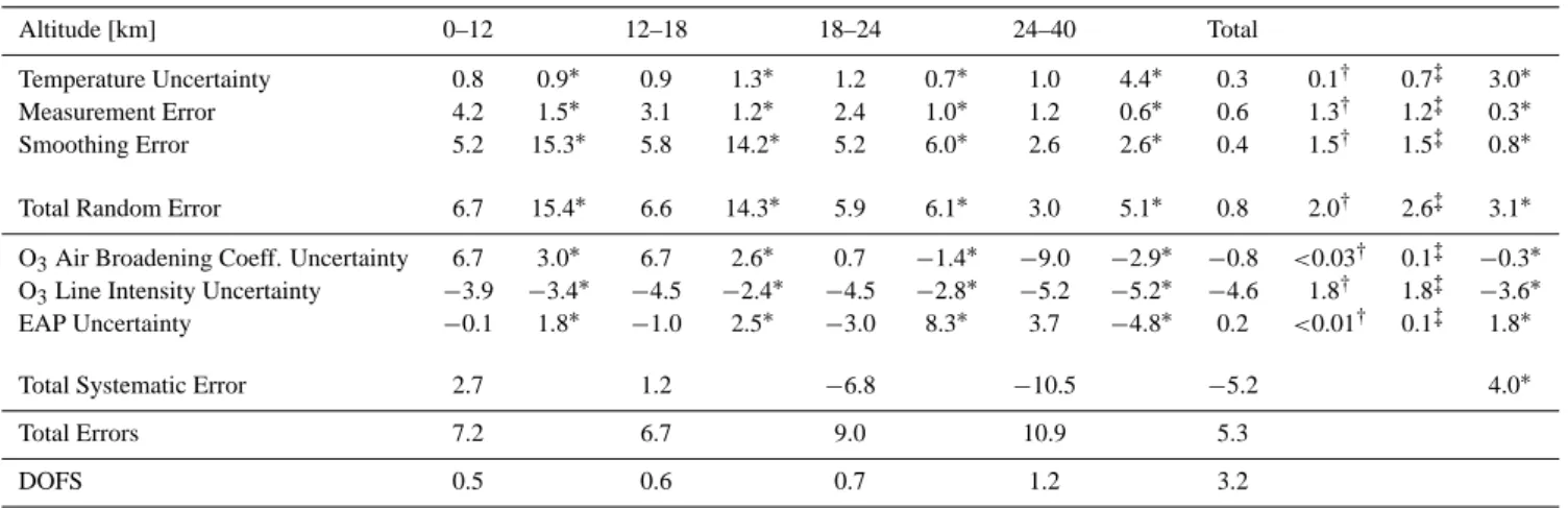
root-Table 4a. Errors in ozone for 0–12, 12–18, 18–24, 24–40 km partial columns and for the total column. All errors are in % of the column amount. DOFS of these partial columns and total column are also indicated.
Altitude [km] 0–12 12–18 18–24 24–40 Total
Temperature Uncertainty 0.8 0.9∗ 0.9 1.3∗ 1.2 0.7∗ 1.0 4.4∗ 0.3 0.1† 0.7‡ 3.0∗
Measurement Error 4.2 1.5∗ 3.1 1.2∗ 2.4 1.0∗ 1.2 0.6∗ 0.6 1.3† 1.2‡ 0.3∗
Smoothing Error 5.2 15.3∗ 5.8 14.2∗ 5.2 6.0∗ 2.6 2.6∗ 0.4 1.5† 1.5‡ 0.8∗
Total Random Error 6.7 15.4∗ 6.6 14.3∗ 5.9 6.1∗ 3.0 5.1∗ 0.8 2.0† 2.6‡ 3.1∗
O3Air Broadening Coeff. Uncertainty 6.7 3.0∗ 6.7 2.6∗ 0.7 −1.4∗ −9.0 −2.9∗ −0.8 <0.03† 0.1‡ −0.3∗
O3Line Intensity Uncertainty −3.9 −3.4∗ −4.5 −2.4∗ −4.5 −2.8∗ −5.2 −5.2∗ −4.6 1.8† 1.8‡ −3.6∗
EAP Uncertainty −0.1 1.8∗ −1.0 2.5∗ −3.0 8.3∗ 3.7 −4.8∗ 0.2 <0.01† 0.1‡ 1.8∗
Total Systematic Error 2.7 1.2 −6.8 −10.5 −5.2 4.0∗
Total Errors 7.2 6.7 9.0 10.9 5.3
DOFS 0.5 0.6 0.7 1.2 3.2
A 5% larger line intensity and 10% smaller air-broadening coefficient than those of HITRAN 2004 are assumed for the spectroscopic error.
†Error for total column by Schneider et al. (2005b) ‡Error for total column by Schneider et al. (2005a)
∗Total and partial column errors for narrow window by Barret et al. (2002, 2003)
Table 4b. Error in HNO3.
Altitude [km] 10–20 20–30 Total Col.
Temperature Uncertainty 0.9 0.8 0.5 1.2† Measurement Error 5.7 4.2 2.5 2.0† Smoothing Error 9.5 6.4 2.1 2.0† Total Random Error 11.1 7.7 3.3
HNO3Air Broadening Coefficient Uncertainty 2.7 −1.6 3.4
HNO3Line Intensity Uncertainty −4.7 −5.1 −4.4 ∼10.0†∗
EAP Uncertainty −1.1 1.0 0.0 Total Systematic Error −3.1 −5.7 −1.0
Total Errors 11.5 9.6 3.4
DOFS 0.7 1.1 2.6
†Error for total column by Wood et al. (2004) ∗The value is for line parameter uncertainty.
sum-square of the temperature uncertainty, measurement er-ror, and smoothing error. Total systematic errors were calcu-lated as the sum of spectroscopic error and EAP uncertain-ties.
The errors for the total column and for the partial columns (0–12, 12–18, 18–24, 24–40 km) for ozone were 5.3, 7.2, 6.7, 9.0, and 10.9%, respectively, as recorded in Table 4a. Among the estimated error elements, the impact of temperature un-certainty is small for all the columns. Systematic errors for total and partial columns were −5.2 and −10.5–2.7%,
re-spectively, and these have large variations depending on the partial column.
Barret et al. (2002, 2003), as mentioned, estimated the ozone error by using a similar method to this study. Since this study’s error estimates are comparable to the ones reported by Barret et al. (2002, 2003) for the narrow window cases, their errors for total and partial columns have been included in the Table 4a for comparison purposes (values with asterisk symbols). Our errors for the ozone total and partial column are consistent with Barret et al. (2002, 2003) as shown in the
Table 4c. Error in HCl.
Altitude [km] 10–20 20–40 Total Col. Temperature Uncertainty 0.6 0.5 0.4 1.0† Measurement Error 3.2 1.7 1.2 1.2† Smoothing Error 3.6 2.7 1.4 1.1† Total Random Error 4.9 3.3 1.9 2.2† HCl Air Broadening Coefficient Uncertainty 3.1 −7.3 −1.7 0.6† HCl Line Intensity Uncertainty −4.2 −5.3 −4.0 4.3† EAP Uncertainty −1.4 1.8 0.1 0.1† Total Systematic Error −2.5 −10.8 −5.6
Total Errors 5.5 11.3 5.9 2.7∗
DOFS 0.8 1.2 2.1
†Error for total column by Schneider et al. (2005a) ∗Error for total column by Barret et al. (2005)
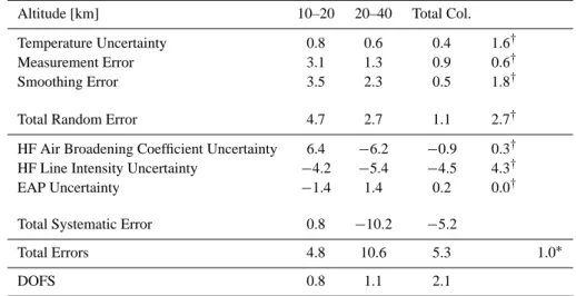
Table 4d. Error in HF.
Altitude [km] 10–20 20–40 Total Col. Temperature Uncertainty 0.8 0.6 0.4 1.6† Measurement Error 3.1 1.3 0.9 0.6† Smoothing Error 3.5 2.3 0.5 1.8† Total Random Error 4.7 2.7 1.1 2.7† HF Air Broadening Coefficient Uncertainty 6.4 −6.2 −0.9 0.3† HF Line Intensity Uncertainty −4.2 −5.4 −4.5 4.3† EAP Uncertainty −1.4 1.4 0.2 0.0† Total Systematic Error 0.8 −10.2 −5.2
Total Errors 4.8 10.6 5.3 1.0∗
DOFS 0.8 1.1 2.1
†Error for total column by Schneider et al. (2005a) ∗Error for total column by Barret et al. (2005)
table. The smoothing error in the two layers below 18 km in this study have smaller values than the comparable smooth-ing errors in the Barret et al. (2002, 2003) studies. This may be due to differences in the assumed conditions for the error calculations.
Schneider et al. (2005a, 2005b) reported a detailed error analysis also using a similar method to this study. Calcula-tions of ozone total errors by Schneider et al. (2005a, 2005b) are included in Table 4a (value with dagger symbols). Their error values are also consistent to this study although there
are slight differences which, like the Barret et al. (2002, 2003) studies, possibly come from assumptions in the error calculations and selection of spectra. Overall consistency of error values calculated in this study with Barret et al. (2002, 2003) and Schneider et al. (2005a, 2005b) indicate that the ozone retrieval process of this study is consistent with previ-ous published reports.
Fig. 4. (a) (left) Comparison of ozone profiles measured by FTS with colocated ozonesonde measurements from 0 to 50 km. The solid blue line shows a retrieved ozone profile on 22 March 2001 18:00 UTC. The dash-dotted sky-blue line is the a priori profile used for this retrieval. The dotted red line shows a profile observed by an ozonesonde launched from Fairbanks (64.81◦N, 147.86◦W) on 22 March 2001 18:26 UTC. The pink solid line shows an ozonesonde profile smoothed using the FTS averaging kernel. The time difference between the ozonesonde and FTS measurements is indicated in the figure (ozonesonde observation time - FTS observation time). (middle) Red long-dashed line is the relative difference between the original ozonesonde and FTS ozone as calculated by 100×(O3(FTS)-O3(sonde))/O3(sonde). The pink line is the relative difference between the smoothed ozonesonde and FTS ozone calculated with the same method as the original ozonesonde difference above. (right) An averaging kernel function for the FTS measurement of (a) which is used to smooth the ozonesonde profile. (b–d) are the same as (a), except for the measurements by FTS and ozonesonde on 23 March, 24 March, and 25 April.
The total HNO3 errors for the total column, 10–20, and 20–30 km partial columns, are 3.4, 11.5, and 9.6%, respec-tively (Table 4b). The results of an error analysis of the total column HNO3 by Wood et al. (2004) are included in Table 4b (values with dagger symbols). Their error values compare well with values in this study. A random error of 3.6% was estimated by Rinsland et al. (2000) for both the 14–20 km and 20–50 km HNO3partial columns. Systematic errors were reported as 11.4 and 14.2% for the 14–20 km and 20–50 km partial columns, respectively. A direct compari-son of the errors from this study with those of Rinsland et al. (2000) is difficult due to differences in the methods used to estimate the errors; however, the error budgets for HNO3 are consistent between these studies.
The error budgets for HCl and HF are shown in Tables 4c and d. The total HCl errors for the total column, 10–20, and 20–40 km partial columns are 5.9, 5.5, and 11.3%, re-spectively. The respective total HF errors for the total col-umn, 10–20, and 20–40 km partial columns are 5.3, 4.8, and 10.6%, respectively. Although the total errors of the total column for HCl and HF are slightly higher than the values reported by Barret et al. (2005) as shown in Table 4c and d (value with asterisk symbols), the error estimates from their work and our study are consistent. Errors reported by Schnei-der et al. (2005a) are also shown with dagger symbols in Ta-ble 4c and d, which are also quite consistent with these errors in this study.
When the error budgets for all the reported species are considered, the systematic errors are larger than random er-rors. Uncertainties in the spectroscopic parameters have the largest impact on the total error. This reflects the direct influ-ence that these types of error have on the spectral line shape in the retrieval process. Similar features in the error analyses from this work are also reported by Barret et al. (2002, 2003), Rinsland et al. (2000), Schneider et al. (2005a, b), and Wood et al. (2004).
Schneider et al. (2005a, b) reported in their detailed error analysis that the phase error that results from a non-perfect ILS is not negligible; the error is within ∼1% for the total and partial ozone columns for ozone, HCl, and HF except for HCl in the troposphere column. Therefore, inclusion of an ILS phase error could possibly result in a slightly different estimation of systematic error in this study.
In summary, the total errors are within 5.9% for the total column, and 11.5% for the partial columns from the Poker Flat ground-based FTS measurements of stratospheric O3, HNO3, HCl, and HF. These errors are consistent with error budgets reported in previous FTS measurements from other NDACC sites.
6 Validation
6.1 Comparison of FTS O3and ozonesonde data
In this section, we validate retrieved ozone data from the gb-FTS measurements by comparison with ozonesonde data. Figure 4 compares the FTS retrieved ozone profiles and ozonesonde profiles. Ozonesonde measurements were per-formed as a part of the TOMS3-F campaign in Fairbanks (64.81◦N, 147.86◦W; ∼40 km southwest of Poker Flat) dur-ing the sprdur-ing of 2001, in which 28 profiles were obtained from 20 March to 25 April. The reported error in the ozone profiles from the ozonesonde was approximately 5% (Komhyr et al., 1995).
Profiles whose observation time was within 12 h of the ozonesonde observation time were selected from the FTS measurement during spring 2001. There were 11 FTIR pro-files that had ozonesonde counterparts, whereas there were 2 FTIR profiles with residual root mean squares larger than 1.0%, which indicated a small oscillation in the lower strato-sphere, and hence, these two profiles were discarded from the comparison. There were 13 comparisons between FTS and ozonesonde using 9 FTS profiles for 5 days (some FTS profiles had multiple ozonesonde profiles for comparison): 22 March (2 cases), 23 March (6 cases), 24 March (2 cases), 24 April (1 case), and 25 April (2cases) 2001. Figures 4a–d compare minimum time differences for the 22, 23, and 24 March, and 25 April 2001.
When comparing two different measurement techniques that are measuring a similar geophysical quantity, care should be taken when evaluating the two observation
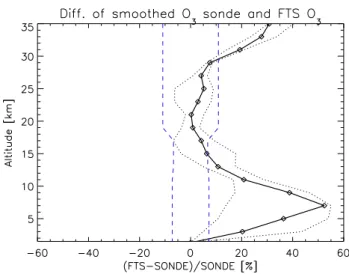
sys-Fig. 5. Difference between ozonesonde ozone profiles observed in Fairbanks (64.81◦N, 147.86◦W; ∼40 km southwest of Poker Flat) and FTS ozone profiles during the spring of 2001. FTS observa-tions whose RMS residuals are smaller than 1% and observation time is within 12 h of the ozonesonde observations were selected for the comparison. Open diamond with solid line shows the me-dian of the relative differences calculated from the 13 comparisons selected according to the criteria. Black dotted lines are the 25 and 75 percentile values. Blue dashed line is the FTS error range of the partial column calculated by the error analysis at the corresponding altitude.
tems (for example comparing an FTS with ozonesonde pro-files). In particular, the characteristics of how the measuring systems sample the atmosphere must be taken into account through the use of averaging kernel functions (Rodgers and Connor, 2003). In this study therefore, the profiles observed by the ozonesondes were smoothed with the FTS averaging kernels and these modified ozonesonde profiles were com-pared with the ozone profiles derived from the FTS. The smoothing procedure is reported in an earlier paper (Ya-mamori et al., 2006).
Figure 4 compares the smoothed profiles of ozonesonde ozone (pink lines) with FTS ozone profiles. The smoothed profiles have much better agreement with the FTS profiles particularly in the left panels (profile comparison) of Figs. 4b and c for the lower and middle stratosphere.
The percentage differences between FTS ozone and ozonesonde ozone were calculated for 13 comparisons using 100×(O3(FTS)-O3(sonde))/O3(sonde)%. Figure 5 shows median, 25 percentile, and 75 percentile values of the dif-ferences. The blue dashed lines are computed error ranges for the partial columns. From 15 to 30 km, the median of the difference is within the error range of the FTS partial column. There is about a 50% median difference with large scatter at 7 km. This large difference is caused by a combination of limited sensitivity from the retrieval (as the averaging ker-nel rapidly falls off around this altitude), and the effect this
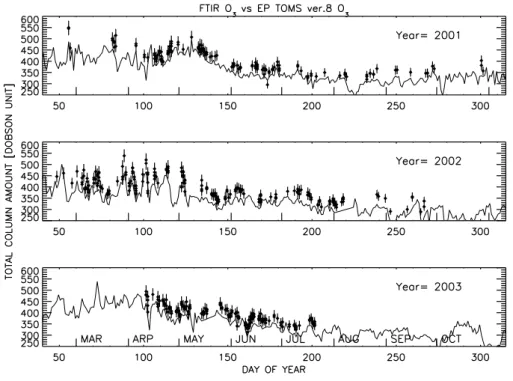
Fig. 6. Comparison of FTS ozone and Earth-Probe TOMS data. Filled diamonds with error bars indicate FTS ozone. The error bar for the FTS ozone data is taken from the total error as computed in the error analysis. The solid line is EP-TOMS data over Poker Flat.
has on our choice of the a priori profile in the troposphere. This problem is further exacerbated by the rapid spatial (ver-tical) and temporal change in ozone mixing at and below the tropopause. Note that the error inherent in a profile is larger than the error in a partial column and that the error in the ozonesonde profile is not considered in the error ranges that Schneider et al. (2005b) included.
Schneider et al. (2005b) reported a detailed statistical com-parison between ozone derived from an FTS and smoothed ozonesondes and showed the differences were within ∼8% below 50 km. Barret et al. (2002, 2003) reported a relative difference of (FTS-sonde)/sonde for a narrow spectral mi-crowindow as 0–10% below 30 km depending on altitudes (Fig. 8 in Barret et al. (2002)). While the differences between the ozone derived from an FTS and smoothed ozonesondes as reported by Barret et al. (2002, 2003) and Schneider et al. (2005b) are consistent with values from this study in the stratosphere, this is not the case in the troposphere, where the differences in this study are larger. This difference may be due to the selection of the microwindows used in this study that results in less sensitivity to ozone at these lower alti-tudes.
Generally, the consistency of the profiles (gb-FTS and ozonesonde) in the lower and middle stratosphere, where most of the ozone exists, verifies that the observations by the Poker Flat FTS and retrieval method for ozone is compara-ble with previously reported work (Barret et al., 2002, 2003; Schneider et al., 2005b). Inclusion of additional
microwin-dows in the ozone analysis to improve sensitivity of spectra in the troposphere as Barret et al. (2002, 2003) reported is planned in the near future.
6.2 Comparison of FTS O3and TOMS data
Figure 6 compares the ozone total column from the FTS and Earth-Probe Total Ozone Mapping Spectrometer (TOMS) version 8 data from 2001 to 2003. The FTS retrieved ozone total column is shown with error bars estimated from the er-ror analysis in Sect. 5 (5.3%). The FTS and EP-TOMS mea-surements are consistent in terms of seasonal trends; how-ever, there is a uniform small negative bias in the EP TOMS data. The time series of the two data sets does show similar small-scale features on time scales of several tens of days.
One factor that explains some of this bias concerns a calibration error in TOMS. As reported in TOMS News (http://toms.gsfc.nasa.gov/news/news.html), there is a −2% to −4% error in TOMS at 50 degrees latitude, with the bias being slightly higher in the northern hemisphere than in the southern hemisphere. There is no indication in the literature of this bias error at 65◦N, but if a 5% bias in TOMS is as-sumed, the resultant difference between FTS and TOMS data is reduced as shown by the blue symbols in Fig. 7, with many data points coming within the error range of the one-to-one line. The blue solid line in Fig. 7 is the fitted line when a 5% bias in TOMS is assumed (blue symbols). The subse-quent slope and intercept of the fitted line are 0.95 and 36.9, respectively.
Another factor that explains some of this bias is from the limitation from the gb-FTS retrieved ozone volume mixing ratio in the troposphere. The sensitivity of the retrievals is not sufficient in the troposphere where about 10% of the total ozone column exists at mid-latitudes. The degree of freedom of ∼0.5 in the troposphere as reported in Table 4a indicates that this low sensitivity to tropospheric ozone is possibly a source of non-negligible bias in the total column amount. When the a priori profiles in the troposphere were changed to an averaged ozonesonde data that was used for the com-parsion in Sect. 6.1 to calculate biases of the a priori profiles used in this analysis, the retrieved total ozone columns de-creased typically by about 1.5% of the original one. While the calculation indicates that the biases of the original a priori profiles are not significant, the magnitudes are not enough to explain the differences between TOMS and FTS data.
The large departures from this one-to-one line that still remain are possibly explained by spectroscopic uncertain-ties. Using the HITRAN 2004 spectroscopic parameters for the FTS retrieval instead of HITRAN 2000 introduces sys-tematic differences between the FTS retrieved ozone and EP-TOMS data. The five strongest lines (intensities) of ozone in the retrieval microwindow from the HITRAN 2004 data (3051.3800, 3051.8307, 3051.4742, 3051.7555, and 3051.3068 cm−1) are about 4% lower than the respective HI-TRAN 2000 lines. Large differences in the air broadening coefficient and temperature dependencies of the half widths between HITRAN 2004 and the earlier HITRAN 2000 val-ues were reported by Rinsland et al. (2003a). Differences of up to 10% exist in the broadening coefficients of the two HITRAN databases. If these discrepancies are considered, the uncertainties in the spectroscopic parameters are poten-tially one of the largest error sources in the budget analysis of Sect. 5. If an additional ∼5% large bias is assumed for the spectroscopic line strength in HITRAN 2004, almost all the data now falls within the error range of the one-to-one line (Fig. 7).
6.3 Comparison of FTS O3, HCl, and HF with HALOE data
In this section, we compare stratospheric columns of O3, HCl, and HF derived from measurements made by the HALogen Occultation Experiment (HALOE) onboard the UARS satellite with data from the gb-FTS measurements. An overview of HALOE observations is given in Russell III et al. (1993). Errors in HALOE-derived O3were reported to be 8–30% from 1 to 100 hPa, and thus, the HALOE O3data are within the error range of correlative measurements (Bruhl et al., 1996). The total error for the HALOE HCl columns was reported to be from 12–24% throughout the stratosphere (Russell III et al., 1996b). Russell III et al. (1996b) reported that HALOE HCl measurements tend to be low (from 8 to 20%) in correlative comparisons with other instruments. To-tal errors for HALOE HF are reported to be 14–27%,
depend-Fig. 7. Scatter plot of EP-TOMS data with FTS total ozone column. Black x’s are the scatter plot of EP-TOMS and FTS ozone. The blue symbols are the same comparison of x but a 5% bias from the TOMS data is included. The solid line is the one-to-one line. The error range for the FTS total column ozone is also shown. The blue solid line is fitted line when a 5% bias of the TOMS data is assumed.
ing on the altitude in the stratosphere (1–100 hPa) (Russell III et al., 1996a).
Figure 8 shows stratospheric columns (15 to 49 km) of ozone, HCl, and HF for gb-FTS and HALOE version 19 over the time period from 2001 to 2003. The error ranges of the FTS O3, HCl, and HF partial columns in Fig. 8 are the ones for altitude ranges 18–24, 20–40, and 20–40 km, re-spectively. Plotted are HALOE data within 10◦latitude and 20◦longitude of Poker Flat. HALOE data from this selected area roughly correspond to the Alaskan location. HALOE data has been smoothed by the FTS averaging kernel using the same method as described for the ozonesonde compari-son in Sect. 6.1 to give a reacompari-sonable comparicompari-son. Time series of the chemical species from smoothed-HALOE and the gb-FTS were fitted using functions that include a seasonal cycle and annual trend term as shown in the figure. The seasonal variation of the smoothed-HALOE and FTS ozone, HCl, and HF columns are reasonably consistent for the 2001–2003 pe-riod, although the FTS O3and HCl are uniformly higher than the smoothed-HALOE data.
For a detailed comparison, Fig. 9 shows scatter plots of ozone, HCl, and HF columns for the smoothed-HALOE and FTS datasets measured on the same day for the 2001– 2003 time period. The FTS O3 columns, Fig. 9a, corre-late well with smoothed-HALOE data (r=0.92). Average relative differences calculated with the relation (O3
(FTS)-Fig. 8. (a) Comparison of stratospheric columns of FTS ozone and HALOE version 19 ozone from 2001 to 2003. The diamonds symbol with error bars indicates the FTS stratospheric ozone column. The FTS ozone error bars are taken from the 18–24 km partial column error (9.0%) estimated by the error analysis in Sect. 5.3. Red asterisk is the HALOE measurement smoothed by the FTS averaging kernels. HALOE data within 10◦latitude and 20◦longitude of Poker Flat is plotted. Both the FTS and HALOE data are fitted using a function that includes terms for the seasonal cycle and annual trend. (b–c) are the same as (a) except for HCl, and HF. The error bars of the FTS derived HCl and HF are for the 20–40 km columns (11.3 and 10.6 %), respectively.
O3(HALOE))/O3(HALOE) are about 10%. McHugh et al. (2005) reported FTS ozone measurements of the At-mospheric Chemistry Experiments (ACE) that were about 0.4 ppmv larger than those of the HALOE version 19 de-rived ozone mixing ratio in the altitude range from 35 to 70 km. This study’s comparison of smoothed-HALOE and gb-FTS data indicated a similar bias. If the bias of McHugh et al. (2005) is considered, most of the measurements fall within the indicated error ranges in Fig. 9a.
Figure 9b shows the FTS HCl correlation plot with smoothed-HALOE from 2001 to 2003, and this plot also indicates a positive bias for the FTS data. The smoothed-HALOE–FTS correlation (r=0.36) is lower than ozone (r=0.92) as ozone is driven by a much larger seasonal cycle. In a similar fashion to ozone, the average rel-ative difference for HCl, calculated as (HCl(FTS)-HCl(HALOE))/HCl(HALOE), is again about 8%. A simi-lar bias between HALOE data and correlative measurements was reported by Russell III et al. (1996b). Liu et al. (1996) reported that HCl profiles from gb-FTS agree with HALOE data within the combined error limit, but are 5 to 20% higher than the HALOE values. McHugh et al. (2005) also reported that ACE-FTS HCl values are 10–20% higher than those of HALOE version 19 between 20 and 48 km.
In Fig. 9c, the HF columns measured by FTS are 4% larger than those of smoothed-HALOE HF. The ACE–FTS derived HF profiles indicate 10–20% larger values than HALOE profiles throughout the stratosphere (McHugh et al., 2005). There is a moderate correlation (r=0.63) between the two measurements.
Overall, the gb-FTS O3, HCl, and HF stratospheric columns show moderate correlations with smoothed-HALOE version 19 columns but are about 4–10% higher than the HALOE version 19 columns. However, the two measurements are consistent if the bias reported by Russell III et al. (1996b), Liu et al. (1996), and McHugh et al. (2005) is considered. The two measurements, Poker Flat FTS and HALOE, will be compared in the future after HALOE data has been updated with the new version (McHugh et al., 2005).
7 Seasonal variations of O3, HNO3, HCl, and HF from
2001 to 2003
Figures 10a–d are time-height cross sections (upper panel) and the columns (lower panel, see Fig. 10 caption for de-tails) of O3, HNO3, HCl, and HF from 2001 to 2003. The
height-time cross sections are plotted for the altitude range from 10–50 km, where the chemical species were retrieved with good vertical information. Blank areas represent either no measurement or data that were rejected on the basis of quality control criteria (for example, signal to noise ratio). Intensive measurements are made from spring to autumn by the Poker Flat FTS system every year, whereas few measure-ments or few data with high enough precision are gathered during winter when the solar zenith angle is large (sun at or below the horizon). The profiles selected to produce Fig. 10 comprised 210, 160, 228, and 194 profiles for ozone, HNO3, HCl, and HF, respectively.
Despite the limited vertical resolution inherent in the FTS profiles, the retrieved profiles do exhibit seasonally varying features for the chemical species selected in this study. In the upper panel of Fig. 10a, the ozone mixing ratio over Poker Flat shows large seasonal variations, with the maximum ratio occurring around 38 km as expected. Low ozone mixing ra-tios, indicated in purple at low altitudes, gradually ascend to-wards the end of the season. Ozone total columns (the black diamonds in the lower panel of Fig. 10a) have a seasonal de-pendence, with their maximum value occurring in late winter or spring and minimum in summer. The time series of the ozone partial columns indicate that the seasonal cycle ob-served in the total column is mainly driven by changes in the lower stratosphere (12–18 and 18–24 km), with less seasonal dependence in the 0–12 km and 24–40 km partial columns. The largest seasonal change in ozone mixing ratio occurs at altitudes different from the ones where the largest seasonal change in the column happens, which is expected for ozone. Figure 10b is the retrieved time-height cross-section and columns for HNO3. The maximum mixing ratio for HNO3 occurs in the lower stratosphere, as expected. Year-to-year variability of the HNO3 total column is larger than that of ozone. The high abundance for the HNO3 total col-umn of around 3×10¹⁶molecules cm−2 in spring gradually decreases towards summer and increases again in autumn. This is consistent with summer photodissociation. Seasonal changes in the HNO3column occur at 10–20 km range, as shown by the blue symbols in Fig. 10b, with notable changes occurring in the spring of 2002. The increase in the HNO3 total column during the fall of 2001 appears to be driven by changes occurring at 20–30 km. As in the case of ozone, the altitude regions with the largest seasonal changes in mixing ratio are different from the altitudes of the largest changes in the HNO3columns.
Figures 10c and d are the retrieved time-height cross-section (upper panel) and columns (lower panel) for HCl and HF, respectively. The mixing ratio profiles of these two species have similar shapes; that is, these mixing ratios grad-ually increase with altitude from the stratosphere to higher altitudes. Both HCl and HF have similar seasonal cycles to those of O3and HNO3over the time period of the data (2001 to 2003). These seasonal cycles in HCl and HF occur in the 10–20 km range as shown in the figures. HF has a larger
Fig. 9. (a) Scatter plot of smoothed-HALOE and FTS ozone for the data displayed in Fig. 8a. Data for same-day measurements are plotted. (b–c) are the same as (a), except for HCl and HF.
Fig. 10. (a) (upper panel) Time-height cross-section of ozone mixing ratio 10–50 km over Poker Flat from 2001 to 2003. The ozone mixing ratio scale is indicated with accompanying color bar. Data are plotted only for the period when observations and data retrieval were of sufficient quality and precision. When multiple observations were made on a single day, the observation nearest 15:00 (AKST) is selected for the plot which is the time at which the local sonde is flown and hence the source of the temperature data used in the FTS retrieval. (Lower panel) Black: Ozone total column for the same data as the upper panel. Blue: Ozone partial column for 0–12 km. Green: Ozone partial column for 12–18 km. Yellow: Ozone partial column for 18–24 km. Red: Ozone partial column for 24–40 km. (b) (upper panel) same as (a), except for HNO3. (lower panel) Black: HNO3total column. Blue: HNO3partial column for 10–20 km. Red: HNO3partial column
for 20–30 km. (c–d) (upper panels) same as (a), except for HCl or HF. (lower panels) Black: HCl and HF total column. Blue: HCl and HF partial column for 10–20 km. Red: HCl and HF partial column for 20–40 km.
Fig. 11. (a) Asterisk: Time series of Potential Vorticity over Poker Flat at 475 K in 2001. Solid line: Potential Vorticity at Vortex edge. Dotted lines: Potential Vorticity at the poleward (inner) and the equatorward (outer) edge of vortex boundary region calculated using method of Nash et al. (1996). Vortex edges are plotted only for periods when Polar Vortex exists. PV is calculated using UKMO data. (b) same as (a) except for 2002 data. (c) same as (a) except for 2003 data.
partial column at 20–40 km (red symbols) than at 10–20 km (blue symbols). There are also possible dynamical features in the 10–20 km column, particularly for HF, that are also ap-parent in the HNO310–20 km column. This is quite clear for the 2002 data.
To investigate the dynamical features, Fig. 11 shows time series of Potential Vorticity (PV) at 475 K over Poker Flat (asterisks), PV at vortex edge (solid lines), PV at the pole-ward (inner) edge of vortex boundary region (dotted lines), and PV at the equatorward (outer) edge of vortex boundary region (dotted lines) calculated based on UKMO meteoro-logical data using the method of Nash et al. (1996). Fig-ure 11 shows that all the observations over Poker Flat were made outside the vortex in the late winter and spring of 2001– 2003, as there were no observations taken when Poker Flat was located inside the vortex with the exception of several days in late March 2003 (day number is around 87 in Fig.11).
Figure 11 suggests that the chemical species observed over Poker Flat were not influenced by polar chemistry over these periods. However, the consistently large enhancement of all species studied in the lower stratosphere for the period in mid-April in 2002 (Fig. 10) and the period around the vor-tex breakup at approximately day number 103 in Fig. 11b suggests the possible influence of the vortex on these chem-ical species. A detailed daily comparison of PV and various chemical species is the subject of a current study.
The difference between retrievals that used monthly a pri-ori profiles and a single a pripri-ori profile for all four species was checked to investigate the influence of different a priori profiles on observed seasonal changes (Fig. 10). The calcula-tion indicated that the seasonal cycles in the total and partial columns observed in Fig. 10 can be attributed to changes in the real atmosphere for all four retrieved species. This is due to the fact that similar seasonal cycles were calculated using
a single a priori profile, even for the specific cases of partial columns.
The magnitudes of the seasonal cycles in the total and par-tial columns derived from Fig. 10 for all species were com-pared with their respective error ranges reported in Table 4. In all cases except one, the magnitudes of the seasonal cy-cles for both the total and partial columns exceeded their tab-ulated errors. Specifically, the total column seasonal cycle magnitudes (an partial column in brackets) for O3, HNO3, HCl, and HF were 17% (4–38), 37% (33–60), 13% (10–33), and 18% (6–51%) respectively. The exception was the 24– 40 km partial column for ozone.
8 Summary
We have been observing stratospheric minor species over Poker Flat, Alaska since 1999 by using a high-resolution FTS. Poker Flat is at an interesting location between the Arc-tic and mid-latitudes. To investigate the behavior of strato-spheric ozone and ozone-related species, vertical profiles of ozone, HNO3, HCl, and HF for the period of 2001–2003 were retrieved using Rodgers’ formulation of the Optimal Estimation Method (OEM). The averaging kernel functions indicated that the four chemical species were retrieved with the highest information content in the lower stratosphere. Due to the limited vertical resolution inherent in gb-FTS measurements, there are only 2 to 4 relatively independent partial columns that can be investigated, depending on gas species.
The retrieval errors were estimated in detail and used as the basis for discussion of seasonal and inter-annual variabil-ity in stratospheric ozone and ozone-related species. The ran-dom and systematic errors of the retrieved partial column of the chemical species were calculated by formal error analy-sis. The total ozone errors for the total column and 4 partial independent columns are 5.3% and 6.7–10.9%, respectively. Similarly, the total errors for the HNO3, HCl, and HF total columns were 3.4, 5.9, and 5.3% respectively, while the total errors for the reported two partial columns of HNO3, HCl, and HF were 9.6–11.5, 5.5–11.3, and 4.8–10.6% , respec-tively. These errors are consistent with previous error bud-gets of the FTS measurements reported from other NDACC sites. In our analysis, line parameters and EAP uncertainties were significant components of the total error.
We validated the data retrieved from our FTS measure-ments by comparison with ozonesonde, Earth-Probe TOMS, and HALOE data. For consistency with current best practice, the ozonesonde profiles were smoothed by the FTS averaging kernel functions. These smoothed profiles agreed well with the FTS ozone profiles within their calculated error ranges of 15–30 km where FTS has sensitivity. The total column ozone observed by the FTS and EP-TOMS version 8 were consis-tent within the FTS error bars if the known systematic bias in the EP-TOMS data and HITRAN 2004 is taken into account.
Stratospheric columns of ozone, HCl, and HF observed by the FTS were compared with HALOE version 19 data. HALOE data were smoothed by the FTS averaging kernel functions. The FTS O3, HCl, and HF stratospheric columns were moderately correlated with smoothed-HALOE data but were about 4–10% high. However, the two measurements are consistent when the biases reported by other studies are taken into account. A new version of HALOE has been developed, and we will compare the two measurements again by using the updated data (McHugh et al., 2005). FTS HNO3profiles during the 2003 spring agreed well with the Improved Limb Atmospheric Spectrometer (ILAS) II data (Yamamori et al., 2006).
Of the height-time cross-sections of the chemical species retrieved by FTS in this study, the ozone data from 2001– 2003 exhibited a seasonal cycle with its maximum mixing ratio being in the mid-stratosphere. HNO3 also exhibits a seasonal cycle with its maximum mixing ratio being in the lower stratosphere. All four retrieved species had similar seasonal cycles, and seasonal variations in the columns of all species occurred in the lower stratosphere. All the obser-vations over Poker Flat were made outside the polar vortex in the late winter and spring of 2001–2003.
This study is the first report of retrieval results with a de-tailed formal error analysis of stratospheric molecules above the Poker Flat FTS observation site. A further investiga-tion of the ozone loss mechanisms over Poker Flat will be reported in the near future.
Acknowledgements. The authors thank the United Kingdom
Me-teorological Office (UKMO) for supplying temperature, pressure, and wind data for the retrievals and PV calculations. We are grate-ful to NASA’s Goddard Space Flight Center for providing Total Ozone Mapping Spectrometer (TOMS) data from the Earth Probe satellite and HALogen Occultation Experiments (HALOE) data and Microwave Limb Sounder data from the Upper Atmosphere Research Satellite (UARS). The SALMON system which has made an important contribution to automatic observation and transfer of Poker Flat FTS data was developed under Alaska Project, NICT. PV calculation tool is provided by the National Institute for Environmental Studies of Japan.
Edited by: W. Ward
References
Barret, B., Mazi`ere, M. D., and Demoulin, P.: Retrieval and characterization of ozone profiles from solar infrared spec-tra at the Jungfraujoch, J. Geophys. Res, 107(D24), 4788, doi:10.1029/2001JD001298, 2002.
Barret, B., Mazi`ere, M. D., and Demoulin, P.: Correction to “Re-trieval and characterization of ozone profiles from solar infrared spectra at the Jungfraujoch”, J. Geophys. Res, 108(D12), 4372, doi:10.1029/2003JD003809, 2003.
Barret, B., Hurtmans, D., Carleer, M. R., Mazi`ere, M. D., Mahieu, E., and Coheur, P.-F.: Line narrowing effect on the retrieval of
HF and HCl vertical profiles from ground-based FTIR measure-ments, J. Quant. Spectrosc. Radiat. Transfer, 95, 499–519, 2005. Bruhl, C., Drayson, S. R., Russell III, J. M., Crutzen, P. J., McIn-terney, J. M., Purcell, P. N., Claude, H., Gernandt, H., McGee, T. J., McDermid, I. S., and Gunson, M. R.: Halogen Occultation Experiment ozone channel validation, J. Geophys. Res, 101(D6), 10 217–10 240, 1996.
Connor, B. J., Jones, N. B., Wood, S. W., Keys, J. G., Rinsland, C. R., and Murcray, F. J.: Retrieval of HCl and HNO3profiles from
ground-based FTIR data using SFIT2., paper presented at XVIII Quadrennial Ozone Symposium, L’Aquila, Italy, Parco Scien-tifico e Technologico d’Abruzzio, 1997.
Fioletov, V. E., Bodeker, G. E., Miller, A. J., McPeters, R. D., and Stolarski, R.: Global and zonal total ozone variations estimated from ground-based and satellite measurements: 1964–2000, J. Geophys. Res, 107(D22), 4647, doi:10.1029/2001JD001350, 2002.
Goldman, A., Paton-Walsh, C., Bell, W., Toon, G. C., Blavier, J.-F., Sen, B., Coffey, M. T., Hannigan, J. W., and Mankin, W. G.: Network for the Detection of Stratospheric Change Fourier transform infrared intercomparison at Table Mountain Facility, November 1996, J. Geophys. Res, 104(D23), 30 481–30 503, 1999.
Hase, F., Blumenstock, T., and Paton-Walsh, C.:Analysis of the instrumental line shape of high-resolution Fourier transform IR spectrometers with gas cell measurements and new retrieval soft-ware, Appl. Opt., 38, 3417–3422, 1999.
Hase, F., Hannigan, J. W., Coffey, M. T., Goldman, A., Hopfner, M., Jones, N. B., Rinsland, C. R., and Wood, S. W.: Intercom-parison of retrieval codes used for the analysis of high-resolution, ground-based FTIR measurements, J. Quant. Spectrosc. Radiat. Transfer, 87(1), 25–52, 2004.
Jones, N. B., Kasai, Y., Dupuy, E., Murayama, Y., Barret, B., Sinnhuber, M., Kagawa, A., Koshiro, T., Urban, J., Ricaud, P., and Murtagh, D.: Strato-Mesospheric CO measured by a ground-based Fourier Transform Spectrometer over Poker Flat, Alaska; comparisons with Odin/SMR and a 2-D model, J. Geophys. Res., accepted, 2007.
Kasai, Y., Koshiro, T., Endo, M., Jones, N. B., and Murayama, Y.: Ground-based measurement of strato-mesospheric CO by a FTIR spectrometer over Poker Flat, Alaksa, Adv. Space Res., 35, 2024–2030, 2005.
Komhyr, W. D., Barnes, R. A., Brothers, G. B., Lathrop, J. A., and Opperman, D. P.: Electrochemical concentration cell ozonesonde performance evaluation during STOIC 1989, J. Geo-phys. Res, 100(D5), 9231–9244, 1995.
Liu, X., Murcray, F. J., Murcray, D. G., and Russell III, J. M.: Comparison of HF and HCl vertical profiles from ground-based high-resolution infrared solar spectra with Halogen Occultation Experiment observations, J. Geophys. Res, 101(D6), 10 175– 10 181, 1996.
Lorenc, A. C.: The Met. Office global three-dimensional variational data assimilation scheme, Q. J. Roy. Meteor. Soc., 126, 2991– 3011, 2000.
Manney, G. L., Froidevaux, L., Santee, M. L., Zurek, R. W., and Waters, J. W.: MLS observations of Arctic ozone loss in 1996– 97, Geophys. Res. Lett., 24(22), 2697–2700, 1997.
McHugh, M., Magill, B., Walker, K. A., Boone, C. D., Bernath, P. F., and III, J. M. R.: Comparison of atmospheric retrievals
from ACE and HALOE, Geophys. Res. Lett., 32, L15S10, doi:10.1029/2005GL022403, 2005.
Murayama, Y., Mori, H., Ishii, M., Kubota, M., and Oyama, S.: CRL Alaska Project-International Collaborations for observing Arctic atmosphere environment in Alaska, J. Commun. Res. Lab., 49(2), 143–152, 2003.
Nakajima, H., Liu, X., Murata, I., Kondo, Y., Murcray, F. J., Koike, M., Zhao, Y., and Nakane, H.: Retrieval of vertical profiles of ozone from high-resolution infrared solar spectra at Rikubetu, Japan, J. Geophys. Res, 102(D25), 29 981–29 990, 1997. Nash, E. R., Newman, P. A., Rosenfield, J. E., and Schoeberl, M.
R.:An objective determination of the polar vortex using Ertel’s potential vorticity, J. Geophys. Res., 101(D5), 9471-9478, 1996 Newchurch, M. J., Yang, E.-S., Cunnold, D. M., Reinsel, G. C.,
Za-wodny, J. M., and III, J. M. R.: Evidence for slowdown in strato-spheric ozone loss: First stage of ozone recovery, J. Geophys. Res, 108(D16), 4507, doi:10.1029/2003JD003471, 2003. Oyama, S., Murayama, Y., Ishii, M., and Kubota, M.: Development
of SALMON system and the environmental data transfer experi-ment, J. Commun. Res. Lab., 49(2), 253–257, 2002.
Park, J. H.: Effect of interferogram smearing on atmospheric limb sounding by Fourier transform spectroscopy, Appl. Opt., 21(8), 1356–1366, 1982.
Paton-Walsh, C., Bell, W., Gardiner, T., Swann, N., Woods, P., Notholt, J., Schutt, H., Galle, B., Arlander, W., and Mellqvist, J.: An uncertainty budget for ground-based Fourier transform infrared column measurements of HCl, HF, N2O, and HNO3
de-duced from results of side-by-side instrument intercomparisons, J. Geophys. Res, 102(D7), 8867–8873, 1997.
Pougatchev, N. S., Connor, B. J., and Rinsland, C. R.:Infrared mea-surements of the ozone vertical distribution above Kitt Peak, J. Geophys. Res., 100(D8), 16 689–16 697, 1995.
Pougatchev, N. S., Connor, B. J., Jones, N. B., and Rinsland, C. R.: Validation of ozone profile retrievals from infrared ground-based solar spectra, Geophys. Res. Lett., 23(13), 1637–1640, 1996. Reburn, W. J., Siddans, R., Kerridge, B. J., B¨uhler, S. A.,
En-geln, A. v., Urban, J., Wohlgemuth, J., K¨unzi, K., Feist, D., K¨ampfer, N., and Czekala, H.: Study on upper tropo-sphere/lower stratosphere sounding, Executive summary, ESA Contact No.:12053/97/NL/CN., 1999.
Reinsel, G. C., Miller, A. J., Weatherhead, E. C., Flynn, L. E., Na-gatani, R. M., Tiao, G. C., and Wuebbles, J.: Trend analysis of total ozone data for turnaround and dynamical contributions, J. Geophys. Res, 110, D16306, doi:10.129/2004JD004662, 2005. Rinsland, C. R., Jones, N. B., Connor, B. J., Logan, J. A.,
Pougatchev, N. S., Goldman, A., Murcray, F. J., Stephen, T. M., Pine, A. S., Zander, R., Mahieu, E., and Demoulin, P.: Northern and southern hemisphere ground-based infrared spectroscopic measurement of tropospheric carbon monoxide and ethane, J. Geophys. Res, 103(D21), 28 197–28 217, 1998.
Rinsland, C. R., Goldman, A., Connor, B. J., Stephen, T. M., Jones, N. B., Wood, S. W., Murcray, F. J., David, S. J., Blatherwick, R. D., Zander, R., Mahieu, E., and Demoulin, P.: Correlation rela-tionship of stratospheric molecular constituents from high spec-tral resolution, ground-based infrared solar absorption spectra, J. Geophys. Res, 105(D11), 14 637–14 652, 2000.
Rinsland, C. R., Flaud, J.-M., Perrin, A., Birk, M., Wagner, G., Goldman, A., Barbe, A., Backer-Barilly, M.-R. D., Mikhailenko, S. N., Tyuterev, V. G., Smith, M. A. H., Devi, V. M., Benner, D.